A Cascade Classifier applied in Pedestrian Detection Using Laser and

A Cascade Classifier applied in Pedestrian Detection using Laser and Image-based Features Cristiano Premebida, Oswaldo Ludwig, Marco Silva and Urbano Nunes Abstract— In this paper we present a multistage method applied in pedestrian detection using information from a LIDAR and a monocular-camera mounted on an electric vehicle driving in urban scenarios. The proposed method is a cascade of classifiers trained in two subsets of features, one with laserbased features and the other with a set of image-based features. A specific training approach was developed to adjust the cascade stages in order to enhance the classification performance. The proposed method differs from the conventional cascade regarding the way the selected samples are propagated through the cascade. Thus, the subsequent stages of the proposed cascade receive both negatives and positives from previous ones, relying on a decision margin process. Experiments were conducted in off-line mode, for a set of single component classifiers and for the proposed cascade technique. The results are compared in terms of classification performance metrics and ROC curves.

I. INTRODUCTION Pedestrian detection systems with application in the field of intelligent vehicles and advanced mobile robotics is a well established researching field in the computer and/or machine vision community, going back to more than two decades ago, nevertheless a robust and definitive solution is still an opening challenge. In the recent years, several works have been published on vision and laserscanner data fusion for pedestrian detection, however, in most of them, a Light Detection And Ranging sensor (LIDAR) is used as hypothesis generation or focus of attention; consequently, the detection stage is primarily based on a vision system. Pedestrian detection area in the computer vision community rapidly became a topic of major interest, evidenced by several techniques and algorithms [1] [2] and, more recently, by statistically relevant datasets [2] [3]. Although many researchers have contributed on pedestrian detection systems using laserscanner [4] [5], and on fusion/combination of laser and vision [6] [7], there is clearly a lack of public datasets   for benchmarking purpose. In this paper we are concerned with state-of-art pedestrian detection systems that use information gathered from a monocular camera and a laserscanner mounted onboard a vehicle driving in urban scenarios at low speed. Among the diversity of “objects”, or obstacles, present in urban scenarios to be detected and tracked, the identification (recognition) This work was supported in part by Fundac¸a˜ o para a Ciˆencia e a Tecnologia de Portugal (FCT), under Grant PTDC/EEA-ACR/72226/2006 and PTDC/SEN-TRA/099413/2008 (EVSIM09 Project). C. Premebida is supported by FCT under grant SFRH/BD/30288/2006, O. Ludwig under grant SFRH/BD/44163/2008, and M. Silva with grant SFRH/BD/38998/2007. The authors are with the Department of Electrical and Computer Engineering, Institute of Systems and Robotics, University of Coimbra, Portugal.

{cpremebida,oludwig,msilva,urbano}@isr.uc.pt

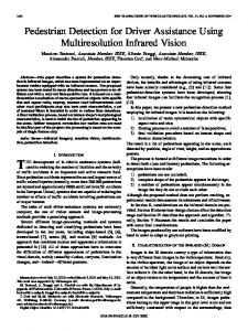
of the vulnerable road users (VRU), and more particularly pedestrians, still constitutes a critical and challenging problem due to the inherent complexity of the problem [1]; moreover, it is an appealing topic of research due to its direct impact in the society, been a promising tool for a lowering in traffic injuries. It is clear the strong correlation between the scientific progress achieved in the last years on pedestrian detection and the availability of public datasets. In this context, we made available a public dataset composed by laser scans and synchronized image frames. Laser labeled segments and the corresponding cut-outs (cropped images) are also accessible1 . A multilayer LIDAR, an Ibeo-Alasca XT, and a monocular camera, an Allied Guppy, constitute the sensor setup used to collect the dataset; the sensors apparatus was mounted in a rigid platform on the frontal part of an electrical vehicle, shown in Fig. 1, which was driven manually with a maximum speed of 30 Km/h.

Fig. 1. Electric vehicle and the sensor setup used for the dataset acquisition.

Succinctly, our detection system has four main modules: preprocessing and segmentation; feature extraction; tracking and data association; and classification. Feature selection,   coordinate transformation (calibration), classifier selection, information fusion, and context information are other important sub-modules of the detection system. The classification module, more specifically the proposed cascade framework, is the focus of this paper. Nevertheless, a brief discussion about preprocessing and segmentation is presented in section III, and a succinct description of the feature sets are described in sections III-A and III-B. Tracking and data association were introduced in a previous work [8]. In the remainder of this work the acronym LIDAR will be treated as a synonym of ‘laserscanner’ or simply ‘laser’. 1 http://www.isr.uc.pt/~cpremebida/dataset

II. LASER AND IMAGE DATASET Once our specific interest lies in comparing the classification performance of single classifiers and the proposed cascade method on pedestrian detection, using laser and image-based features, the following criteria were adopted to compose our dataset: •

•

•

• •

a positive sample is defined by a entire body pedestrian, in an upright position, present in both the camera and laser field of view (FOV). A negative sample is defined by any other object (non-pedestrian) present in the FOV of both sensors; the entities/objects of interest should be characterized, unambiguously, by a laser-segment and by its projected region of interest (ROI) in the image plane; the dataset is divided in two parts: a training set Dtrain , used to train the classifier parameters and also to perform cross-validation, bagging and feature selection; and the testing set Dtest used to evaluate the classification performance; both Dtrain and Dtest are partitioned in two subsets: laser Dlaser and image Dvision subsets; the dataset has cardinality defined by the number of samples and dimensionality defined by the number of features; it is not a raw dataset2 .

The elements of the dataset are feature vectors i.e., the sets and subsets are defined in terms of vector elements. More exactly, Dlaser = {fl1 , fl2 · · · fln : n = (ntrain + ntest ) is the total number of samples}, where flk is the kth laser-based feature vector. Similar definition is valid for Dvision (substituting fl by the image-based vectors fv ). The cardinality depends on the number of samples, e.g. |Dtrain | = ntrain , and the dimensionality varies with the number of features: |fl |, or |fv |, or the union of both. For clarity, the following notationSshould be observed laser vision in the Ssequel: Dtrain = Dtrain Dtrain , Dtest = S laser laser vision laser laser Dtest SDtest , D = Dtrain Dtest and Dvision = vision vision Dtrain Dtest . The manual labeling process, inherent to any supervised dataset, was carried out using laser segments (1) as primary reference for pedestrian and non-pedestrians annotation. The labeled segments, extracted from raw data scans, are validated using the corresponding image frame (for ground truth confirmation). All the segments of interest were labeled under user supervision, avoiding some problems invariably presented on realistic situations, such as: data association errors, over-segmentation, measurement missing, tracking inconsistencies, etc. However, it is important to mention that the image-based subset (cut-outs) were extracted directly, using calibration parameters, from the laser-segment projections in the image plane without user intervention or any post-processing; it means that all the cropped images, used to extract the image-features fv to compose Dvision , are in fact the ROI obtained directly from the labeled laser segments and, as consequence, are prone to error due to calibration 2 raw

laser data and images frames are also available.

imprecision, road irregularities, vehicle vibrations, and so on. Nevertheless, we decided to allow those cropped images with no user intervention or any correction, resulting in a closer realistic image-based dataset. The dataset, summarized in Table I, was acquired in the ISR-UC Campus 3 , under the following configuration: 1) Laser-based subset: the Ibeo LIDAR was mounted approximately 52 cm above the ground, with FOV restricted to 150o , horizontal angular resolution of 0.5o , and vertical resolution of [−1.6o , −0.8o , 0.8o , 1.6o ]; 2) Image-based subset: the camera was mounted above the laser, see Fig. 1, with FOV of ≈ 67o ; the intrinsic and extrinsic parameters are described in [9]. The positives correspond to pedestrians in static or moving states, and the negatives consist of posts, tree-trunks, hydrants, light-posts, walls, fences, bushes, foliage, cars, etc. The dataset and the corresponding ground truth, generated under user supervision, are available on the Web. TABLE I DATA SET: SUCCINCT STATISTICS Name

Total

Dtrain

1100

Dtest

1400

Training dataset Nneg. Description Sunny day, winter, collected 550 550 between 15:30 to 16:30 Testing dataset Sunny day, winter, collected 400 1000 between 12:00 to 17:30

Npos.

Dtrain and Dtest were collected on different dates. Although both sets were acquired around the same area, some samples of the testing part were acquired at dusk, where the illumination conditions changed drastically. Some images of the dataset are shown in Fig. 2. III. DATA PREPROCESSING AND FEATURE EXTRACTION The preprocessing module is composed by a set of processes, namely: pre-filtering, coordinate transformation, and segmentation. At this processing stage each entity (object) constitutes a hypothesis of being a positive (pedestrian) or a negative (non-pedestrian). Pre-filtering is composed by a set of pertinent data processing tasks necessary to decrease the complexity and the processing time of subsequent stages. Coordinate transformation is a conversion, accomplished in the laser space, from polar to the Cartesian coordinates. The segmentation stage constitutes a critical part in such perception systems, and can be performed by means of specific methods as presented in [10]. The segmentation process is performed in the LIDAR space, where the detected objects are characterized by a group/cluster of laser-points, here named segment. Expressing a 2D full scan as a sequence of ns measurement points in the form Scan = {(rl , αl )|l = 1, ..., ns}, where (rl , αl ) denotes the polar coordinates of the lth scan 3 http://www.isr.uc.pt/~cpremebida/PoloII-Google-map.pdf

Positives (testing)

ROI k

ROI k+1

Positives (training)

Sk+1 Sk Negatives (testing)

Laser­feature vectors

Fig. 3. An example with two positives (pedestrians) detected in the laser scan, characterized by Sk , Sk+1 , and the corresponding ROIs in the image plane (ROIk ,ROIk+1 ). The feature vectors are denoted by flk,k+1 and fvk,k+1 .

Negatives (training)

 

Fig. 2. Some samples to illustrate the different conditions and situations in which the dataset has been acquired.

point, a group of scan points that constitute a segment Sk can be expressed as Sk = {(rn , αn )}, n ∈ [li , lf ], n = 1, . . . , np

Image­feature vectors

(1)

where np is the number of points in the current segment, li and lf are the initial and the final scan points that define the segment. A segment can also be defined in Cartesian coordinates x = (xk , yk ), where (xk = rn cos αn , yk = rn sin αn ). Due to annotation purpose, mentioned in previous section, a segment is explicitly defined by a group of range-points related to one, unambiguously, object of interest. Although in realistic situations it does not occur in a deterministic way. In the next subsections we present the laser and imagebased features. The former feature set is a 18-dimensional vector (flk is calculated using the range-points (1)), and the vision feature set (a 256-dimensional vector fv ), is extracted from the ROI projections of the laser segments in the image plane. An example that illustrates two pedestrians perceived by the laser, as segments of range points Sk and Sk+1 , and its ROI in the image plane are depicted in Fig. 3. A. LIDAR-based features Features extracted from LIDAR data and its utilization for pedestrian detection and scenario interpretation are subjects addressed in [4], [7] and [11]. In previous works, we have used a 15-dimensional laser-based feature vector [9], most of them based on Arras’s work [11]. Now we extend this vector with three more attributes: • Standard Deviational Ellipse: r σx2 + σy2 (2) 2

 

where σx2 and σy2 are the variances in x and y Cartesian directions, respectively. While the standard distance deviation is a useful single measure of the dispersion around the mean center, it does not show the potential skewed nature of the points (anisotropy). The standard deviation ellipse gives dispersion in the two dimensions (x and y). • Unbiased distance deviation: np 2 X (Deucn ) np − 2 n=1

(3)

where Deucn is the Euclidean distance between each point xn and the mean center µx . • Euclidean distance dispersion: Pnp

n=1

Pnp Deuc2n − [( n=1 Deucn )2 ]/np np − 1

(4)

it is a measure of dispersion between the summation of the squared points and the square of the normalized summation. These additional features increased the classification performance, see section VI, compared with our previous 15dimensional laser feature vector [9]. The feature selection analysis showed that these new features bring relevance to the system, although some are closely redundant with some components of the complete laser-feature vector fl . B. Vision-based features The descriptors used to detect pedestrians in the imagebased subset are the well-known histogram of oriented gradients (HOG) [12], with 81 components, and covariance matrices descriptors (COV) [13], [14], with 175 descriptors, totalizing a 256-dimensional feature vector. This imagebased feature vector was adopted after a set of experiments performed over the Daimler Pedestrian Classification Benchmark Dataset (2006) using a set of classifiers and fusion methods for pedestrian detection in cropped images [15].

C. Feature selection In this work, we have filtered out the most lineardependent features, i.e. with correlation coefficient greater or equal to 0.99, as a first step to select the most relevant set of features. To prevent redundancy, and to take advantage of the diversity among the features, an approach based on mutual information was also used for feature selection. We have adopted the method named mRMR (minimum-Redundancy Maximum-Relevancy) [16] which is based on information theory. It is important to note that this feature selection method is independent, in terms of information theory, of the type of classifier; this generalization capability is very beneficial in pattern recognition problems. In our case, a feature selection method is almost mandatory once we are using a Naive Bayes and a Gaussian Mixture Models (GMMC) component classifiers, among others. Those classifiers are prone to inconsistencies (e.g. singularities on the covariance matrix, or likelihoods tending to zero) as the number of features and/or the complexity of the dataset increase; moreover, the conditionally independent of the features is a strong prerequisite for these classification machines, specifically for the Naive model.

where yhlimit is a point belonging to the hyperplane. Considering yhproj as the projection of point yh on the separatinghyperplane (7) and d as the distance between the separatinghyperplane (7) and yh, yields:

IV. SINGLE CLASSIFIERS Five single classifiers, FLDA, Naive-Bayes, GMMC, SVM-RBF and a multilayer perceptron neural network (NN), have been used as decision functions to separate the feature space in two classes, i.e. pedestrians and non-pedestrians classes. The first four methods are succinctly described in [9] and the latter, the NN-MMGDX [17] classifier, is a back-propagation method based on the Maximal Margin (MM) principle which directly increases the margin of the NN output-layer hyperplane. The MMGDX jointly optimizes both NN layers in a single process, back-propagating the gradient of an MM-based objective function, through the output and hidden layers, in order to create a hidden-layer space that enables a higher margin for the output-layer hyperplane. The unconstrained optimization problem

(11)

min

W1 ,b1 ,W2

J

(5)

is applied on model yh = ϕ(W1 x + b1 ) yb = ϕ(W2 yh + b2 )

(6)

where yh is the output vector of the hidden layer, Wk (k = 1, 2) is the synaptic weights matrix of the layer k, bk is the bias vector of layer k, x is the input vector, ϕ(.) is the sigmoid function. The output layer of model (6) has bias b2 = 0, because after the training section the ROC curve information is taken into account to adjust the classifier threshold, which acts as bias. The proposed MM-based objective function aims to stretch out the margin to its limit. Notice that, the separatinghyperplane of model (6) is given by W2 yhlimit = 0

(7)

yh − yhproj = d

W2T kW2 k

(8)

Multiplying both sides of (8) by W2 yields: W2 yh − W2 yhproj = d

W2 W2T kW2 k

(9)

As yhproj belongs to hyperplane (7), substituting (7) and the second line of (6) in (9), yields: d=

yˆ kW2 k

(10)

As the sigmoid activation function bounds the hidden neuron output in the interval [0, √ 1], the norm of vector yh has its maximum value equal to n, where n is the number of W2 hidden neurons. Taking into account that the norm of kW 2k is one, we can deduce that √ √ W2 − n≤ yh ≤ n kW2 k

√ √ i.e. the distance d (10) is bounded in the interval [− n, n]. Therefore, as the target output yi (where i denotes the training example index) assumes the values -1 or 1, we propose the error function   √ yˆi ei = yi n − (12) kW2 k in order to force the NN to stretch out the value of di (in this work defined as the classification margin of example i) to its limit, creating a hidden output space where the distance between patterns of different classes is as larger as possible. The objective function J is p

J = kEk p

(13)

where k·k is the Lp-norm, E = [e1 , e2 , . . . , eN ] is the error vector, and ei is defined in (12). The main idea is to calculate the functional J focusing specially on the support vectors margins, inspired on the SVM soft-margin training algorithm. The Lp-norm is a trick to avoid the constrained optimization problem usual in the SVM-like approach. Notice that, larger errors ei are related to support vectors (i.e. the patterns with small distance d from the separating-hyperplane), therefore, if the Lp-norm is applied, the larger is p the larger is the contribution of the larger errors in the calculation of the objective function J. In fact, if the power p → ∞ only the pattern with smallest distance from the separate hyperplane will be considered in the calculation of the objective function J. Backpropagation is used to calculate the derivatives of the objective function (13), which are required to apply the gradient descent training algorithm. All the single component classifiers have been trained and tested considering the entire feature set Dtrain and its

laser vision subsets Dtrain and Dtrain . The classifiers parameters’ were adjusted based on K-fold cross validation, that it, the labeled training dataset is partitioned in k subsamples, where k1 subsamples are used as traditional training set and the other subsets are used as validation set. The cross validation process is repeated k times, with each of the k split dataset part used only one time as the validation dataset. The results obtained with k validation subsets were used to select the classifiers’ parameters.

V. CASCADE CLASSIFIER

Feature_2

The cascade method proposed here has a training strategy decomposed in two phases, bagging and boosting, applied separately in the subsets Dlaser and Dvision . A contribution of this paper is the proposed bagging, or bootstrap aggregation, where a subset (Dbagg ) of the Dtrain is selected, the bagging part, for reusing in the training process in order to improve the final classification by means of an ensemble of classifiers (the boosting process). In the bagging procedure, the adopted partitioning criteria is based on the response of a base classifier, which is ‘boosted’ by a second, more complex and usually non-linear classifier trained in the subset Dbagg . Basically, Dbagg contains all the samples (true positives TP, true negatives TN, false positives FP, and false negatives FN) within a margin defined in the first stage. Figure 4 illustrates this procedure with a hypothetical bi-dimensional example. Boundary  decision

Margin:

Dtrain and Dbagg respectively, and the final decision classification is achieved considering the joint decision of the classifier’s ensemble: the boosting part. Actually, the process described above is performed in both feature spaces Dlaser and Dvision ; it means that the training method proposed here is carried out in two phases (Algorithm 1 is performed twice for each feature set): one using the laser features and the other with image-based features. Algorithm 1 Training process of the cascade ensemble. Input: {Dtrain }: training dataset ns : number of selected samples Classifiers: f c1 (first-stage); f c2 (second-stage) 1: {Dbagg } ← empty set 2: train f c1 using Dtrain to obtain the decision boundary 3: the margin L1 is obtained with a stopping criteria when: FP=0 and FN=0 and ns > T hr 4: {Dbagg } ← {Dtrain |ns }; 5: train f c2 using Dbagg Output: set of trained model {f c1 , f c2 }. Figure 5 illustrates the proposed cascade ensemble. This classifier composition can be used jointly, in both stages, or in a separate way. Considering the laser-stage, the final classification decision is defined jointly by f c1 and f c2 , laser laser trained with Dtrain and Dbagg respectively, where all the samples, within the decision margin of the first classifier, are inputs for the second classifier f c2 . The same functional principle is valid for the vision-stage, and also when both laser and image features are used. laser­stage

Laser features

Samples within the margin: 

feature_1

Fig. 4. Illustrative example of the bagging process: Dbagg is obtained considering the samples inside the margin defined by a linear classifier.

The proposed strategy for combining the cascade of classifiers has the following steps: 1) two single classifiers are considered in the training process: a base classifier (trained in Dtrain ), and a more robust classifier (trained in Dbagg ); 2) the subset Dbagg is formed re-sampling Dtrain with ns samples (positives and negatives) within the margin Li ; 3) Li is obtained starting from the decision frontier and stopping if the number of FP and FN is zero and ns > T hr, where T hr is at least 10% of the total number of samples; 4) the subset (Dbagg ⊂ Dtrain ) is used as training dataset for the second classifier; 5) the proposed cascade is formed with the above two classifiers, whose parameters were learned using

Positives and  Negatives

vision­stage

Image features

Positives and  Negatives

laser­stage

vision­stage

Laser­Image features

Positives and  Negatives

Fig. 5. Functional diagram of the cascade of classifiers regarding the sensor/feature to be used.

VI. RESULTS Experimental results were evaluated and compared in terms of accuracy (Acc), area under ROC curve (AUC), and balanced error rate (BER). These performance metrics are calculated over all samples presented on the testing set Dtest , hence those scores serve as a global indicator of the classifiers performance. To support specific analysis, we have selected a metric based on an useful percentile of the false positive rate, up to 10%, named T P r10% .

TABLE II P ERFORMANCE RESULTS FOR SINGLE - CLASSIFIERS SCHEME

A. Summary of the classifiers The FLDA and the Naive-Bayes are base classifiers, not requiring parameter adjustments. Eventually, for the case of Naive-Bayes classifiers, the likelihood tends to zero depending on the feature distributions. Based on k-fold cross validation performed during the training phase, the number of Gaussian components of the GMMC classifier was set to 5, and the margin parameter used in the SVM-RBF was 100. Moreover, the NN trained by MMGDX was configured with 5 neurons in the hidden layers. The cascade scheme was setup with FLDA and SVM-RBF in the first and second stages respectively. B. Classification performance

FLDA 0.903 0.834 0.121 0.575

AU C Acc BER T P r10%

FLDA 0.936 0.896 0.112 0.877

AU C Acc BER T P r10%

FLDA 0.937 0.891 0.116 0.850

TABLE III P ERFORMANCE RESULTS FOR THE C ASCADE CLASSIFIER laser {Dtest } 0.928 0.874 0.148 0.865

AU C Acc BER T P r10%

vision {Dtest } 0.916 0.856 0.153 0.733

1

0.9

FLDA Naive GMMC SVM-RBF NN-MMGDX

0.8

0.7

0.6

0.5

0.4

1

0.9

FLDA Naive GMMC SVM-RBF NN-MMGDX

0.2

0.1

0.1

0.1

0.2

0.3

0.4

0.5

0.6

False positives rate

0.7

0.8

0.9

0 0

1

(a) ROC: single classifiers scheme.

0.2

0.3

0.4

0.5

0.6

False positives rate

0.7

0.8

0.9

1

(b) ROC: cascade scheme.

Fig. 7. ROC curves for single-component and cascade classifiers over vision . vision dataset Dtest 1

0.9

FLDA Naive GMMC SVM-RBF NN-MMGDX

Cascade/Laser 0.7

Cascade/Complete

0.8

0.7

0.5

0.4

0.6

0.5

True positives rate

True positives rate

0.7

0.6

0.6

0.5

0.4

0.6

0.5

0.4

0.3

0.3

0.2

0.2

0.4

0.3

0.3

0.1

0.1

0.2

0.2

0 0

0.1

0.1

0 0

0.1

0.8

True positives rate

True positives rate

0.7

0.4

0.3

0.8

0.8

0.5

0.2

1

1

0.6

0.3

0.9

0.9

Cascade/Vision

0.8

True positives rate

0.7

0 0

{Dtest } 0.941 0.906 0.072 0.965

1

0.9

True positives rate

laser vision Performance results over Dtest , Dtest and Dtest datasets are summarized in Table II, where the best results are highlighted in bold format, and by ROC curves of Figs. 6(a), 7(a), and 8(a) respectively. The single classifier NNlaser MMGDX showed the most important results in the Dtest subset. Regarding the vision part of the testing set, the SVM with RBF kernel achieved the best performance. The results for the complete set (Dtest ) is favorable to NN-MMGDX which obtained better results than the other methods, however the SVM-RBF showed a close performance behavior in some metrics. The GMMC and the Naive classifiers were trained with 25% of the most relevant and less redundant features, see section III-C, to avoid inconsistencies (e.g., singularities on the covariance matrix, or likelihood tending to zero). The cascade scheme performance is summarized in Table III, and corresponding ROC curves are shown in Figs. 6(b), 7(b), and 8(b). Many configurations were experimented, during the k-cross validation stage, for deciding which arrangement to be used during the test analysis. Although multiple variations of the cascade scheme has been trained (changing the classifier method and/or the feature space), some of them with perfect separation within the training dataset, the final selected cascade structure did not achieve the expected results over the testing datasets.

AU C Acc BER T P r10%

laser } LIDAR subset:{Dtest Naive GMMC SVM-RBF NN-MMGDX 0.936 0.882 0.940 0.945 0.874 0.879 0.874 0.886 0.105 0.119 0.096 0.101 0.892 0.887 0.860 0.877 vision } Vision subset:{Dtest Naive GMMC SVM-RBF NN-MMGDX 0.838 0.884 0.976 0.963 0.801 0.886 0.929 0.852 0.226 0.136 0.087 0.110 0.320 0.893 0.953 0.922 Joint-features subset:{Dtest } Naive GMMC SVM-RBF NN-MMGDX 0.895 0.912 0.976 0.972 0.843 0.911 0.929 0.936 0.135 0.092 0.084 0.062 0.552 0.936 0.950 0.975

0.1

0.2

0.3

0.4

0.5

0.6

False positives rate

0.7

0.8

0.9

1

(a) ROC: single classifiers scheme.

0 0

0.1

0.2

0.3

0.4

0.5

0.6

False positives rate

0.7

0.8

0.9

1

(b) ROC: cascade scheme.

Fig. 6. ROC curves for single-component and cascade classifiers over laser laser . dataset Dtest

0.1

0.2

0.3

0.4

0.5

0.6

False positives rate

0.7

0.8

0.9

1

(a) ROC: single classifiers scheme.

0 0

0.1

0.2

0.3

0.4

0.5

0.6

False positives rate

0.7

0.8

0.9

1

(b) ROC: cascade scheme.

Fig. 8. ROC curves for single-component and cascade classifiers over the complete dataset Dtest .

VII. CONCLUSION AND FUTURE WORK A cascade classifier composed by the combination of two single classifiers, applied in pedestrian detection using laser and vision features, has been proposed and analyzed in this paper. Its classification performance has been characterized and comparisons with a set of single classifiers were presented. We are working to improve the cascade method, investigating different ways on combining the stages, in particular the number of features per subset and the component classifiers arrangement. This kind of boosting method, performed with expert classifiers (trained using distinct samples and feature subsets), is expected to lead to interesting results over datasets with strong unbalanced data, that is particularly true for urban scenarios. To pursuit a deep understanding on this topic, the collection and annotation of a more representative dataset, comprising thousands of images and laser’scans of negatives and pedestrians (some of them partially occluded), is on the way. Moreover, vehicle ego-motion information will be also available, based on the estimation of a stochastic filter that fuses measurements from a Real-Time Kinematic GPS, rotary encoders, and an inertial measurement unit. VIII. ACKNOWLEDGMENT The authors would like to thank Hugo Faria for his helpful assistance in programming and setting up part of the experimental platform. R EFERENCES [1] T. Gandhi and M.M. Trivedi. Pedestrian protection systems: issues, survey, and challenges. Intelligent Transportation Systems, IEEE Transactions on, 8(3):413–430, 2007. [2] M. Enzweiler and D. M. Gavrila. Monocular pedestrian detection: Survey and experiments. IEEE Transactions on Pattern Analysis and Machine Intelligence, 31(12):2179–2195, Oct. 2009. [3] P. Dollar, C. Wojek, B. Schiele, and P. Perona. Pedestrian detection: A benchmark. Computer Vision and Pattern Recognition, 2009. CVPR 2009. IEEE Conference on, pages 304–311, 20-25 2009. [4] D. Streller and K. Dietmayer. Object tracking and classification using a multiple hypothesis approach. In Intelligent Vehicles Symposium, IVS. IEEE, pages 808–812, June 2004. [5] S. Gidel, P. Checchin, C. Blanc, T. Chateau, and L. Trassoudaine. Pedestrian detection method using a multilayer laserscanner: Application in urban environment. Intelligent Robots and Systems, IROS. IEEE/RSJ International Conference on, pages 173–178, Sept. 2008. [6] L. Spinello and R. Siegwart. Human detection using multimodal and multidimensional features. In Robotics and Automation, ICRA. IEEE International Conference on, pages 3264–3269, May 2008. [7] B. Douillard, D. Fox, and F. Ramos. A spatio-temporal probabilistic model for multi-sensor object recognition. In Intelligent Robots and Systems, IROS. IEEE/RSJ International Conference on, pages 2402– 2408, 29 2007-Nov. 2 2007. [8] C. Premebida and U. Nunes. A multi-target tracking and gmmclassifier for intelligent vehicles. In Intelligent Transportation Systems, ITSC. IEEE International Conference on, pages 313–318, Sept. 2006. [9] C. Premebida, O. Ludwig, and U. Nunes. Lidar and vision-based pedestrian detection system. Journal of Field Robotics, Wiley Periodicals, Inc., 26(9):696–711, 2009. [10] C. Premebida and U. Nunes. Segmentation and geometric primitives extraction from 2d laser range data for mobile robot applications. In Proc. 5th National Robotics Festival (ROBOTICA), Coimbra, Portugal, 2005.

[11] K.O. Arras, O.M. Mozos, and W. Burgard. Using boosted features for the detection of people in 2d range data. In Robotics and Automation, IROS. IEEE International Conference on, pages 3402–3407, April 2007. [12] N. Dalal and B. Triggs. Histograms of oriented gradients for human detection. In Computer Vision and Pattern Recognition, CVPR. IEEE Conference on, pages 886–893, 2005. [13] O. Tuzel, F. Porikli, and P. Meer. Region covariance: A fast descriptor for detection and classification. In In Proc. 9th European Conf. on Computer Vision, pages 589–600, 2006. [14] O. Tuzel, F. Porikli, and P. Meer. Human detection via classification on riemannian manifolds. In Computer Vision and Pattern Recognition, CVPR. IEEE Conference on, pages 1–8, June 2007. [15] O. Ludwig, D. Delgado, V. Gonc¸alves, and U. Nunes. Trainable classifier-fusion schemes: an application to pedestrian detection. In Intelligent Transportation Systems, ITSC. IEEE International Conference on, 2009. [16] H. Peng, F. Long, and C. Ding. Feature selection based on mutual information criteria of max-dependency, max-relevance, and minredundancy. Pattern Analysis and Machine Intelligence, IEEE Transactions on, 27(8):1226–1238, Aug. 2005. [17] O. Ludwig and U. Nunes. Novel maximum-margin training algorithms for supervised neural networks. Neural Networks, IEEE Transactions on, 21(6):972–984, June 2010.