A Case Study of Using a Multilayered ... - Semantic Scholar

2828

IEEE TRANSACTIONS ON GEOSCIENCE AND REMOTE SENSING, VOL. 49, NO. 8, AUGUST 2011

A Case Study of Using a Multilayered Thermodynamical Snow Model for Radiance Assimilation Ally M. Toure, Kalifa Goïta, Alain Royer, Edward J. Kim, Michael Durand, Steven A. Margulis, and Huizhong Lu

Abstract—A microwave radiance assimilation (RA) scheme for the retrieval of snow physical state variables requires a snowpack physical model (SM) coupled to a radiative transfer model. In order to assimilate microwave brightness temperatures (Tbs) at horizontal polarization (h-pol), an SM capable of resolving melt–refreeze crusts is required. To date, it has not been shown whether an RA scheme is tractable with the large number of state variables present in such an SM or whether melt-refreeze crust densities can be estimated. In this paper, an RA scheme is presented using the CROCUS SM which is capable of resolving melt-refreeze crusts. We assimilated both vertical (v) and horizontal (h) Tbs at 18.7 and 36.5 GHz. We found that assimilating Tb at both h-pol and vertical polarization (v-pol) into CROCUS dramatically improved snow depth estimates, with a bias of 1.4 cm compared to −7.3 cm reported by previous studies. Assimilation of both h-pol and v-pol led to more accurate results than assimilation of v-pol alone. The snow water equivalent (SWE) bias of the RA scheme was 0.4 cm, while the bias of the SWE estimated by an empirical retrieval algorithm was −2.9 cm. Characterization of melt-refreeze crusts via an RA scheme is demonstrated here for the first time; the RA scheme correctly identified the location of melt-refreeze crusts observed in situ. Index Terms—Assimilation, melt–refreeze crusts, radiance, snow, snowpack model (SM).

I. I NTRODUCTION

S

EASONAL snow cover has a strong impact on climate, hydrological processes, and on human activities [1]. Snow is the frozen storage term in the water balance and is also a valuable resource. Monitoring snow physical variables

Manuscript received June 14, 2010; revised November 3, 2010 and January 22, 2011; accepted January 30, 2011. Date of publication April 29, 2011; date of current version July 22, 2011. This work was supported in part by the National Science and Engineering Research Council of Canada, by Environment Canada (Cryosphere System in Canada Program), and by the National Aeronautics and Space Administration Terrestrial Hydrology Program. A. M. Toure and E. J. Kim are with the National Aeronautics and Space Administration Goddard Space Flight Center, Global Modeling and Assimilation Office Code 610.1, Greenbelt, MD 20771 USA (e-mail: [email protected]; [email protected]). K. Goïta, A. Royer, and H. Lu are with Université de Sherbrooke, Sherbrooke, QC J1K 2R1, Canada (e-mail: [email protected]; [email protected]; [email protected]). M. Durand is with the School of Earth Sciences, The Ohio State University, Columbus, OH 43210 USA (e-mail: [email protected]). S. A. Margulis is with the Department of Civil and Environmental Engineering, University of California, Los Angeles, CA 90095 USA (e-mail: [email protected]). Color versions of one or more of the figures in this paper are available online at http://ieeexplore.ieee.org. Digital Object Identifier 10.1109/TGRS.2011.2118761

(extent, water equivalent, and melting conditions) is essential for weather and hydrological forecasts in many regions and provides information for meteorological forecasts, hydroelectric power generation, fresh water supply, river traffic, irrigation, runoff, and flood control [2]. Passive microwave-based estimates of terrestrial snow variables such as snow water equivalent (SWE) from satellite observations have so far been generated primarily by regression-based empirical methods. Snow variables retrieved by such methods are sometimes used in product-based data assimilation [3]–[5]. With this type of approach, the retrieval and the forward data assimilation do not necessarily have consistent physics or assumptions. Consistency is much easier to achieve when radiances are directly assimilated. This radiance assimilation (RA) approach has been used for years to retrieve atmospheric parameters by the operational weather forecasting community with great success [6]. This approach may also be an effective way to retrieve snow physical parameters such as snow depth and its water equivalent [7]. Snow RA requires accurate predictions of the brightness temperature (Tb) emitted by the snowpack. This imposes requirements on the key elements of the snow RA scheme: a snowpack model (SM), a radiative transfer model (RTM), and a data assimilation framework. In a previous study, Durand et al. [8] demonstrated that the microwave emission model for layered snowpacks (MEMLS) [9] has the ability to accurately predict the radiance when the snow layering structure and other state variables, such as grain-size correlation length, density, snow depth, liquid water, and temperature, are accurately represented. They also showed that the accuracy of RTMs particularly at horizontal polarization (h-pol) is highly sensitive to the stratigraphic representation of the snowpack and particularly to dense snow layers, such as melt–refreeze crusts. Durand et al. [10] subsequently demonstrated the potential of snow RA using the simple snow-atmosphere-soil transfer model (SAST) [11] SM coupled to MEMLS. SAST is a simple three-layer energy-balance scheme. An improvement of the simulation of snow depth was achieved through the use of an ensemble Kalman smoother scheme at this local scale for a weeklong study [10]. However, limitations of SAST (three layers and no representation of melt-refreeze crusts) were evident. Indeed, only Tbs at vertical polarization (v-pol) could be assimilated due to the fact that SAST does not adequately represent the vertical stratigraphy of the snowpack. This is inherently suboptimal, as only half of the available information could be assimilated; the h-pol channels were ignored. Assimilation of

0196-2892/$26.00 © 2011 IEEE

TOURE et al.: CASE STUDY OF USING A MULTILAYERED THERMODYNAMICAL SNOW MODEL

the h-pol channels thus requires an SM with higher vertical resolution. This is due to the fact that vertical variations in snow density lead to increased h-pol reflection coefficients at the layer interfaces within the snowpack; a melt-refreeze crust with a thickness of 1 cm can lead to a dramatic decrease in h-pol brightness [8]. While increasing the number of layers increases the fidelity of the RTM, it makes the assimilation problem much more difficult, however, as it increases the number of SM parameters that must be estimated using the assimilation scheme. In this follow-on study, we explore RA using a much more sophisticated snow model, i.e., the CROCUS snowpack model [12], [13]. CROCUS has been used for operational avalanche forecasting in France since 1992. It simulates the physical snowpack processes and layering (stratigraphy) using up to 50 layers; CROCUS tracks layers that undergo melt-refreeze metamorphism. In the RA scheme proposed in this paper, we treat precipitation, grain-size evolution, and the density evolution of melt-refreeze crusts as uncertain within the context of the assimilation framework, and we estimate snow depth as well as grain size and density for each layer in the CROCUS model (i.e., on the order of 100 state variables at each model time step). We seek to answer the following two questions: 1) When on the order of 100 state variables are estimated simultaneously, will there be adequate information in the observations to accurately characterize snow depth? Previous snow RA studies have estimated less than ten state variables per model time step, e.g., [10]. To date, it has not been shown whether a snow RA scheme is tractable with on the order of 100 state variables per time step; and 2) Do the measurements contain enough information to simultaneously estimate the vertical structure of the snowpack grain size and melt-refreeze crusts, as well as the snow depth? In this paper, we follow the convention in [14] and refer to snow layers resulting from partial melting and refreezing processes as “melt-refreeze crusts.” Note that melt-refreeze crusts so defined generally have densities lower than that of solid pure ice (ρice = 917 kg · m−3 ). In contrast to melt-refreeze crusts, pure ice has a glasslike appearance and is generally more homogeneous as melting has eliminated individual snow grains. Melt-refreeze crusts generally still consist of snow grains; some of which may have begun to adhere via melting/refreezing. We believe that this distinction may prove to be important for proper radiative transfer modeling; using an SM with more sophisticated representation of snow stratigraphy and meltrefreeze crusts should improve the accuracy of the prediction of the RA estimates. II. M ATERIAL AND M ETHODS A. Experimental Data Set Three types of in situ data were used in this paper: meteorological data to drive the SM, Tb data for assimilation within the RA scheme, and snowpit measurements for the validation of the RA estimates. We used meteorological, snowpit, and microwave radiance measurements collected during the National Aeronautics and Space Administration Cold Land Processes Field Experiment-1 (CLPX-1) [15], [16] in Colorado, USA.

2829

The CLPX-1 was a multisensor multiscale field campaign to provide a comprehensive data set for understanding fluxes, storage, and transformations of water and energy in cold land areas at regional and global scales. Intensive ground, airborne, and spaceborne observations were collected on a set of nested study areas, ranging from 1 ha to 160 000 km2 , selected to cover a wide range of physiographic conditions and spatial scales (www.nohrsc.nws.gov/~cline/clpx.html). Our study area is the local scale observation site (LSOS). LSOS was a 1-ha study site located within the 1-km2 -CLPX-1 Fraser intensive study area, near the Fraser experimental forest headquarters facility (39◦ 50# 49## N, 105◦ 54# 40## W, 2780 m above sea level). Our period was the intensive observation period-3 (IOP3) on February 19–25, 2003. IOP3 was characterized by dry snow except on February 25 [8]. The snowpit data on February 25 revealed the presence of wet snow. The presence of liquid water in the layer generally leads to melt/refreeze metamorphism [17] which can result in the formation of large irregular clusters of rounded crystals held together by large ice-to-ice bonds (larger grains grow at the expense of smaller ones). Liquid water retained in snow pores can refreeze during the following cool night (under clear sky), and partial melting may occur subsequently. Consecutive melt/refreeze cycles lead to the formation of meltrefreeze crusts [2] and ultimately to layers of true ice. 1) Snowpit Data: There were seven days (February 19–25, 2003) on which both snowpit data and Tb were collected at the LSOS. Snowpit data included the snow depth, SWE, snow density, snow temperature, snow stratigraphy, and snow grain size. The average snow depth and SWE during the IOP3 were 92.7 and 197 mm, respectively [15]. The snowpit data were collected from two different snowpit locations within 10 m of the radiometer footprint: pit #1 (on February 20, 22, and 24) and pit #2 (on February 19, 21, 23, and 25). On February 19, the data were collected at 12:10 local time (LT); on February 20 at 15:30 LT; on February 21 at 11:30 LT; on February 22 at 11:00 LT; on February 23 at 11:00 LT; on February 24 at 13:30 LT; and on February 25 at 11:00 LT. Snow temperature was measured at 10-cm vertical intervals. All snow layers were dry during IOP3 except on February 25 when wet snow was observed near the snow–air interface (surface temperature was between −0.2 ◦ C and +0.5 ◦ C). IOP3 snow-soil interface temperatures ranged from −0.2 ◦ C to −0.5 ◦ C [15]. Snow density was measured at 10-cm vertical intervals. The presence and location of melt-refreeze crusts was also identified and recorded, but melt-refreeze crust density was not measured in the field. Melt-refreeze crust density is generally lower than that of the pure ice (917 kg · m−3 ), depending on the amount of pore space in the layer [18]. The details of the location of melt-refreeze crusts observed in IOP3 are presented in [8, Fig. 4]. Some of the melt-refreeze crusts are due to meltrefreeze metamorphism that has occurred earlier in the season, outside of our experiment period. Snowfall events on February 20, 22, and 25 increased snow depth by approximately 20 cm as the total. Grain size was characterized by measuring the greatest spatial extension of the prevailing grains Dmax using a microscope with 8 × 30 optics [14]. Newly fallen snow with grain sizes

2830

IEEE TRANSACTIONS ON GEOSCIENCE AND REMOTE SENSING, VOL. 49, NO. 8, AUGUST 2011

ranging from 0.1 to 1.5 mm was observed in the upper part of the snowpack. Depth hoar was observed at the bottom of the snowpack with Dmax between 1.5 and 2.4 mm (see [8, Fig. 4]). Between these boundaries, mixed grain shapes were observed with Dmax ranging between 0.7 and 1 mm. During IOP3, the presence of melt-refreeze crusts was noticed in each snowpit except on February 22. The locations of the melt-refreeze crusts are different for each snowpit (see [8, Fig. 4]). This can be attributed to the local spatial variability of the site because each snowpit was excavated in a slightly different location. Fierz et al. [14] have defined snow grain size as the largest dimension (maximum diameter, Dmax ) of predominant snow grains. Dmax was measured in the field during the CLPX-1. Volume scattering of electromagnetic waves by a granular medium such as snow, however, does not depend upon Dmax [19], [20]. Physically meaningful structural parameters include the optical grain size (D0 ), the snow specific area (SSA), and the correlation length (Pex ) [20]–[24]. We used the empirical formula developed in [8] to estimate the Pex from the CLPX-1 Dmax measurements. 2) Meteorological Data: The meteorological station used was located near the ground-based microwave radiometer (GBMR-7) instrument from the University of Tokyo [16]. The meteorological data were collected between October 1, 2002 and March 29, 2003 with a 10-min temporal resolution. The data collected include wind speed, wind direction, air temperature, relative humidity, downward long-wave radiation, downward shortwave radiation, and precipitation. Three other meteorological forcing parameters needed to run the CROCUS (i.e., the cloud cover, the type of precipitation, and the diffuse solar radiation) were not measured in the field but were estimated as a function of measured meteorological (downward long-wave radiation, air temperature, and relative humidity) data using the Simplified Simple Biosphere (SSiB) land surface model [25]. 3) Radiometric Data: We used radiance observations from the GBMR-7 at 18.7 and 36.5 GHz at v- and h-pol from February 19 to February 25, 2003 (IOP3). The Tb observations were obtained between 12:30 and 15:30 LT on a daily basis [16]. Tbs were available for seven measurement times. We had four channels for a total number of 28 observations. The GBMR-7 was designed to withstand extreme outdoor conditions (−30 ◦ C/ + 40 ◦ C) [26]. The radiometer receiver electronics was encapsulated in a thermally stabilized container to ensure accurate measurements. The radiometers were calibrated before each scan using a combination of the cold/hot and Dicke switching techniques. An additional internal calibration was performed before each scan [16]. A mechanical positioner was used to vary the measurement incidence and azimuth angles. Two different snow measurement techniques were used: 1) azimuth scans of undisturbed total snow cover with varying azimuth (140◦ –210◦ ) with a fixed incidence angle of 55◦ ; and 2) angular scans with varying incidence angles (30◦ –70◦ ) with fixed azimuth angle of 180 [16]. In this paper, we use the azimuth because the location of the footprint was closer to the IOP3 snowpits (in situ observation used to validate the RA) for a majority of the azimuth scans (see [8], Fig. 3). These observations were also the closest in time to the snowpit observations performed

on the same day. Variations of several kelvins were observed within each azimuth scan [8]. Details of the viewing geometry of the instrument including the incidence angle and the azimuth can be found in [16] and in [8]. B. Models and the EnKF 1) Snow Physical Model: CROCUS is a 1-D multilayer SM designed to simulate the evolution of the vertical profile of the physical properties of the snowpack under given meteorological conditions [12], [13]. In contrast with simple SMs used in previous studies, CROCUS simulates up to 50 layers for snowpacks. CROCUS has a variable internal temporal resolution for evaluating mass and energy exchanges between the snowpack and the low-level atmosphere as functions of meteorological conditions [27]. The optimum time step is 15 min [13]. A smaller internal time step (for example, 5 min) yields more accurate results but requires more computation. Furthermore, a smaller internal time step leads to the formation of thin snow layers since the total precipitation for the time step decreases for the smaller time step. The meteorological forcing parameters include air temperature, wind speed, humidity, the amount and type of precipitation (rain or snow), direct downwelling shortwave radiation, downwelling long-wave radiation, diffuse solar radiation, and cloudiness. CROCUS output parameters include the type and size of grains for each snowpack layer along with layer thickness, temperature, density, and liquid water content. Additionally, the model tracks a variable indicating whether liquid water or faceted crystals have been predicted [13]. In short, CROCUS has significantly greater physical fidelity compared to the SAST three-layer model used in the previous snow RA study. Snow grain metamorphism is described in CROCUS by the shape parameters, namely, dendricity and sphericity. Dendricity varies from one to zero and describes how much of the original precipitated crystal form is still present in the snow layer. Sphericity ranges from zero for completely faceted grain to one for rounded particles [13]. MEMLS and CROCUS do not have the same way of representing the grain size. MEMLS uses the correlation length [20], and CROCUS uses the dendricity and sphericity. Details of the relationship between the dendricity and sphericity with the snow D0 can be seen in [13]. The D0 is defined as the diameter of a sphere with the same total surface area and the same volume as the real distribution of snow grains in a given layer [19]. The SSA of a granular medium is the ratio of the surface area of the grains divided by their total volume [20]. According to [20] and [28], the relation between the Pex , the SSA, and the D0 (calculated by CROCUS) is as follows: Pex = 4

2 (1 − fice ) = (1 − fice )D0 SSA 3

(1)

where fice = ρ/ρice is the volume fraction of the ice, ρ is the density of the snow, and ρice = 917 kg · m−3 is the density of pure ice. 2) RTM: The MEMLS [9], [29] was developed for the frequency range from 5 to 100 GHz. It is based on an RTM which

TOURE et al.: CASE STUDY OF USING A MULTILAYERED THERMODYNAMICAL SNOW MODEL

takes multiple volume scattering and absorption into account. In this paper, the scattering coefficient is derived from snowslab experiments with dry winter snow [9] and using the improved Born approximation theory, [30] and the absorption coefficient, refraction, reflection at layer interfaces, and the effective permittivity are based on physical models and on measured ice and snow dielectric properties. MEMLS has been validated for both fine-grained snow [9] and for melt-refreeze crusts [30]. Because MEMLS has the ability to handle snow as a multilayered medium as well as calculate extinction coefficients for melt-refreeze crusts, it is ideal for this study. MEMLS requires the following inputs: thickness, density, temperature, liquid water content, and correlation length for each snow layer. MEMLS uses the correlation length Pex to compute the scattering coefficient. 3) EnKF: The SM is used to develop a priori estimates of the snowpack states or the state forecast vector y fi for replicate (an individual model realization using one unique set of perturbations) i at time t. This is expressed mathematically by y fi,t = F (y i,0 , u i,t , β i )

(2)

where F () is the SM operator (CROCUS in our case; the forecasting model), y i,0 is the state initial condition, u i,t is the meteorological forcing data for replicate i, and β i represents the unknown parameters controlling grain size and meltrefreeze crust evolution (described in the following section). Note that vectors and matrices are marked by boldface characters and the scalars by ordinary italics. The a posteriori state estimate or analysis vector y ai is computed as a linear combination of the a priori estimate y fi and a weighted difference between the actual measurement z obs and the measurement prediction M(y fi ) as (time subscripts are omitted) ! " #$ (3) y ai = y fi + K (z obs − µi ) − M y fi

where µi is the random measurement error that prevents the introduction of correlations among the replicates [31] and K is the Kalman gain calculated from the error covariances provided by the ensemble (see [7]). C. Experimental Setup Our RA scheme consists of three components: 1) A snow physical model (CROCUS) prognoses snowpack structure and is driven by meteorological data; 2) An RTM (MEMLS) simulates Tb using the predicted snowpack state variables predicted by CROCUS; and 3) The Ensemble Kalman Filter (EnKF) updates the predicted snowpack state variables. While the data and EnKF framework are consistent with previous work [10], the CROCUS SM used in this paper resolves the snowpack in far greater detail. The more sophisticated SM used herein fundamentally changes the estimation problem because of the following: 1) The horizontal Tb was not assimilated in [10], since the SM used in that study was not capable of resolving melt-refreeze crusts and therefore not capable of simulating horizontal Tb; and (2) the number of snowpack state variables

2831

for the three-layered SM used in previous work is far less than the number of state variables simulated by CROCUS, which increases the complexity of the estimation problem. Using the models described earlier, we performed an RA experiment. In order to have a benchmark by which the performance of the RA can be evaluated, CROCUS was run using the measured precipitation data and without assimilating GBMR-7 measurements. These results are referred to as the “open-loop” run hereafter. An “open-loop” simulation is defined as a forward model run without implementing/enacting the RA procedure [7]. In this paper, the “open-loop” run was a single model run performed using the nominal model inputs. The ensemble was constructed by perturbing the CROCUS inputs as follows: We assumed that, for modeling snow physics during the accumulation season, the three dominant sources of uncertainty in the SM run are: 1) the precipitation measurements; 2) the grain-size parameterization (grain-size physics models are still under development [7]); and 3) the modeling of the melt-refreeze crusts. These three sources of uncertainty are taken into account in the RA by treating key variables in the model inputs as random variables. The measured precipitation forcing data were perturbed with a multiplicative timecorrelated lognormal forcing error with an assumed coefficient of variation of 0.25, based on the value used in previous work [10]. The coefficients of growth of the grain-size parameters (see [13]) were randomly perturbed. The coefficient of variation is assumed to be 0.5 for the grain-size growth parameter. We also treated the parameter controlling density evolution for melt-refreeze crusts as an uncertain random variable and applied a multiplicative lognormal random perturbation. Fifty combinations of perturbed random input variables were used in the RA. For each ensemble member realization of meteorological data and model parameters, CROCUS was run to obtain an a priori estimate. The a posteriori estimate was obtained by assimilating GBMR-7 Tb using the EnKF technique. In this paper, we performed two assimilation experiments. First, we followed previous studies and assimilated only Tb at v-pol (TbV). Second, we experimented with assimilating both TbV and Tb at h-pol (TbH). Based on [8], we know that TbH is very sensitive to melt-refreeze crusts. By modeling melt-refreeze crusts and treating them as random variables, we allow for the possibility of using the TbH channels, effectively doubling the number of measurements that can be assimilated. Doing this is only possible with a physical SM such as CROCUS that has enough vertical resolution (up to 50 layers) and snow physics to model melt-refreeze crusts, particularly the melt-refreeze crusts noted at LSOS snowpits [15]. III. R ESULTS AND D ISCUSSION In this section, we present the results of the two RA experiments described earlier. In the first experiment, only TbV is assimilated; in the second experiment, both TbV and TbH are assimilated. RA estimates of snow depth, SWE, snow grain size, and snow density are compared with in situ measurements and with the open-loop model run. Additionally, the RA snow depth estimates are compared with the results obtained in [10] in previous work. Finally, the RA SWE estimates are compared

2832

IEEE TRANSACTIONS ON GEOSCIENCE AND REMOTE SENSING, VOL. 49, NO. 8, AUGUST 2011

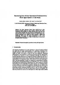
Fig. 1. Retrieved (a) snow depth and (b) SWE by assimilating GBMR-7 TbV and TbH for an ensemble size of 50 replicates. TABLE I DAILY E RROR AND RMSE OF THE S NOW D EPTH E STIMATE ( IN C ENTIMETER ) BASED ON A SSIMILATION I NTO CROCUS OF T B M EASURED BY THE GBMR-7 (E RROR _V R EPRESENTS THE E RRORS IN THE C ASE OF T B V A SSIMILATION AND E RROR _H_V R EPRESENTS THE C ASE OF B OTH T B H AND T B V A SSIMILATION ) C OMPARED TO E RRORS FOR THE O PEN -L OOP RUN AND E RRORS O BTAINED BY D URAND ET AL. [10] (E RROR _SAST) BY A SSIMILATING GBMR-7 I NTO SAST M ODEL . VALUES IN PARENTHESIS R EPRESENT THE R ATIO ( IN P ERCENT ) OF THE RMSE D IVIDED BY THE AVERAGE IOP3 S NOW D EPTH

with empirical algorithm SWE estimates derived directly from the observations. In all of the comparisons hereinafter, the mean across the a posteriori ensemble is used to represent the RA-derived estimate of the snow state variables. A. Snow Depth Comparisons As expected, the open-loop model run underestimates the measured snow depth significantly [7], [10] (Fig. 1). The openloop bias is 28.2 cm, and the root mean square error (RMSE) is 28.5 cm. This large bias of the open-loop case was also noticed in [10], using the SAST land surface model and is attributed primarily to the precipitation undercatch at the meteorological station. The open-loop model runs form one baseline against which to evaluate the EnKF. While a calibrated model might perform better, we would argue that, in general, snow precipitation undercatch remains a significant problem; our goal is to determine whether the RA scheme can correct both for these precipitation errors and for the grain size and melt-refreeze crust prediction errors. In the first RA experiment, only the TbV measurements were assimilated using the EnKF. The results of this experiment are shown in Table I. The estimate of snow depth is improved as

compared with the open loop, with a bias of −3.10 cm and an RMSE of 5.10 cm. The RMSE is thus reduced by 82.1%, and the absolute value of the bias is reduced by 89% as compared to the open loop. In the second experiment, both TbV and TbH were assimilated. The results of this experiment are shown in Fig. 1(a). The snow depth estimates in this case show additional improvement (see Table I). The bias is reduced to 1.4 cm and the RMSE to 4.5 cm, demonstrating an improvement of 54.8% and 11.8%, respectively, compared with assimilation of only TbV. These results indicate that significant improvement in snowpack estimates can be obtained by utilizing both the h- and v-pol channels. In order to utilize the TbH channels, however, the SM must have the capability to resolve meltrefreeze crusts. For both experiments, these results show significant improvement compared to the 7.3-cm bias found in [10] obtained by assimilating the GBMR-7 TbV into SAST. Since, here, we used the exact same forcing and the same RTM with the same EnKF assimilation technique, only the SM was different. Fig. 1(a) shows the posterior and open-loop snow depth calculated during IOP3. These results suggest that the use of the more sophisticated CROCUS model permits higher fidelity snowpack modeling leading to smaller bias in the characterization of snow depth.

TOURE et al.: CASE STUDY OF USING A MULTILAYERED THERMODYNAMICAL SNOW MODEL

2833

TABLE II DAILY E RROR AND RMSE OF THE SWE E STIMATE ( IN C ENTIMETER ) BASED ON A SSIMILATION OF T B V AND T B H (SWE R ETRIEVED ) C OMPARED TO E RRORS OF THE SWE O PEN L OOP AND SWE R ETRIEVAL U SING THE C HANG ET AL. [32] R ETRIEVAL F ORMULA . VALUES IN PARENTHESIS R EPRESENT THE R ATIO ( IN P ERCENT ) OF THE RMSE D IVIDED BY THE AVERAGE IOP3 SWE

Fig. 2. IOP3 in situ snow (a), (c), (e) optical grain size and (b), (c), (f) density vertical profiles compared to the open-loop simulation and RA from February 19, 2003 to February 21, 2003. The snow depth is normalized to one.

B. SWE Comparison Fig. 1(b) shows the estimated SWE compared to the openloop case and the in situ data. The open-loop underestimates the in situ SWE. The bias is 9.4 cm, and the RMSE is 9.5 cm. When the TbV and TbH were assimilated in CROCUS, the SWE estimate is improved, the bias is 0.44 cm, and the RMSE is 1.4 cm (see Table II). We compared the results of RA to that of the snapshot retrieval formula used in [32], referred to as the “Chang” retrieval hereafter. The bias of Chang SWE is −2.87 cm. The formula was originally derived to estimate snow depth using the difference of the TbH at 18 and 36 GHz scaled by a time static coefficient (based on homogeneous grain-size

radius of 0.3 mm and a constant density of 300 kg · m−3 ). The comparison shows that RA using CROCUS performs better than the empirical model because it is able to provide detailed and time-varying snow a priori information. C. Grain-Size Comparison Snow optical grain size was calculated using the equations established by Brun et al. [13]. These equations relate the optical grain size to the dendricity and the sphericity simulated by CROCUS. We plotted the optical grain-size profiles for the seven days of the IOP3. Figs. 2(a), (c), (e), 3(a), (c), (e), and 4(a) are the representations of the optical grain-size vertical profiles

2834

IEEE TRANSACTIONS ON GEOSCIENCE AND REMOTE SENSING, VOL. 49, NO. 8, AUGUST 2011

Fig. 3. IOP3 in situ snow (a), (c), (e) optical grain size and (b), (c), (f) density vertical profiles compared to the open-loop simulation and RA from February 22, 2003 to February 24, 2003. The snow depth is normalized to one.

Fig. 4. IOP3 in situ snow (a) optical grain size and (b) density vertical profiles compared to the open-loop simulation and RA on February 25, 2003. The snow depth is normalized to one.

for the seven days of the IOP3. The figures showed that there are systematic underestimates of grain size in the open loop when compared with the in situ, and that, those underestimates are corrected by the posterior. The grain size of the bottom layer (i.e., the snow layer that is in contact with the ground) was low for the first three days of the RA. For the last three days, the grain size increased dramatically to values ranging between 2 and 3.7 mm. Predicting grain growth during melt/refreeze meta-

morphism responsible for the formation of coarse snow grain size is a complex task, and the theories used by CROCUS are yet to be extensively validated. However, it is very significant that the assimilation scheme predicts large grain-size values in the bottom of the snowpack. For most of the snowpits, meltrefreeze crusts were observed near the bottom of the snowpack (see [8], Fig. 4). The values of the grain size predicted by the RA scheme in Figs. 2–4 are in the range measured in [33] for

TOURE et al.: CASE STUDY OF USING A MULTILAYERED THERMODYNAMICAL SNOW MODEL

2835

TABLE III DAILY E RROR AND RMSE OF T B ( IN K ELVIN ) S IMULATED BY CROCUS+MEMLS U SING THE A Posteriori S NOW C HARACTERISTICS C OMPARED TO GBMR-7 M EASUREMENTS

melt-refreeze crusts. The open-loop grain size lower in the pack is qualitatively too low to belong to melt-refreeze crusts. While the melt-refreeze crust grain size was not measured during IOP3, the aforementioned analysis gives qualitative support for the hypothesis that the RA scheme is adjusting grain size in a way that is consistent with what is known about snow during IOP3 and the grain size of melt-refreeze crusts. D. Density Comparison Figs. 2(b), (d), (f), 3(b), (d), (f), and 4(b) show the density vertical profiles for all the IOP3. The figures show that the openloop snow density profiles underestimate the snow density. The EnKF estimate is much closer to the in situ average density expected at the bottom of the profile and for normalized snow depths at around 0.4 and 0.6 for the first three days and for depth around 0.4 for the last four days. The CROCUS historical index of the bottom layer for the entire IOP3 is five which indicates that the layers underwent multiple wet metamorphisms (see earlier discussion for model details). Despite this, the open-loop density value is rather low, approximately 200 kg · m−3 . The reason for this may point to an issue with the melt-refreeze crust evolution in the CROCUS model. Within the RA scheme, however, the melt-refreeze crust prognostic scheme is treated as uncertain, which allows the EnKF to prescribe a large update to the melt-refreeze crust density. On the 19th and the 20th, the a posteriori density of the melt-refreeze crusts at the bottom of the pack is around 650 kg · m−3 . From the 21st to the 25th, the density increased to reach values between 850 kg · m−3 and 900 kg · m−3 . Because the density of the melt-refreeze crusts was not measured in situ, it is impossible to validate these estimates. However, there is no doubt from the in situ snowpit observations that melt-refreeze crusts were observed in the bottom of the snowpack. Moreover, literature values for the density of melt-refreeze crusts [33], [34] range from 440 to 950 kg · m−3 . Clearly, the melt-refreeze crust densities estimated by the RA scheme are in the range of those reported in the literature, while the open-loop densities are less than the literature values. To study the impact of the correction of melt-refreeze crust density by the RA on the simulated Tb, we used the posterior estimates of snow characteristic as input to MEMLS to simulate the Tb. Table III shows bias and RMSE between the modeled and the measured GBMR-7 Tb for each of the seven days and for each of the four measurement channels. The update of the melt-refreeze crust density leads to an accurate simulation

of the TbH. This is not surprising, of course, because the EnKF scheme is designed to minimize the differences between the observed and predicted Tbs. Nonetheless, this comparison is valuable because it provides an additional check that the CROCUS+MEMLS simulations have been made consistent with the GBMR-7 observations. In Durand et al. [10], only the TbV was used in the RA, and only the snow depth and grain size were retrieved. Here, we have used RA to adjust the melt-refreeze crust density for a better prediction of TbH. In doing so, we anticipate that assimilating the TbH in addition to the TbV can help retrieve the snow depth with at least the same accuracy as in [10] and also the SWE. Although we do not have ground truth data for the melt-refreeze crust density, we note that the depth and SWE estimates are improved when TbH is assimilated, and that, the melt-refreeze crust density and grain-size values from the RA scheme are consistent with the values reported in the literature, while the open-loop values of grain size and density of the meltrefreeze crusts are less than the literature values. Moreover, the RA scheme effectively increased melt-refreeze crust densities in a way that is completely consistent with the known location of melt-refreeze crusts from the snowpits. This is the first time that RA has been used to adjust the density of melt-refreeze crusts for a better retrieval of snow depth and SWE. The fact that RA using a more sophisticated SM is able to retrieve snow density and optical grain-size profiles illustrates a crucial point: There is adequate information in the microwave signal, if applied within the RA framework, to extract the vertical structure of the grain size and density profiles with greater fidelity than when using a three-layered SM, at least at the point scale. The many-to-one problem of the SWE–Tb relationship can be overcome by assimilation, even when the density and grain-size profiles vary significantly with depth. The ability of CROCUS to model melt-refreeze crusts is clearly imperfect. Indeed, when run outside the assimilation framework, CROCUS does not adequately model melt-refreeze crusts: The modeled densities are far less than those typical for melt-refreeze crusts. It is only when the densification is treated as a random process and the radiance measurements are utilized within the assimilation scheme that the melt-refreeze crust densities are identified. Thus, radiance assimilation schemes must incorporate uncertainty in the densification processes that lead to melt-refreeze crusts. If they are neglected, then only vpol channels should be utilized. If h-pol channels are utilized and uncertainty in the melt-refreeze crusts is neglected, then errors in SWE or depth can be quite significant.

2836

IEEE TRANSACTIONS ON GEOSCIENCE AND REMOTE SENSING, VOL. 49, NO. 8, AUGUST 2011

IV. C ONCLUSION Experiments have been performed to evaluate the accuracy of RA to estimate the snow physical parameters using a more realistic SM (CROCUS) versus earlier snow RA studies. Precipitation and CROCUS model parameters controlling grain-size growth and melt-refreeze crust density evolution were treated as uncertain. The RA scheme treated the snow depth, density, and grain size as the state variables and assimilated ground-based Tb at 18.7 and 36.5 GHz. We have compared results from assimilating only TbV and from assimilating both TbH and TbV. We have found that the RA scheme accurately characterized the snow depth and SWE, and that assimilation of both TbH and TbV improved the retrieval of the snow depth and SWE compared with assimilating only one polarization. The a posteriori bias from the RA scheme was reduced to 1.4 cm and the RMSE to 4.5 cm compared with an open-loop bias and RMSE of 28.2 and 28.5 cm, respectively. The snow depth bias obtained here is significantly less than that reported in a previous RA study [10], suggesting that the use of the more sophisticated CROCUS model permits higher fidelity snowpack modeling leading to smaller bias in the characterization of snow depth. We have hypothesized that the improvement in snow depth and SWE over previous studies is due in part to the use of the TbH channels, which is made possible by the CROCUS and RA characterization of melt-refreeze crust densities. The RA scheme correctly identified the location of melt-refreeze crusts observed in situ. Moreover, the melt-refreeze crust densities estimated by the RA scheme are in the range of those reported in the literature, while the open-loop densities are less than the literature values. These improvements suggest that using a more sophisticated model such as CROCUS, RA is also able to update melt-refreeze crust density, which may lead to an improvement of the estimation of snow depth and SWE under more complex snow conditions than previously considered. ACKNOWLEDGMENT The authors would like to thank C. Mätzler for the use of microwave emission model for layered snowpacks, the Centre d’Étude de la Neige, France, for providing us with CROCUS, and all of the Cold Land Processes Field Experiment participants for collecting the data used in this study. Computational resources were provided by the Réseau Québécois de Calcul de Haute Performance and Compute Canada. R EFERENCES [1] R. L. Armstrong and E. Brun, Snow and Climate: Physical Processes, Surface Energy Exchange and Modeling. Cambridge, U.K.: Cambridge Univ. Press, 2008, 256p. [2] C. Mätzler, “Applications of the interaction of microwaves with the natural snow cover,” Remote Sens. Rev., vol. 2, no. 2, pp. 259–387, 1987. [3] C. J. Sun, J. P. Walker, and R. Houser, “A methodology for snow data assimilation in a land surface model,” J. Geophys. Res., vol. 109, p. D08108, 2004, DOI: 10.1029/2003JD003765. [4] J. Pulliainen, “Mapping of snow water equivalent and snow depth in boreal and sub-arctic zones by assimilating space-borne microwave radiometer data and ground-based observations,” Remote Sens. Environ., vol. 101, no. 2, pp. 257–269, Mar. 2006. [5] J. Dong, J. P. Walker, P. R. Houser, and C. Sun, “Scanning multichannel microwave radiometer snow water equivalent assimilation,” J. Geophys. Res., vol. 112, p. D07108, 2007, DOI: 10.1029/2006JD007209.

[6] P. L. Houtekamer and H. L. Mitchell, “Data assimilation using an ensemble Kalman filter technique,” Mon. Wea. Rev., vol. 126, no. 3, pp. 796–811, Mar. 1998. [7] M. Durand and S. Margulis, “Feasibility test of multi-frequency radiometric data assimilation to estimate snow water equivalent,” J. Hydrometeor., vol. 7, no. 3, pp. 443–457, Jun. 2006. [8] M. Durand, E. J. Kim, and S. A. Margulis, “Quantifying uncertainty in modeling snow microwave radiance at the point-scale, including stratigraphic effects,” IEEE Trans. Geosci. Remote Sens., vol. 46, no. 6, pp. 1753–1767, Jun. 2008. [9] A. Wiesmann and C. Mätzler, “Microwave emission model of layered snowpacks,” Remote Sens. Environ., vol. 70, no. 3, pp. 307–316, Dec. 1999. [10] M. Durand, E. J. Kim, and S. A. Margulis, “Radiance assimilation shows promise for snowpack characterization,” Geophys. Res. Lett., vol. 36, p. L02503, 2009, DOI: 10.1029/2008GL035214. [11] S. F. Sun, J. M. Jin, and Y. Xue, “A simple snow-atmosphere-soil transfer model,” J. Geophys. Res., vol. 104, no. D16, pp. 19 587–19 597, 1999. [12] E. Brun, E. Martin, V. Simon, C. Gendre, and C. Coleou, “An energy and mass model of snow cover suitable for operational avalanche forecasting,” J. Glaciol., vol. 35, pp. 333–342, 1989. [13] E. Brun, P. David, M. Sudul, and G. Brunot, “A numerical model to simulate snow-cover stratigraphy,” J. Glaciol., vol. 38, pp. 13–22, 1992. [14] C. Fierz, R. L. Armstrong, Y. Durand, P. Etchevers, E. Greene, D. M. McClung, K. Nishimura, P. K. Satyawali, and S. A. Sokratov, “The international classification for seasonal snow on the ground,” IHPVII Technical Documents in Hydrology No 83, IACS Contribution No 1, UNESCO-IHP, Paris, France, 2009. [15] D. Cline, R. Armstrong, R. Davis, K. Elder, and G. Liston, “CLPX GBMR snow pit measurements,” in CLPX-Ground: Ground Based Passive Microwave Radiometer (GBMR-7) Data, M. Parsons and M. J. Brodzik, Eds. Boulder, CO: Nat. Snow Ice Data Center. Digital Media, 2003, Updated Jul. 2004. [16] T. Graf, T. Koike, H. Fujii, M. Brodzik, and R. Armstrong, CLPXGround: Ground Based Passive Microwave Radiometer (GBMR-7) Data. Boulder, CO: Nat. Snow Ice Data Center. Digital Media, 2003. [17] R. L. Armstrong, “Metamorphism in a subfreezing, seasonal snowcover: The role of thermal and vapor pressure conditions,” Ph.D. dissertation, Dept. Geography, Univ. Colorado, Boulder, CO, 1985, 175 pp. [18] A. Wiesmann, C. Mätzler, and T. Wiese, “Radiometric and structural measurements of snow samples,” Radio Sci., vol. 33, no. 2, pp. 273–289, 1998. [19] T. C. Grenfell and S. G. Warren, “Representation of a nonspherical ice particle by a collection of independent spheres for scattering and absorption of radiation,” J. Geophys. Res., vol. 104, pp. 31 697–31 709, 1999. [20] C. Mätzler, “Relation between grain size and correlation length of snow,” J. Glaciol., vol. 48, no. 162, pp. 461–466, Jun. 2002. [21] A. Stogryn, “Correlation functions for random granular media in strong fluctuation theory,” IEEE Trans. Geosci. Remote Sens., vol. GRS-22, no. 2, pp. 150–154, Mar. 1984. [22] H. Lim, M. E. Veysoglu, S. H. Yueh, R. T. Shin, and J. A. Kong, “Random medium model approach to scattering from a random collection of discrete scatters,” J. Electromagn. Waves Appl., vol. 8, no. 7, pp. 801–817, Jul. 1994. [23] C. Mätzler, “Autocorrelation function of granular media with free arrangement of spheres, spherical shells or ellipsoids,” J. Appl. Phys., vol. 81, no. 3, pp. 1509–1517, Feb. 1997. [24] A. M. Toure, K. Goïta, A. Royer, C. Mätzler, and M. Schneebeli, “Nearinfrared digital photography to estimate snow correlation length for microwave emission modeling,” Appl. Opt., vol. 47, no. 36, pp. 6723–6733, Dec. 2008. [25] Y. Xue, P. Sellers, J. L. Kinter, and J. Shukla, “A simplified biosphere model for global climate studies,” J. Clim., vol. 4, no. 3, pp. 345–364, Mar. 1991. [26] S. Kazama, T. Rose, and R. Zimmerman, “A precision autocalibrating 7 channel radiometer for environmental research applications,” J. Remote Sens. Soc. Jpn., vol. 19, no. 3, pp. 37–45, 1999. [27] Y. Lejeune, P. Wagnon, L. Bouilloud, P. Chevallier, P. Etchevers, E. Martin, E. Sicart, and F. Habets, “Melting of snow cover in a tropical mountain environment in Bolivia: Processes and modelling,” J. Hydrometeor., vol. 8, no. 4, pp. 922–937, Aug. 2007. [28] P. Debye, H. R. Anderson, and H. Brumberger, “Scattering by an inhomogeneous solid II. The Correlation function and its applications,” J. Appl. Phys., vol. 28, no. 6, pp. 679–683, Jun. 1957. [29] C. Mätzler and A. Wiesmann, “Extension of the microwave emission model of layered snowpacks to coarse-grained snow,” Remote Sens. Environ., vol. 70, no. 3, pp. 317–325, Dec. 1999.

TOURE et al.: CASE STUDY OF USING A MULTILAYERED THERMODYNAMICAL SNOW MODEL

[30] C. Mätzler, “Improved Born approximation for scattering of radiation in a granular medium,” J. Appl. Phys., vol. 83, no. 11, pp. 6111–6117, Jun. 1998. [31] G. Burgers, P. J. van Leeuwen, and G. Evensen, “Analysis scheme in the ensemble Kalman filter,” Mon. Wea. Rev., vol. 126, no. 6, pp. 1719–1724, Jun. 1998. [32] A. T. C. Chang, J. L. Foster, and D. K. Hall, “Nimbus-7 SMMR derived global snow cover parameters,” Ann. Glaciol., vol. 9, pp. 39–44, 1987. [33] P. Marsh and M. K. Woo, “Wetting front advance and freezing of meltwater within a snow cover 1. Observations in the Canadian arctic,” Water Resour. Res., vol. 20, no. 12, pp. 1853–1864, Dec. 1984. [34] W. T. Pfeffer and N. F. Humphrey. (1997). Determination of timing and location of water movement and ice-layer formation by temperature measurements in sub-freezing snow. J. Glaciol. [Online]. 43, pp. 292–304. Available: www.nohrsc.nws.gov/~cline/clpx.html

Ally M. Toure received the B.S. degree in environmental engineering from the University Hassan II, Casablanca, Morocco, in 1998, the M.S. degree in geological engineering from the School of Engineering Mohammedia, Rabat, Morocco, in 2001, and the Ph.D. degree in microwave remote sensing from the University of Sherbrooke, Sherbrooke, QC, Canada, in 2009. He is currently a Research Associate with the Goddard Earth Sciences and Technology Center, University of Maryland, Baltimore County, as a member of the Research Faculty and working on snow data assimilation at the Global Modeling and Assimilation Office, National Aeronautics and Space Administration Goddard Space Flight Center. His main research interests include land surface remote sensing, snow microwave emission modeling, and data assimilation.

Kalifa Goïta received the B.E. degree in surveying engineering from the École Nationale d’Ingénieurs, Bamako, Mali, in 1987, and the M.Sc. and Ph.D. degrees in remote sensing from the Université de Sherbrooke, Sherbrooke, QC, Canada, in 1991 and 1995, respectively. He was a Postdoctoral Fellow at the Climate Research Branch, Environment Canada, Toronto, ON, Canada, from 1995 to 1997. From 1997 to 2002, he was with the Faculty of Forestry, Université de Moncton, NB, Canada, as a Professor of remote sensing and geographic information system. Since June 2002, he has been a Professor of geomatics with the Université de Sherbrooke, where he has also been a Research Scientist with the Centre d’applications et de recherche en Télédétection. He has been the Head of the Department of Applied Geomatics, Université de Sherbrooke, since January 2009. His expertise includes both physical aspects of remote sensing (retrieval of biophysical parameters from visible to microwave spectrum) and GIS applications to environmental modeling. Dr. Goïta was the recipient of the Canadian Remote Sensing Society Award for the best Ph.D. thesis in remote sensing in 1995.

Alain Royer received the Ph.D. degree in geophysics from the University of Grenoble, Grenoble, France, in 1981. From 1983 to 1988, he was a Natural Sciences and Engineering Research Council Fellow with the Centre d’Applications et de Recherches en Télédétection (CARTEL), Université de Sherbrooke, Sherbrooke, QC, Canada. In 1988, he became a member of the professorial team of the Université de Sherbrooke. Between 2000 and 2010, he was the Head of CARTEL. His research interests are environmental geophysics from space, including the development of surface parameter retrieval algorithms from remote sensing data applied to northern climate change analysis. He was involved in the International Polar Year Canadian Cryosphere Project from 2008 to 2011, in collaboration with Environment Canada, for improving remote sensing of snow using passive microwave radiometry.

2837

Edward J. Kim received the S.B. and S.M. degrees in electrical engineering from the Massachusetts Institute of Technology, Cambridge, and completed the joint Ph.D. degree with the Department of Electrical Engineering and the Department of Atmospheric Sciences from the University of Michigan, Ann Arbor, in 1998. Since 1999, he has been with National Aeronautics and Space Administration Goddard Space Flight Center, Greenbelt, MD, developing and applying techniques primarily for cryospheric and water cycle remote sensing. He is the principal contact at Goddard in support of snow satellite concepts and has been a Member of several teams for operational snow retrieval algorithms. He serves as an Instrument Scientist for the Advanced Technology Microwave Sounder on the National Polar-orbiting Operational Environmental Satellite System Preparatory Project and Joint Polar Satellite System satellites and is also a Member of the European Space Agency’s Validation and Retrieval Team for the Soil Moisture and Ocean Salinity soil moisture mission. His research interests include the modeling of snow, ice, soil, and vegetation; radiative transfer theory; radiance assimilation; and the development of new observational tools. Dr. Kim was selected, in 1997, for a National Research Council Research Associateship, and in 1998, he was the recipient of Second Prize in the International Geoscience and Remote Sensing Symposium student paper competition. He is an Associate Editor for the IEEE G EOSCIENCE AND R EMOTE S ENSING L ETTERS.

Michael Durand received the B.S. degree in mechanical engineering and biological systems engineering from Virginia Polytechnic Institute, Blacksburg, in 2002, and the M.S. and Ph.D. degrees in civil engineering from the University of California, Los Angeles, in 2004 and 2007, respectively. He is currently an Assistant Professor with the School of Earth Sciences, The Ohio State University, Columbus.

Steven A. Margulis received the B.S. degree in civil and environmental engineering from the University of Southern California, Los Angeles, in 1996, and studied hydrology at the Massachusetts Institute of Technology, Cambridge, where he received the M.S. and Ph.D. degrees in civil and environmental engineering, in 1998 and 2002, respectively. He is currently an Associate Professor with the Department of Civil and Environmental Engineering, University of California, Los Angeles, where his research focus is on terrestrial hydrology, hydrometeorology, remote sensing, and data assimilation.

Huizhong Lu received the B.S. degree in mathematics from Wuhan University, Wuhan, China, in 1991, and the M.S. and Ph.D degrees in applied mathematics (numerical analysis) from the University of South Paris, Orsay, France, in 1992 and 1996, respectively. He was a Research Associate in numerical fluids mechanics with Laboratoire d’Informatique pour la Mécanique et les Sciences de l’Ingénieur, Centre National de la Recherche Scientifique, Orsay, France, from 1996 to 1999, and in theoretical chemistry with the University of Sherbrooke, Sherbrooke, QC, Canada, from 1999 to 2005. Since 2005, he has been a Scientific Computation Analyst with the Scientific Computer Center, Réseau québécois de calcul de haute performance, Sherbrooke. His research interests are developing, optimizing, and parallelizing numerical methods/algorithms from different disciplines—theoretical research in physics, acoustic/fluids mechanics, and medical and other image processing.