made explicitly in the theory of Petri nets, but sensible in a wider context, is that between .... These data give the category HL of Hoare languages. Observe that ...
In proceedings of CONCUR ’93, LNCS n. 715, 1993
A Classification of Models for Concurrency Vladimiro Sassone∗ Mogens Nielsen∗∗ Glynn Winskel ∗∗ ∗
∗∗
Dipartimento di Informatica, Universit`a di Pisa, Italy Computer Science Department, Aarhus University, Denmark
Extended Abstract Models for concurrency can be classified with respect to the three relevant parameters: behaviour/system, interleaving/noninterleaving, linear/branching time. When modelling a process, a choice concerning such parameters corresponds to choosing the level of abstraction of the resulting semantics. The classifications are formalised through the medium of category theory.
Introduction From its beginning, many efforts in the development of the theory of concurrency have been devoted to the study of suitable models for concurrent and distributed processes, and to the formal understanding of their semantics. As a result, in addition to standard models like languages, automata and transition systems [4, 9], models like Petri nets [8], process algebras [6, 2], Hoare traces [3], Mazurkiewicz traces [5], synchronization trees [15] and event structures [7, 16] have been introduced. The idea common to the models above is that they are based on atomic units of change—be they called transitions, actions, events or symbols from an alphabet—which are indivisible and constitute the steps out of which computations are built. The difference between the models may be expressed in terms of the parameters according to which models are often classified. For instance, a distinction made explicitly in the theory of Petri nets, but sensible in a wider context, is that between so-called “system” models allowing an explicit representation of the (possibly repeating) states in a system, and “behaviour” models abstracting away from such information, which focus instead on the behaviour in terms of patterns of occurrences of actions over time. Prime examples of the first type are transition systems and Petri nets, and of the second type, trees, event structures and traces. Thus, we can distinguish among models according to whether they ∗ This
author has been supported by a grant of the Danish Research Academy.
82
Beh./Int./Lin. Beh./Int./Bran. Beh./Nonint./Lin. Beh./Nonint./Bran. Sys./Int./Lin. Sys./Int./Bran. Sys./Nonint./Lin. Sys./Nonint./Bran.
Hoare languages synchronization trees deterministic labelled event structures labelled event structures deterministic transition systems transition systems deterministic transition systems with independence transition systems with independence
HL ST dLES LES dTS TS dTSI TSI
Table 1: The models are system models or behaviour models, in this sense; whether they can faithfully take into account the difference between concurrency and nondeterminism; and, finally, whether they can represent the branching structure of processes, i.e., the points in which choices are taken, or not. Relevant parameters when looking at models for concurrency are Behaviour or System model; Interleaving or Noninterleaving model; Linear or Branching Time model. The parameters cited correspond to choices in the level of abstraction at which we examine processes and which are not necessarily fixed for the process once and for all. It is the application one has in mind for the formal semantics which guides the choice of abstraction level. This work presents a classification of models for concurrency based on the three parameters, which represents a further step towards the identification of systematic connections between transition based models. In particular, we study a representative for each of the eight classes of models obtained by varying the parameters behaviour/system, interleaving/noninterleaving and linear/branching in all the possible ways. Intuitively, the situation can be graphically represented, as in the picture below, by a three-dimensional frame of reference whose coordinate axes represent the three parameters. ↑| | || || Lin/Bran ր || || || || Int/NonInt ←−−−−−−−−−−−| Beh/Sys ||
Our choices of models are summarized in Table 1. It is worth noticing that, with the exception of the new model of transition systems with independence, each model is well-known. The formal relationships between models are studied in a categorical setting, using the standard categorical tool of adjunctions. The “translations” between 83
models we shall consider are coreflections or reflections. These are particular kinds of adjunctions between two categories which imply that one category is embedded , fully and faithfully, in another.1 Here we draw on our experience in recasting models for concurrency as categories, detailed in [17]. Briefly the idea is that each model (transition systems are one such model) will be equipped with a notion of morphism, making it into a category in which the operations of process calculi are universal constructions. The morphisms will preserve behaviour, at the same time respecting a choice of granularity of the atomic changes in the description of processes—the morphisms are forms of simulations. One role of the morphisms is to relate the behaviour of a construction on processes to that of its components. The reflections and coreflections provide a way to express that one model is embedded in (is more abstract than) another, even when the two models are expressed in very different mathematical terms. One adjoint will say how to embed the more abstract model in the other, the other will abstract away from some aspect of the representation. The preservation properties of adjoints can be used to show how a semantics in one model translates to a semantics in another. The picture below, in which arrows represent coreflections and the “backward” arrows reflections, shows the “cube” of relationships. TSI ⊳−−−−−−−−−֓ TS △ .. △ .......... | || || || || || .. || . ..� � || || || −−֓ dTS dTSI ⊳−−−−−−− | ∪ ∪ △ △ | || || −−−−−−֓ ST LES ⊳−−− || || .. .. || .......... .......... || || || || | . . ∪ ∪ ..� ..� dLES ⊳−−−−−−−−−֓ HL .. .........
Although most of the chosen models are well known, among the adjunctions in the cube only HL ֒−⊳ ST, ST ֒−⊲ TS and ST ֒−⊲ LES have already appeared in literature. Here all proofs are omitted. The reader interested in the details is referred to [10, 11]. Some of the results presented here will appear in [17].
1
Interleaving Models
In this section, we study the interleaving models. We start by briefly recalling some well-known relationships between languages, trees and transition systems [17], and then, we study how they relate to deterministic transition systems. 1 Here a coreflection is an adjunction in which the unit is natural isomorphism, and a reflection an adjunction where the counit is a natural isomorphism.
84
Definition 1.1 (Labelled Transition Systems) A labelled transition system is a structure T = (S, sI , L, Tran) where S is a set of states; sI ∈ S is the initial state, L is a set of labels, and Tran ⊆ S × L × S is the transition relation. Given the labelled transition systems T0 and T1 , a morphism h: T0 → T1 is a pair (σ, λ), where σ: ST0 → ST1 is a function and λ: LT0 ⇀ LT1 a partial function, such that2 i) σ(sIT0 ) = sIT1 ; � � ii) (s, a, s′ ) ∈ Tran T0 implies if λ↓a then σ(s), λ(a), σ(s′ ) ∈ Tran T1 ; σ(s) = σ(s′ ) otherwise. This defines the category TS of labelled transition systems. Definition 1.2 (Synchronization Trees) A synchronization tree is an acyclic, reachable transition system S such that (s′ , a, s), (s′′ , b, s) ∈ Tran S
implies
s′ = s′′
and a = b.
We write ST to denote the full subcategory of TS consisting of synchronization trees. Definition 1.3 (Hoare Languages) A Hoare language is a pair (H, L), where ∅ 6= H ⊆ L∗ , and sa ∈ H ⇒ s ∈ H. A partial map λ: L0 ⇀ L1 is a morphism of Hoare languages from (H0 , L0 ) ˆ ˆ L∗ → L∗ is defined by to (H1 , L1 ) if for each s ∈ H0 it is λ(s) ∈ H1 , where λ: 0 1 � ˆ λ(s)λ(a) if λ↓a; ˆ ˆ λ(ǫ) =ǫ and λ(sa) = ˆ λ(s) otherwise. These data give the category HL of Hoare languages. Observe that any language (H, L) can be seen as a synchronization tree just by considering the strings of the language as states, the empty string being a the initial state, and defining a transition relation where s −→ s′ if and only if sa = s′ . This extends to a functor from HL to ST. This functor and the inclusion functor from ST to TS may be viewed as embeddings, as stated in the following theorem, where ֒−⊲ represents a coreflection and ֒−⊳ a reflection, and the functors from right to left abstract away from information about states (from TS to ST) and branching structure (from ST to HL). Theorem 1.4 HL ֒−−−−−−−⊳ ST ֒−−−−−−−⊲ TS 2 We
use f ↓x to mean that a partial function f is defined on argument x.
85
The right adjoint from TS to ST is the well-known construction of unfolding, while the left adjoint from ST to HL is a straightforward “set of paths” construction. The existence of a (co)reflection from category A to B tells us that there is a full subcategory of B which is equivalent (in the formal sense of equivalences of categories) to A. Therefore, once we have established a (co)reflection, it is sometimes interesting to identify such subcategories. In the case of HL and ST such a question is answered below. Proposition 1.5 (Languages are deterministic Trees) The full subcategory of ST consisting of those synchronization trees which are deterministic, say dST, is equivalent to the category of Hoare languages. Speaking informally, behaviour/system and linear/branching are independent parameters, and we expect to be able to forget the branching structure of a transition system without necessarily losing all the internal structure of the system. This leads us to identify a class of models able to represent the internal structure of processes without keeping track of their branching, i.e., the points at which the choices are actually taken. A suitable model is given by deterministic transition systems. Definition 1.6 (Deterministic Transition Systems) A transition system T is deterministic if (s, a, s′ ), (s, a, s′′ ) ∈ Tran T
implies
s′ = s′′ .
Let dTS be the full subcategory of TS consisting of those transition systems which are deterministic. Consider the binary relation ≃ on the state of a transition system T defined as the least equivalence which is forward closed, i.e., s ≃ s′
and (s, a, u), (s′ , a, u′ ) ∈ Tran T ⇒ u ≃ u′ ; � � and define ts.dts(T ) = S/≃, [sIT ]≃ , LT , Tran ≃ , where S/≃ are the equivalence classes of ≃, and � � s, a, s¯′ ) ∈ Tran T with s¯ ≃ s and s¯′ ≃ s′ . [s]≃ , a, [s′ ]≃ ∈ Tran ≃ ⇔ ∃(¯
This construction defines a functor which is left adjoint to the inclusion dTS ֒→ TS. Next, let us present a universal construction from Hoare languages to deterministic transition system. In particular, we exhibit a coreflection HL ֒−⊲ dTS. Let (H, L) be a language. The left adjoint is defined on objects as follows: hl .dts(H, L) = (H, ǫ, L, Tran), where (s, a, sa) ∈ Tran for any sa ∈ H, which is trivially a deterministic transition system. The right adjoint is a standard “set of traces” construction. Thus, we have enriched our diagram and we have a square. 86
Theorem 1.7 (The Interleaving Surface) dTS ֒−−−−−−−−−⊳ △ || || || || || ∪
TS △ || || || || || ∪
֒−−−−−−−−−⊳
ST
HL
Observe that the construction of the deterministic transition system associated to a language coincides exactly with the construction of the corresponding synchronization tree. However, due to the different objects in the categories, the type of universality of the construction changes. In other words, the same construction shows that HL is reflective in ST—a full subcategory of TS—and coreflective in dTS—another full subcategory of TS.
2
Non Interleaving vs. Interleaving Models
Event structures [7, 16] abstract away from the cyclic structure of the process and consider only events (strictly speaking event occurrences), assumed to be the atomic computational steps, and the cause/effect relationships between them. Thus, we can classify event structures as behavioural, branching and noninterleaving models. Here, we are interested in labelled event structures. Definition 2.1 (Labelled Event Structures) A labelled event structure is a structure ES = (E, #, ≤, ℓ, L) consisting of a set of events E partially ordered by ≤; a symmetric, irreflexive relation # ⊆ E × E, the conflict relation, such that { e′ ∈ E | e′ ≤ e } is finite for each e ∈ E, e # e′ ≤ e′′ implies e # e′′ for each e, e′ , e′′ ∈ E; a set of labels L and a labelling function ℓ: E → L. For an event e ∈ E, define ⌊e⌋ = { e′ ∈ E | e′ ≤ e }. Moreover, we write ∨∨ for # ∪ { (e, e) | e ∈ EES }. 2 These data define a relation of concurrency on events: co = EES \ (≤ ∪ ≤−1 ∪ #). A labelled event structure morphism from ES 0 to ES 1 is a pair of partial functions (η, λ), where η: EES 0 ⇀ EES 1 and λ: LES 0 ⇀ LES 1 are such that i) ⌊η(e)⌋ ⊆ η(⌊e⌋); ii) η(e) ∨∨ η(e′ ) implies e ∨∨ e′ ; iii) λ ◦ ℓES 0 = ℓES 1 ◦ η. This defines the category LES of labelled event structures. 87
The computational intuition behind event structures is simple: an event e can occur when all its causes, i.e., ⌊e⌋ \ {e}, have occurred and no event which is in conflict with has already occurred. This is formalized by the following notion of configuration. Definition 2.2 (Configurations) Given a labelled event structure ES , define the configurations of ES to be those subsets c ⊆ EES which are Conflict Free: ∀e1 , e2 ∈ c, not e1 # e2 Left Closed: ∀e ∈ c ∀e′ ≤ e, e′ ∈ c Let L(ES ) denote the set of configurations of ES . We say that e is enabled at a configuration c, in symbols c ⊢ e, if (i)
e 6∈ c;
(ii)
⌊e⌋ \ {e} ⊆ c;
(iii)
e′ ∈ EES and e′ # e implies e′ 6∈ c.
Although it is not the only possible one (see [11], where a category of pomset languages and a category of generalized trace languages are considered), a fair choice for behavioural, linear and noninterleaving models is given by deterministic labelled event structures. Definition 2.3 (Deterministic Labelled Event Structures) A labelled event structure ES is deterministic if for any c ∈ L(ES ), and for any pair of events e, e′ ∈ EES , whenever c ⊢ e, c ⊢ e′ and ℓ(e) = ℓ(e′ ), then e = e′ . This defines the category dLES as a full subcategory of LES. In [14], it is shown that synchronization trees and labelled event structures are related by a coreflection from ST to LES. The left adjoint associates with an ST-object S, a LES-object where the events are the transitions of S, ≤ is the tree-ordering of these, and # is the relation of incompatibility of transitions in this ordering. Hence co is empty, and in fact, the analogous of Proposition 1.5 for this coreflection states that synchronization trees are event structures with empty concurrency relations. The coreflection ST ֒−⊲ LES restricts to a coreflection dST ֒−⊲ dLES, and hence, by Proposition 1.5, to a coreflection HL ֒−⊲ dLES. Now, on the system level we look for a way of equipping transition systems with a notion of “concurrency” or “independence”, in the same way as LES may be seen as adding “concurrency” to ST. Moreover, such enriched transition systems should also represent the “system model” version of event structures. Several such models have appeared in the literature [12, 1, 13]. Here we choose a variation of these. Definition 2.4 (Transition Systems with Independence) A transition system with independence is a structure (S, sI , L, Tran, I) consisting of a transition system (S, sI , L, Tran) together with an irreflexive, symmetric relation I ⊆ Tran 2 such that 88
i) (s, a, s′ ) ∼ (s, a, s′′ ) ii) (s, a, s′ ) I (s, b, s′′ )
i.e.,
iii) (s, a, s′ ) I (s′ , b, u)
⇒
∃u. (s, a, s′ ) I (s′ , b, u) and (s, b, s′′ ) I (s′′ , a, u);
⇒
s
s′ = s′′ ;
s a � @ �b R @ ′
⇒
s′′
s a � @ �b � R @ ′ ′′ ⇒ s � � s @ b@ R a u
∃s′′. (s, a, s′ ) I (s, b, s′′ ) and (s, b, s′′ ) I (s′′ , a, u);
a i.e., s′ � @ b@ R
s
s a � @ �b � R @ ′ ′′ ⇒ s � � s @ b@ R a u
u
iv) (s, a, s′ ) ∼ (s′′ , a, u) I (w, b, w′ )
⇒
(s, a, s′ ) I (w, b, w′ );
where ∼ is least equivalence on transitions including the relation ≺ defined by s
′
′′
(s, a, s ) ≺ (s , a, u) ⇔
′
′′
(s, a, s ) I (s, b, s ) and (s, a, s′ ) I (s′ , b, u) and (s, b, s′′ ) I (s′′ , a, u).
H � Hb H j ′′ H a
s � ? ≺ s′ H a H ? H j b H u
Morphisms of transition systems with independence are morphisms of the underlying transition systems which preserve independence, i.e., such that � � � � (s, a, s′ ) I (¯ s, b, s¯′ ) and λ↓a, λ↓b ⇒ σ(s), λ(a), σ(s′ ) I σ(¯ s), λ(b), σ(¯ s′ ) . These data define the category TSI of transition systems with independence. Moreover, let dTSI denote the full subcategory of TSI consisting of transition systems with independence whose underlying transition system is deterministic. Thus, transition systems with independence are precisely standard transition systems but with an additional relation expressing when one transition is independent of another. The relation ∼, defined as the reflexive, symmetric and transitive closure of a relation ≺ which simply identifies local “diamonds” of concurrency, expresses when two transitions represent occurrences of the same event. Thus, the equivalence classes [(s, a, s′ )]∼ of transitions (s, a, s′ ) are the events of the transition system with independence. Transition systems with independence admit TS as a coreflective subcategory. In this case, the adjunction is easy. The left adjoint associates to any 89
transition system T the transition system with independence whose underlying transition system is T itself and whose independence relation is empty. The right adjoint simply forgets about the independence, mapping any transition system with independence to its underlying transition system. From the definition of morphisms of transition systems with independence, it follows easily that these mappings extend to functors which form a coreflection TS ֒−⊲ TSI. Moreover, such a coreflection trivially restricts to a coreflection dTS ֒−⊲ dTSI. So, we are led to the following diagram. Theorem 2.5 (Moving along the “interleaving/noninterleaving” axis) ⊳−−−−−−−−−֓ TS ... △ ......... | || || || . ..� || ⊳−−−−−−−−−֓ dTS | △ ∪ || LES ⊳−−− || −−−−−−֓ . ST || ......... || || ∪ ..�. ⊳−−−−−−−−−֓ HL TSI
dTSI
dLES
3
Non Interleaving Models
Now, the question is whether the relationships between the interleaving models generalize to our chosen noninterleaving counterparts. This is indeed so, and in the following we sketch the generalizations and their proofs. First of all, it is quite easy to see that the inclusion functor from ST to TS generalizes naturally to a functor les.tsi from LES to TSI. Consider a labelled event structure ES = (E, ≤, #, ℓ, L). Define les.tsi (ES ) to be the transition system with independence of the finite configurations of ES , i.e., � � les.tsi(ES ) = LF (ES ), ∅, L, Tran, I ,
where
• LF (ES ) is the set of finite configuration of ES ; • (c, a, c′ ) ∈ Tran if and only if c = c′ \ {e} and ℓ(e) = a; • (c, a, c′ ) I (¯ c, b, c¯′ ) if and only if (c′ \ c) co (¯ c′ \ c¯). This is basically nothing but formalizing the computational intuition of event structures (Definition 2.2) in terms of TSI. Our proof that this is part of a coreflection, involves (yet another) characterization of LES—here in terms of TSI—which also supports our claim of transition systems with independence being a “generalization” of event structures. 90
Theorem 3.1 (Event Structures are Transition Systems with Independence) Let oTSI (occurrence transition systems with independence) denote the full subcategory of TSI where the objects OTI = (S, sI , L, Tran, I) are reachable, acyclic and such that (s′ , a, u) 6= (s′′ , b, u) ∈ Tran implies ∃s. (s, b, s′ ) I (s, a, s′′ ) and (s, b, s′ ) I (s′ , a, u) and (s, a, s′′ ) I (s′′ , b, u),
(1)
or, in other words, (s′ , a, u) and (s′′ , b, u) form the bottom of a concurrency diamond, and t I t′
(2)
⇒
∃s. (s, a, s′ ) ∼ t
and (s, b, s′′ ) ∼ t′ .
Then oTSI and LES are equivalent categories. Moreover, the equivalence cuts down to an equivalence of doTSI and dLES. It is immediate to realize that les.tsi (ES ) is an occurrence transition system with independence; thus, les.tsi factorizes through les.otsi : LES → oTSI and the inclusion oTSI ֒→ TSI. In order to give a hint about the equivalences of Theorem 3.1, we sketch the transformation from oTSI to LES opposite to les.otsi. The labelled event structure associated to OTI is � � otsi.les(OTI ) = Tran OTI /∼, ≤, #, ℓ, LOTI ,
where
• [(s, a, s′ )]∼ ≤ [(¯ s, b, s¯′ )]∼
if and only if
for any path π of OTI , • [(s, a, s′ )]∼ # [(¯ s, b, s¯′ )]∼
[(¯ s, b, s¯′ )]∼ ∈ π
⇒
[(s, a, s′ )]∼ ∈ π;
⇒
[(s, a, s′ )]∼ 6∈ π;
if and only if
for any path π of OTI ,
[(¯ s, b, s¯′ )]∼ ∈ π
� � • ℓ [(s, a, s′ )]∼ = a;
and where we write [(s, a, s′ )]∼ ∈ π to mean that a representative of [(s, a, s′ )]∼ occurs in the path π. An example of this construction is given in Figure 1. The proof of Theorem 3.1 consists of showing that otsi.les and les.otsi form an equivalence of categories. Now, the right adjoint to les.tsi can be defined in terms of a notion of unfolding tsi.otsi of TSI’s into oTSI’s which is the right adjoint of the inclusion functor. The unfolding construction takes into account that computations which only differ for the order in which (representatives of) independent events (∼-classes) occur must be considered equivalent. Thus, differently from the interleaving 91
d�
•
6 c �
e b � •
•
≺ @ I a@ @
•
≺
•
≺
@ a I @ @
d
@ a I @ @ •
� d
e
� c
@ a I @ @
otsi.les
-
•
a
� b
#
c
@ @ @ @
•
b
•
Figure 1: case, the unfolding is not a tree: the states reached by equivalent computations coincide in the unfolded transition system. The proof that this form a coreflection is rather involved, but once established it is quite easy to see that it restricts to a coreflection doTSI ֒−⊲ dTSI. Thus, we have the coreflections LES ֒−⊲ TSI and dLES ֒−⊲ dTSI. The result is summarized in the following theorem. Theorem 3.2 (Moving along the “behaviour/system” axis)
dTSI △ || || || || || ∪ dLES
TSI ⊳−−−−−−−−−֓ TS △ ... △ ......... | || || || || || || . ..� || || || −−֓ dTS ⊳−−−−−−− | △ ∪ ∪ || LES ⊳−−− || −−−−−−֓ ST .. || ......... || || . ∪ ..� ⊳−−−−−−−−−֓ HL
Finally, we consider the relationship between dTSI and TSI, looking for a generalization of the reflection dTS ֒−⊳ TS. Of course, the question to be answered is whether a left adjoint for the inclusion functor dTSI ֒→ TSI exists or not. This is actually a complicated issue and for a long while we could not see the answer. However, we can now answer positively! The definition of the functor and the proof of the reflection are rather involved, since the presence of an independence relation, together with the axioms of transition systems with independence, raises considerably the complexity of the problem we faced easily 92
in the interleaving case. In particular, the object component of the functor is an inductive construction which builds on ts.dts taking independence into account. It is quite easy to realize that applying the quotient construction which defines ts.dts to transition systems with independence does not yield transition systems with independence, since it does not preserve the irreflexivity of the independence relation and properties (ii) and (iii) of Definition 2.4. However, an inductive construction which “completes” the outcome of ts.dts, building a transition system with independence upon it, can be defined. Technically, this is achieved by constructing an ω-chain of transition systems which fail to be transition systems with independence at most because of the irreflexivity of the independence relation and axioms (ii) and (iii), say pre-transition systems with independence, and by showing that the (co)limit of such a chain exists and is a deterministic transition system with independence. Such a (co)limit construction is the object component of the left adjoint to the inclusion dTSI ֒→ TSI. Of course, the non-irreflexivity of independence can be dealt only by eliminating the transitions involved, and since it arises from autoconcurrency, i.e., diamonds of concurrency whose edges carry the same label, this means that we eliminate the nondeterminism arising from autoconcurrency by eliminating all the events involved. However, it is not difficult to understand that, in our context, this is the only possibile choice. (The reader can convince himself by studying the problem on the very simple transition system with independence consisting of a single diamond of autoconcurrency.) Given sets S and L, consider triples of the kind (X, ≡, I), where X ⊆ S ·L∗ = {sα | s ∈ S and α ∈ L∗ }, and ≡ and I are binary relations on X. On such triples, the following closure properties can be considered. (Cl1) (Cl2) (Cl3)
x ≡ z and za ∈ X implies xa ∈ X and xa ≡ za; x ≡ z and za I yc implies xa I yc; xab ≡ xba and xa I xb or xa I xab implies xa I yc ⇔ xba I yc.
We say that (X, ≡, I) is suitable if ≡ is an equivalence relation, I is a symmetric relation and it enjoys properties (Cl1), (Cl2) and (Cl3). Suitable triples are meant to represent deterministic pre-transition systems with independence, the elements in X representing both states and transitions. Namely, xa represents the state reached from (the state corresponding to) x with an a-labelled transition, and that transition itself. Thus, equivalence ≡ relate paths which lead to the same state and relation I expresses independence of transitions. With this understanding, (Cl1) means that from any state there is at most one a-transition, while (Cl2) says that I acts on transitions rather than on their representation. Finally, (Cl3)—the analogous of axiom (iv) of transition systems with independence—tells that transitions on the opposite edges of a diamond behave the same with respect to I. For x ∈ S · L∗ and a ∈ L, let x↾a denote the pruning of x with respect to a. 93
Formally, s↾a = s
and
(xb)↾a =
(
x↾a (x↾a)b
if a = b otherwise
Of course it is possibile to use unambiguously x↾A for A ⊆ L. Moreover, we use X↾A to denote the set {x↾A | x ∈ X} and for R a binary relation on X, R↾A will be {(x↾A, y↾A) | (x, y) ∈ R}. For a transition system with independence TI = (S, sI , L, Tran, I), we define the sequence a triples (Si , ≡i , Ii ), for i ∈ ω, inductively as follows. For i = 0, (S0 , ≡0 , I0 ) is the least (with respect to componentwise set inclusion) suitable triple such that n o n o S ∪ sa (s, a, u) ∈ Tran ⊆ S0 ; (sa, u) (s, a, u) ∈ Tran ⊆ ≡0 ; and
n
o (sa, s′ b) (s, a, u) I (s′ , b, u′ ) ⊆ I0 ;
and, for i > 0, (Si , ≡i , Ii ) is the least suitable triple such that ( ℑ)
Si−1 ↾Ai−1 ⊆ Si ;
≡i−1 ↾Ai−1 ⊆ ≡i ;
(Ii−1 \ TAi−1 )↾Ai−1 ⊆ Ii ;
(D1)
xa, xb ∈ Si−1 ↾Ai−1 and xa (Ii−1 \TAi−1 )↾Ai−1 xb implies xab, xba ∈ Si and xab ≡i xba;
(D2)
xa, xab ∈ Si−1 ↾Ai−1 and xa (Ii−1 \TAi−1 )↾Ai−1 xab implies xb, xba ∈ Si and xab ≡i xba;
where Ai = {a ∈ L | xa Ii xa} and TAi = {(xa, yb) ∈ Ii | a ∈ Ai or b ∈ Ai }. The inductive step extends a triple towards a transition system with independence by means of the rules (D1) and (D2), whose intuitive meaning is clearly that of closing possibly incomplete diamonds. The process could create autoindependent transitions which must be eliminated. This is done by ( ℑ) which drops them and adjusts ≡i and Ii . We define the limit of the sequence as � [\ [\ [\ � Sω = Sj , ≡ ω = ≡j , Iω = Ij , i∈ω j≥i
i∈ω j≥i
i∈ω j≥i
� � and consider TSys ω = Sω /≡ω , [sI ]≡ω , Lω , Tran ≡ω , I≡ω , where • ([x]≡ω , a, [x′ ]≡ω ) ∈ Tran ≡ω if and only if x′ ≡ω xa;
¯b; x′ ]≡ω ) if and only if xa Iω x x]≡ω , b, [¯ • ([x]≡ω , a, [x′ ]≡ω ) I≡ω ([¯ [ Aj . • Lω = L \ j∈ω
94
Theorem 3.3 TSys ω is a deterministic transition system with independence. Thus, TSys ω , which can be seen as the colimit of an appropriate ω-diagram in the category of pre-transition system with independence, is the deterministic transition system with independence associates to the transition system with independence TI by the left adjoint to the inclusion dTSI ֒→ TSI. Once the reflection is established, it is then easy to see that it restricts to a reflection doTSI ֒−⊳ oTSI, and hence from Theorem 3.1, to a reflection dLES ֒−⊳ LES. So, our results may be summed up in the following “cube” of relationships among models. Theorem 3.4 (The Cube) TSI ⊳−−−−−−−−−֓ TS △ .. △ ........ | || || || || | . || || ..� . ..� || || − −֓ dTS dTSI ⊳−−−−−−− | | ∪ ∪ △ △ | || || −−−−−−֓ ST LES ⊳−−− || || .. .. || ........... ........... || || || || | . . ∪ ∪ ..� ..� dLES ⊳−−−−−−−−−֓ HL .. ..........
Conclusion We have established a “cube” of formal relationships between well-known and (a few) new models for concurrency, obtaining a picture of how to translate between these models via adjunctions along the axes of “interleaving/noninterleaving”, “linear/branching” and “behaviuor/system”. Notice the pleasant conformity in the picture, with coreflections along the “interleaving/noninterleaving” and “behaviour/system” axes, and reflections along “linear/branching”. All squares (surfaces) of the “cube” commute, with directions along those of the embeddings.
95
References [1] M.A. Bednarczyk. Categories of Asynchronous Transition Systems. PhD Thesis, University of Sussex, 1988. [2] M. Hennessy. Algebraic Theory of Processes. Cambridge, Massachusetts, 1988. [3] C.A.R. Hoare. Communicating Sequential Processes. Englewood Cliffs, 1985. [4] R.M. Keller. Formal Verification of Parallel Programs. Communications of the ACM, n. 19, vol. 7, pp. 371–384, 1976. [5] A. Mazurkiewicz. Basic Notions of Trace Theory. In lecture notes for the REX summerschool in temporal logic, LNCS n. 354, pp. 285–363, Springer-Verlag, 1988. [6] R. Milner. Communication and Concurrency. Englewood Cliffs, 1989. [7] M. Nielsen, G. Plotkin, and G. Winskel. Petri nets, Event Structures and Domains, part 1. Theoretical Computer Science, n. 13, pp. 85–108, 1981. [8] C.A. Petri. Kommunikation mit Automaten. PhD thesis, Institut f¨ ur Instrumentelle Mathematik, Bonn, FRG, 1962. [9] G. Plotkin. A Structural Approach to Operational Semantics. Technical report DAIMI FN-19, Computer Science Department, Aarhus University, 1981. [10] V. Sassone, M. Nielsen, and G. Winskel. A Classification of Models for Concurrency. To appear as Technical Report DAIMI, Computer Science Department, Aarhus University, 1993. [11] V. Sassone, M. Nielsen, and G. Winskel. Deterministic Behavioural Models for Concurrency. To appear as Technical Report DAIMI, Computer Science Department, Aarhus University, 1993. Extended abstract to appear in Proceedings of MFCS ‘93. [12] M.W. Shields. Concurrent Machines. Computer Journal, n. 28, pp. 449–465, 1985. [13] A. Stark. Concurrent Transition Systems. Theoretical Computer Science, n. 64, pp. 221–269, 1989. [14] G. Winskel. Event Structure Semantics of CCS and Related Languages. In proceedings of ICALP ‘82, LNCS n. 140, pp. 561–567, Springer-Verlag, 1982. Expanded version available as technical report DAIMI PB-159, Computer Science Department, Aarhus University. [15] G. Winskel. Synchronization Trees. pp. 33–82, 1985.
Theoretical Computer Science, n. 34,
[16] G. Winskel. Event Structures. In Advances in Petri nets, LNCS n. 255, pp. 325–392, Springer-Verlag, 1987. [17] G. Winskel, and M. Nielsen. Models for Concurrency. To appear in the Handbook of Logic in Computer Science. A draft appears as technical report DAIMI PB-429, Computer Science Department, Aarhus University, 1992.
96