Assessment of Tabular Models Using CFD A. J. McCracken, ∗ D. J. Kennett, † K. J. Badcock
‡
University of Liverpool, Liverpool, England L69 3GH, United Kingdom
A. Da Ronch
§
University of Southampton, Southampton, England SO17 1BJ, United Kingdom Tabular aerodynamic models are frequently used for computational flight simulation. It is necessary to understand the limitations of such models to ensure adequacy for the relevant manoeuvres. The assessment is carried out for an aerofoil with a trailing edge flap for both forced and free–response manoeuvres. The limitations of the tabular model are then assessed through a comparison of loads or trajectories against a time–accurate computational fluid dynamics solution. A number of manoeuvres are used covering both linear and nonlinear aerodynamic regimes. It is seen that the assumptions in the tabular model are adequate except for neglecting history effects for certain regimes where nonlinearities are significant.
Nomenclature c CL , CD , CY CLα CLq Cl , Cm , Cn Cmα Cmq h Iy L Lh Lh˙ Lα Lα˙ m M Mh Mh˙ Mα Mα˙ q t U∞ α, β δele , δail , δrud (˙)
= = = = = = = = = = = = = = = = = = = = = = = = = =
Chord length (m) Force coefficients (lift, drag, side-force) Lift-curve slope (1/rad.) Lift damping derivative (1/rad./s) Moment coefficients (roll, pitch, yaw) Pitching moment slope (1/rad.) Pitch damping derivative (1/rad./s) Plunge height (m) Moment of inertia about pitch axis (kg.m2 ) Lift force (N) Change in lift due to heave (N/m) Change in lift due to heave velocity (N/m/s) Change in lift due to pitch (N/rad.) Change in lift due to pitch rate (N/rad./s) Mass (kg) Mach number Change in pitching moment due to heave (N.m/m) Change in pitching moment due to heave velocity (N.m/m/s) Change in pitching moment due to pitch (N.m/rad.) Change in pitching moment due to pitch rate (N.m/rad./s) Pitch rate (rad./s) Time (s) Free stream velocity (m/s) Angle of attack, Sideslip (◦ ) Control surface deflections (elevator, aileron, rudder) (◦ ) differentiation with respect to t, d( )/dt
∗ PhD
candidate, School of Engineering (Corresponding Author:
[email protected]). Associate, School of Engineering ‡ Professor, School of Engineering. Senior Member AIAA. § Lecturer, Faculty of Engineering and the Environment. Member AIAA. † Research
1 of 17 American Institute of Aeronautics and Astronautics
(¨)
= differentiation with respect to t, d2 ( )/dt2
I.
Introduction
Computational models used for flight simulation consist of a number of components. These typically include an aerodynamic database, a method to account for unsteady effects and a flight mechanics toolbox in order to model the aircraft response for given loads and moments. The aerodynamic database contains the force and moment coefficients for a given parameter set covering the flight envelope, which are obtained by empirical or computational methods. For manoeuvres where the rates become significant, or where the aerodynamics begin to deviate from the linear regime, unsteady modelling is required. A number of approaches have been proposed for this. The final part is that of the flight mechanics modelling. The equations of motion are set up for the given configuration and describe the response of the loads and moments present at each point within the manoeuvre. The manoeuvre is then simulated by stepping through time and moving the aircraft to its new position until a complete trajectory can be traced. A number of unsteady aerodynamic models for flight dynamics applications have been proposed. Several have been reviewed in,1 with some compared using a delta wing test case in.2 Those reviewed included the dynamic stability derivative model, Volterra theory,3 Indicial approaches4, 5 and a State-space model.6 A further analysis of unsteady modelling approaches for flight dynamics was carried out in,7 which covered some of those previously mentioned, although extended the work to include the Surrogate-Based Recurrence Framework (SBRF).8 Although each of these have their own benefits, in practice the most widely used is that of the stability derivative model, originally proposed by Bryan.9 This model is based on the assumption that the load and moment coefficients can be broken down into a steady state component and an unsteady component (i.e. changes in the values are relative to the rate of the motion). The application of this method is discussed later. The stability derivative model is implemented with the aerodynamic database, which is stored as large tables, and forms the tabular aerodynamic model. A framework to assess the adequacy of these models was proposed in.10 The method of assessment consists of defining a manoeuvre, which is then run through the tables to produce a history of loads and moments. This same manoeuvre is then run as a time-accurate Computational Fluid Dynamics (CFD) simulation (baseline solution), with a history of loads and moments obtained, which is then compared to that from the tabular replay. Any differences between the two are attributed to the efficacy of the tabular aerodynamic model. The SDM aircraft model was taken as a test case with low rate manoeuvres showing good agreement; although for high rate manoeuvres with highly unsteady flow, differences were seen which suggests a lack of adequacy for this regime. It was also shown in this work that the addition of the dynamic stability derivatives to modify the static tabulated data improved the accuracy of the tabular replay solution. This framework was then applied for a number of other test cases in.11 The main case was that of an unmanned combat air vehicle. This case was designed to cover a large flight envelope which at high angles of attack included complex vortical flow, adding to the difficulty in modelling the unsteadiness. Again it was seen that there was good agreement across most of the manoeuvres; although, again, when very high rates were present, the tabular models began to breakdown. There are a number of examples where the tabular model is no longer adequate; but there has been little research to assess the fundamental assumptions in the formulation of this model, namely, resolution of tables, decoupling parameters, quasi-steady modelling and dynamics modelling, and further with a focus on adequacy for control law design. Initial work to assess the assumptions was presented in,12 where an aerofoil case was taken with no control surface to better understand the performance of the tables through a number of regimes as shown in Fig. 1. Manoeuvres in the linear portion of the figure, which was up to about Mach 0.5 and an angle of incidence of 10.0◦ for the case tested, were well modelled. However, in the shock and stall region, which was the dynamic stall case in the paper, large discrepancies began to show displaying the inadequacy of modelling the time history. The tables used were two–dimensional across a small parameter space, and, as a result, meant it was not possible to properly assess the other assumptions. Also assessed was the dependence of the value of the dynamic stability derivatives on the Mach number, incidence, amplitude of oscillation and reduced frequency. It was shown that through the linear regime, the dynamic derivatives remained fairly constant in value; although, again, when there was large unsteadiness, the values began to vary. This is not the focus of this work, although it will be shown how the solutions are affected by the dynamic derivative
2 of 17 American Institute of Aeronautics and Astronautics
Figure 1. Flow conditions of interest
value. This work will extend the assessment of that previously mentioned, by taking the aerofoil test case, but with a trailing edge flap to add an extra dimension to the tables. All assumptions can thus be properly assessed. Two approaches are taken to the assessment: firstly, forced motions for both the body and flap will be used with the loads and moments being compared; secondly, the aerofoil will be free to pitch with prescribed flap deflections and the trajectories will be compared. The manoeuvres used are of increasing complexity allowing a systematic study to take place.
II.
Formulation
Aerodynamic Tables For commercial aircraft the flight envelope can be quite large ranging from Mach numbers up to 0.95, incidence and sideslip angle up to ±30.0◦ and control surface deflections up to ±25.0◦ . The aerodynamic tables must cover this in order to simulate manoeuvres. In forming the tables, a number of assumptions are made which give rise to certain limitations. One initial assumption that is made in forming the tables is that the resolution (i.e. how many data points are in the parameter space) is sufficient to model the aerodynamics of interest. The tables can also be very large with some having data points in the order of millions. If CFD is used as the source of the aerodynamic data, it is clearly not feasible to have a solution for each parameter combination. To reduce the number of points required, the parameters can be decoupled; for example, the six–dimensional table in Table 1 [M,α,β,δele ,δail ,δrud ] can be reduced to four three–dimensional tables of [M,α,β], [M,α,δele ], [M,α,δail ] and [M,α,δrud ]. The assumption here is that the influence of each decoupled parameter is negligible which may not be the case for certain flow conditions. M x x x x
α x x x x
β x -
δele x -
δail x -
δrud x
CL x x x x
CD x x x x
CY x x x x
Cl x x x x
Cm x x x x
Cn x x x x
Table 1. Example Aerodynamic Table (x indicates non-zero entry)
An extension to minimising the required number of high fidelity calculations is to use a hierarchy of methods of different fidelities. Typically, low fidelity semi-empirical data are used. A data fusion approach is then applied to maintain sufficient fidelity of the tables whilst reducing the number of CFD simulations required. This was originally proposed in,13 where a 30% reduction in computational time was achieved without loss of accuracy. In,14 this approach was extended to use the DATCOM15 database as the source of the low-fidelity data, which was then assessed using a commercial jet aircraft case with changing geometry. Kriging interpolation was also applied in this work to further minimise the number of calculations required 3 of 17 American Institute of Aeronautics and Astronautics
to fill the tables; it was also used to locate points in the parameter space where a high-fidelity solution is required (i.e. location of high parametric sensitivity). For this study, only high-fidelity CFD data are used due to the low cost for the cases presented. Kriging is then used to obtain unknown data points within the manoeuvre parameter space. Dynamic Stability and Control Derivatives The terms in the tables are obtained from static calculations, and as such require some modification to account for rate effects. This is done using the dynamic stability derivative model as mentioned previously. The load and moment coefficients are considered as consisting of a steady and an unsteady component, expanded as shown in Eq. (1) for a pitching motion. c ˙ (t) c , + C¯jδ ˙ δele Cj (t) = Cj0 (t) + C¯jq q(t) ele U∞ U∞
(1)
The j subscript represents the force or moment of interest (i.e. L,D,M), the zero subscript term is the steady value at time t taken from the aerodynamic tables, the q(t) term is the rate of change of incidence at time t and the δ ele ˙ (t) term is the rate of change of flap deflection at time t. The dynamic stability derivative term C¯jq in this example represents how the force or moment coefficient changes with the pitch rate and the control derivative C¯jδ ˙ represents how the force or moment coefficient changes with the rate of change ele of deflection of the elevator. The value can be obtained by observing the response from a forced periodic motion as described in.16 The first Fourier coefficients of the time history of the response correspond to the values of the stability or control derivatives. Given this model consists of a steady and unsteady component due to instantaneous rates, it does not account for history effects which are also present for manoeuvres. As such, this approach can only be considered as quasi-steady. All dynamic derivative terms used in this work have been calculated using the Harmonic Balance technique described latter and as used in.17 Manoeuvre Simulation For the simulation of manoeuvres using either the tables or a time-accurate CFD replay, it is necessary to derive the equations of motion for the test case. For the aerofoil, there are only two degrees of freedom (pitch and plunge) as shown in Fig. 2
Figure 2. Two degree of freedom aerofoil18
For simplicity, the offset xα is considered to be zero (i.e. the centre of gravity is coincident with the flexural axis). The equations of motion can be written in the following form, Mx ¨ + cx˙ + kx = F
(2)
where x is the displacement in pitch and plunge, the damping term c represents the aerodynamic damping as dynamic derivative values, and the stiffness matrix k represents the force and moment slopes. The equations of motion in dimensional form are then written as [ ][ ] [ ][ ] [ ][ ] [ ] ¨ m 0 h Lh˙ Lα˙ h˙ Lh Lα h L + + = (3) 0 Iy α ¨ Mh˙ Mα˙ α˙ Mh Mα α M
4 of 17 American Institute of Aeronautics and Astronautics
where M is the pitching moment, and not the mass matrix as in Eq. (2). The above system is then solved at each time step in the manoeuvre to obtain the new position for the moving body. Modifications on the above are made depending on whether the CFD solver or tabular model is being used. The CFD solution contains the stiffness and damping in the load and moment coefficients, thus reducing the system to a simple second order ordinary differential equation. For the tabular model, only the stiffness terms are included. This requires modification of the static loads and moments using the dynamic derivative model, which leads to the chosen derivative values having an effect on the body position calculated for the free-response. CFD Solver The University of Liverpool solver Parallel MeshLess (PML) is used in this work to obtain the CFD data. PML is a research code developed for the simulation of bodies moving in relative motion. Spatial derivatives are approximated using a least squares method on clouds of points. The resulting system of equations is linearised, and solved implicitly using approximate, analytical Jacobian matrices and a preconditioned Krylov subspace iterative method. The details of the spatial discretisation, linear solver and construction of the Jacobian matrix, along with results, solving the Euler, laminar and Reynolds–Averaged Navier–Stokes equations are given in.19 Flap Modelling Two approaches are used in this work to model the flap deflection. The first makes use of the meshless solver preprocessor. The meshless approach was adopted to allow components of a model to be generated separately and then combined into one large point distribution so that complex geometries can be run with relatively little setup time. For the case in this work, two component point distributions are generated for the body and flap. The preprocessor then combines these to form a larger point distribution. The boundaries are then redefined, any points inside the boundary are blanked and the stencils are selected using a method described in.20 The second approach uses a mesh deformation tool to update the point cloud distribution for any given flap rotation. The approach is general in the sense that it is used for coupled aeroelastic analysis of complex three–dimensional vehicle configurations (see Fig. 3(b)). In aerospace applications, the structural models are often simplified by adopting beam stick models which retain the ability to accurately predict the static and dynamic responses of common slender–wing vehicles, and to predict the flow development, models based on CFD are very accurate and large in dimension. Thus, the aerodynamic and structural models are generally non–overlapping and non–coincident. A computationally efficient approach is required to: a) transfer aerodynamic loads from the aerodynamic to the structural model, and map structural deformations from the structural to the aerodynamic model in a conservative way (without introducing spurious energy); b) be independent of the particular aerodynamic and structural formulations used; c) be robust to deal with large structural deformations; among others. The interface operator used to map deformations and transfer forces between the aerodynamic and structural models is computed once at the start of the simulation using a moving least–square approach.21 Once the deformed aerodynamic surface is calculated, internal points between the solid wall and the farfield are moved using an inverse distance weighting method.22 The point velocities are also computed. For the moving flap problem, fictitious nodes located on the upper and lower surfaces are used to prescribe the flap rotation. Note that these nodes are only used to drive the mesh deformation and are not structural nodes (see Fig. 3(a)). Harmonic Balance The Harmonic Balance (HB) technique23 is an approach to calculating the response to an oscillatory periodic motion. This is particularly useful for the calculation of stability and control derivatives. It has been implemented in the PML solver for this purpose including an extension from the usual formulation to account for a moving flap as is required for the control derivatives. The formulation begins by taking the governing flow equations in semi-discrete form as dw + R(w) = 0, dt
5 of 17 American Institute of Aeronautics and Astronautics
(4)
Y X Z
(a) NACA 0012
(b) Generic fighter configuration Figure 3. Mesh deformation examples
where R is the fluid residual and w is the flow solution. The assumption of periodicity is used to model the flow variables and residuals as a Fourier series with frequency ω, and truncated to a specified number of harmonics NH , NH ∑ ( ) w(t) ≈ w ˆ0 + w ˆ an cos(ωnt) + w ˆ bn sin(ωnt) . (5) n=1
Combining Eqs. (4) and (5), then grouping similar harmonic terms, gives a system of NT = 2NH + 1 equations, written in matrix form as ˆ = 0, ωAw ˆ +R (6) where A is an NT × NT matrix containing terms A(n+1,NH +n+1) = n and A(NH +n+1,n+1) = -n. The solution of the system is discretised into NT equally spaced intervals over the cycle to obtain w(t0 + ∆t) R(t0 + ∆t) w(t0 + 2∆t) R(t0 + 2∆t) , whb = Rhb = .. .. . . w(t0 + T) R(t0 + T)
(7)
where T is the period of the cycle and ∆t = 2π/(NT ω). The vectors in Eq. (7) are then combined with Eq. (6), using a transformation matrix E to relate the vector of Fourier coefficients to the respective HB vector. Introducing a matrix D = E−1 AE, this can then be reduced to ωDwhb + Rhb = 0.
(8)
Equation (8) is solved by introducing a pseudo-time derivative to allow iteration to convergence using a time-domain CFD solver, dwhb + ωDwhb + Rhb = 0. (9) dτ
III.
Results
NACA 0012 Aerofoil In order to use both flap modelling approaches, two different aerofoil bodies have to be defined. The first is the aerofoil as two separate bodies to be used with the PML preprocessor overlap functionality. The two
6 of 17 American Institute of Aeronautics and Astronautics
component point distributions have been defined: the body, which is cut at 0.75c and has 14,088 points with the farfield at 50c; and a flap section of length 0.25c with 10,339 points and the farfield at 25c. The respective distributions are shown in Figs. 4(a) and 4(b). All cases where this method has been used have been run solving the Euler equations.
(a) Body
(b) Flap Figure 4. NACA 0012 point distributions
The second approach using the deformation tool makes use of a finer point distribution of 33,393 with a wall spacing of 1×10⁻⁵ in order to solve the RANS equations. The point cloud used for these cases including the underlying structural model is shown in Fig. III.
Figure 5. NACA 0012 point distributions with underlying structure
The structure is deformed as was shown in Fig. ?? with the mesh being deformed around this based on the point mapping. Types of Manoeuvre A number of manoeuvres have been chosen in order to cover the range in Fig. 1. The manoeuvres are also representative of those that are within the flight envelope of a civil airliner. Two types of manoeuvre have been chosen with increasing complexity to allow for a systematic study of the models.
7 of 17 American Institute of Aeronautics and Astronautics
Ramp The most simple of the manoeuvres is that of a ramp. This involves a pitch up of the aerofoil at a constant rate. Depending on the rate chosen, the aerodynamics for this manoeuvre remain largely in the linear regime. Results for an aerofoil with a flap are shown in Fig. 6(a) at Mach 0.3. The flap is set to a constant deflection of −1.0◦ , and the body motion is forced from −5.0◦ to +5.0◦ at a rate of 10.0◦ /s.
1
1
0.8
0.8 CFD Replay Tabular Replay
0.4
0.4
0.2
0.2
0
0
-0.2
-0.2
-0.4
-0.4
-0.6
-0.6
-0.8
-0.8
-1
-1
-1.2
-1.2
-4
-2
0
CFD Replay Tabular Replay
0.6
CL
CL
0.6
2
4
-4
-2
0
AoA [deg.]
AoA [deg.]
(a) M=0.3
(b) M=0.8
2
4
Figure 6. Lift coefficient response to ramp motion at 10.0◦ /s
The tabular replay includes the dynamic contribution, where the stability and control derivatives have been calculated at the corresponding Mach number, alpha range and a low reduced frequency of 0.01. For the Mach 0.3 case, it is seen that there is a small constant offset between the CFD and tabular replays. When the lift coefficient is negative, the tables are under predicting the loads which could prove to be a problem if the purpose of the analysis is structural design. The tables, however, overestimate the loads for positive lift coefficients. The rate of this manoeuvre is quite high for a civil aircraft and will rarely be required in service. It is, however, necessary to be considered in the design process to ensure safe operation throughout the flight envelope. For the Mach 0.8 case, nonlinearities are clearly present. There is a sharp change in the slope for the CFD replay at around −2.0◦ . This change in gradient can be assessed by viewing the pressure coefficients at each side of the slope change with a view to determine if it is a result of shock motion. The pressure plots are taken at α = −2.0◦ and − 1.5◦ , and are shown in Fig 7(a) for the steady state cases, and in Fig. 7(b) for the unsteady case for the manoeuvre CFD replay. In comparing the steady and unsteady pressure distributions, it is seen that the slope change is due to unsteady effects and in particular the shock location. The shock has moved for the steady-state simulations by around 3%, with the location remaining upstream of the 75% chord point (i.e. flap hinge). The unsteady pressure plots, however, show a 10% shift in the shock location, including a jump from a point on the flap to a point on the body. This rapid movement causes an equally abrupt slope change in the lift plot. Given that the tabular replay uses the steady state values, the effect of the shock movement is not captured, even after accounting for unsteady rate effects. Adding to the discrepancies is the lack of coupling in the stability and control derivatives for producing a value that accounts for combined body motion and flap motion effects. This is certainly detremental in this case, and shows a weakness in the tabular model for a manoeuvre that is within the flight envelope of a civil airliner. Obstacle The second manoeuvre type is that of an obstacle avoidance. This manoeuvre introduces a variable rate of pitch, and can be set up to involve the aerodynamics passing through the linear and nonlinear regimes. Again, a subsonic case at Mach 0.3 and a transonic case at Mach 0.8 are considered. The Mach 0.3 case has the body oscillating about 0.0◦ , with an amplitude of 10.0◦ , at a reduced frequency of 0.01; and the flap 8 of 17 American Institute of Aeronautics and Astronautics
1
1
0.5
0.5
-CP
1.5
-CP
1.5
0
0
-2 degrees -1.5 degrees
-0.5
-2 degrees -1.5 degrees
-0.5
-1
-1 0
0.2
0.4
0.6
0.8
1
0
0.2
0.4
0.6
x
x
(a) Steady
(b) Unsteady
0.8
1
Figure 7. Pressure coefficient distribution at two locations in the manoeuvre at Mach 0.8
oscillating about 0.0◦ , with an amplitude of 5.0◦ , and a reduced frequency of 0.01, but 90.0◦ out of phase from the body motion. The Mach 0.8 case has the body oscillating about 0.0◦ , with an amplitude of 5.0◦ , at a reduced frequency of 0.01; and the flap oscillating about 0.0◦ , with an amplitude of 2.0◦ , and a reduced frequency of 0.01, but again 90.0◦ out of phase from the body motion. Results are shown in Figs. 8(a) and 8(b).
1.5
1.5
CFD Replay Tabular Replay
1
0.5
CL
CL
0.5
0
0
-0.5
-0.5
-1
-1
-1.5
CFD Replay Tabular Replay
1
-10
-5
0
5
-1.5
10
-4
-2
0
AoA [deg.]
AoA [deg.]
(a) M=0.3
(b) M=0.8
2
4
Figure 8. Lift coefficient response to obstacle avoidance manoeuvre(Euler)
The manoeuvre at Mach 0.3 is the simplest of the two, although it does have a large amplitude in order to introduce some nonlinearities. Despite this, the tabular replay with the dynamic contribution is able to estimate the time accurate replay fairly well. There are small discrepancies around the +5.0◦ on the upstroke and −5.0◦ on the downstroke, which could be attributed to history effects as a result of the flap motion. The Mach 0.8 manoeuvre is less well predicted. It has been designed to create complex aerodynamics, such as strong moving shocks, so that differences can be seen between the CFD and tabular replays. It is clear that the tabular model is not sufficient to predict the time-accurate replay. There are large discrepancies in the loop and changes in the curvature of the CFD replay, which are not captured. These changes are due to the shock location moving from the flap to the body, as was the case in the ramp manoeuvre. This movement
9 of 17 American Institute of Aeronautics and Astronautics
is not captured in the stability or control derivative calculations due to the two values being calculated individually. The rapid movement of the shock across the flap hinge also introduces large history effects which are not captured in the tabular model. These two cases show the need to assess the assumptions, in order to determine when it is fit for purpose. In order to increase the complexity of the problem, the obstacle manoeuvre can be run including viscous effects. The same inputs have been used as above, with the responses shown in Figs. 9(a) and 9(b).
0.6 1
CFD Replay Tabular Replay
CFD Replay Tabular Replay
0.4
0.5
CL
CL
0.2
0
0
-0.2 -0.5 -0.4 -1 -10
-5
0
5
-0.6
10
-4
-2
0
AoA [deg.]
AoA [deg.]
(a) M=0.3
(b) M=0.8
2
4
Figure 9. Lift coefficient response to obstacle avoidance manoeuvre (RANS)
As with the Euler simulations, the subsonic case shows excellent agreement between the CFD and tabular replays. However, the transonic case shows significant discrepancies between the two replays. The rate effects appear to be well captured given that the hysteresis in each loop is similar. The problem here is with the steady state loads in tables not matching the mean values in the CFD loop. This is consistent with the poor agreement due to history effects seen in the Euler simulation, although with RANS it appears to be further accentuated. These differences will be studied further in the next section. Assessment of Assumptions – Forced It is necessary to assess each of the fundamental assumptions in the tabular model in order to determine the operational limits. Each assumption will be assessed in turn using a number of different criteria. Coupling The first assumption to consider is that of the decoupling of parameters to reduce the size of the tables. This is tested by taking the table of variables [M,α,δele ], and reducing this to [M,α] and [M,δele ], thus removing any coupling between the incidence of the aerofoil and the flap deflection. The assumption is assessed using replays through the tables, and comparing the decoupled solution with that from the coupled table. Two manoeuvres have been selected. The first is considered to be the simplest of the two. It is typical of a pull up from α = 0.0◦ to 10.0◦ , with a constant δele = −5.0◦ . To introduce a varying third dimension, the Mach number starts at 0.5 and reduces through to 0.3. The second manouevre is more complicated in that it passes through the transonic regime and thus would introduce nonlinearities where the coupling is considered important. Again, it is a pull up profile from α = 0.0◦ to 10.0◦ , with a constant δele = −2.0◦ . The Mach number starts at 0.8 and reduces to 0.5. Both manoeuvres are run with a rate of 10.0◦ /s change in incidence. A comparison of the lift coefficients for the two manoeuvres is shown in Figs. 10(a) and 10(b). It is seen for the lower Mach case that there is little difference throughout much of the manoeuvre up until around α = 9.0◦ where nonlinearities are present. In the linear region it is shown that the assumption of decoupling the table parameters is valid. For the second manoeuvre a similar result is seen with good agreement up until α = 7.0◦ . At this Mach number nonlinearities are present from very low incidences, and
10 of 17 American Institute of Aeronautics and Astronautics
1.2
1.2
1
1 Coupled Decoupled
Coupled Decoupled
0.8
0.6
0.6
0.4
0.4
CL
CL
0.8
0.2
0.2
0
0
-0.2
-0.2
-0.4
-0.4 2
4
6
8
10
2
4
6
8
AoA [deg.]
AoA [deg.]
(a) Mach 0.5 to 0.3
(b) Mach 0.8 to 0.5
10
Figure 10. Tabular replays with and without coupling
become more significant as the angle increases. This is seen where the coupled and decoupled replays are not in agreement, with the difference as much as 5% to 10%. In this instance the assumption is still valid, although errors begin to show that could be significant for some manoeuvres. At higher Mach numbers in the civil domain, however, manoeuvres are usually low incidence and very low rate, which leads to the conclusion that the discrepancies shown here will not be relevant. An extension to the coupling assessment is to look at the assumption of decoupling the unsteady contribution from the body and flap motion. Typically, a stability derivative is calculated for the body motion with δele = 0.0◦ , and a control derivative is calculated with a moving flap and stationary body. The two are then multiplied by their respective rates in the manoeuvre and summed to obtain the unsteady contribution. However, for high Mach, high incidence manoeuvres, the coupling between body and flap motion could become significant. In order to assess this, two manoeuvres have been simulated with the dynamic derivatives calculated using the usual decoupled approach, and then also a coupled approach (using the CFD replay of the manoeuvre to obtain a combined dynamic derivative). The two manoeuvres are those of the obstacle avoidance seen previously. The lift coefficient responses are shown in Figs. 11(a) and 11(b).
1.5
1.5 Coupled Decoupled
1
0.5
CL
CL
0.5
0
0
-0.5
-0.5
-1
-1
-1.5
Coupled Decoupled
1
-10
-5
0
5
-1.5
10
-4
-2
0
AoA [deg.]
AoA [deg.]
(a) M=0.3
(b) M=0.8
Figure 11. Tabular replays with and without coupled dynamics
11 of 17 American Institute of Aeronautics and Astronautics
2
4
It is seen that in both cases the difference between the coupled and decoupled approaches is negligible. The transonic case does contain some significant nonlinear behaviour, but this does not appear to have affected the replays. From this assessment it can be concluded that the assumption of decoupling the dynamics is valid. Resolution The resolution of the tables is critical to the efficacy of the model, particularly where the aerodynamics are rapidly changing. In order to assess this, the obstacle case has been run at Mach 0.3 and 0.8 with various resolutions in the tables. A number of resolutions have been chosen. The first is to have 55 table entries for each Mach number obtained with α ranging from −10.0◦ to + 10.0◦ , with an interval of 2.0◦ , and δele having the same range but an interval of 5.0◦ . The second resolution is reduced to 18 points by using an interval in α and δele of 4.0◦ and 10.0◦ , respectively. The final resolution has just 4 points in the domain at the extremes of each parameter range. Shown in Figs. 12(a) and 12(b) are the replays using each resolution.
1.5
1.5
4 points 18 points 55 points
1
0.5
CL
CL
0.5
0
0
-0.5
-0.5
-1
-1
-1.5
4 points 18 points 55 points
1
-10
-5
0
5
-1.5
10
-4
-2
0
AoA [deg.]
AoA [deg.]
(a) M=0.3
(b) M=0.8
2
4
Figure 12. Table resolution comparison
It is seen that for the subsonic case, there is little difference in the different resolutions. This is to be expected due to the motion remaining in the linear regime. There is, however, a small difference using the coarsest table, which could be attributed to the parameter space no longer being planar at the extremes. For the Mach 0.8 case there is little difference in the two finest resolutions, where there is significant nonlinearity in the lift against incidence and control surface deflection. There is, however, a large difference when using the coarsest table, which is to be expected due to the nonlinearities previously mentioned. It is, however, highly unlikely that the tables used for a simulation in this regime will be as coarse as used here. As such, the resolution is not a significant factor in the ability of the tables to predict the loads and moments throughout a manoeuvre. Dynamics The effect of unsteady modelling on the aerofoil response can be significant. It has been shown in a number of papers24, 25, 12 that the use of dynamic derivatives can be sensitive to the conditions for which they are calculated. The reduced frequency and Mach number are two such parameters. The variation in the pitch damping derivative for an aerofoil is shown in Figs. 13(a) and 13(b) respectively. This variation must be considered when running manoeuvres where the positions and rates of the aerofoil are outside of those for which the derivatives have been calculated. Taking the obstacle manoeuvre again, three different values have been used for the pitch damping derivative for both the Mach 0.3 and 0.8 cases. The tabular replays have then been run with each value to determine the loads and moments throughout the manoeuvre. The variation in lift is shown in Figs. 14(a) and 14(b). 12 of 17 American Institute of Aeronautics and Astronautics
(a) Variation with reduced frequency
(b) Variation with Mach number
Figure 13. Effect of input parameters in pitch damping derivative
1.5
1.5
1
1
DD -0.5 DD -1.5 DD -2.5
0.5
CL
CL
0.5
0
0
-0.5
-0.5
-1
-1
-1.5
DD -0.5 DD -1.5 DD -2.5
-10
-5
0
5
-1.5
10
-4
-2
0
AoA [deg.]
AoA [deg.]
(a) M=0.3
(b) M=0.8
2
4
Figure 14. Effect of dynamic derivative value on replay
In both cases there is negligible difference in the lift for each of the derivative values used. This is expected due to the small variation in the value used and the low rate for the manoeuvre. This may, however, become significant for xertain manoeuvres where there are high rates, large rate changes, or large variation in the state of the aircraft. History A final assumption is that of the quasi-steady model (i.e. no history effects) which is used to account for unsteadiness in the tabular replays. This leads to flow history being neglected, and as such, could impact the solution for certain manoeuvres. History effects should only be significant where highly nonlinear flow is present, such as through shocks and stall, particularly for dynamic stall cases. This will account for a very small part of the tesing for commercial aircraft, and may be outside of the flight envelope, but should still be considered. In order to assess the effect of neglecting history, the obstacle manoeuvres will again be used. An unsteady CFD replay and quasi-steady CFD replay are run. Cross–plotting the solutions enables the influence of history effects to be viewed for the given manoeuvre. A comparison is shown in Figs. 15(a) 13 of 17 American Institute of Aeronautics and Astronautics
and 15(b).
1.5
1.5
CFD Replay Quasi Replay
1
0.5
CL
CL
0.5
0
0
-0.5
-0.5
-1
-1
-1.5
CFD Replay Quasi Replay
1
-10
-5
0
5
-1.5
10
-4
-2
0
AoA [deg.]
AoA [deg.]
(a) M=0.3
(b) M=0.8
2
4
Figure 15. Effect of history on the replay
For the obstacle at Mach 0.3, there is little difference between the replays. This is expected due to the amount of unsteadiness for these conditions being low, and as such allows the flow history to be neglected. For the manoeuvre at Mach 0.8, the amount of unsteadiness is significant. This means that neglecting flow history has a significant impact on the solution. The largest differences are seen when the rates are the highest (i.e. when the flow will be changing most due to rapid displacement of the body). With the tabular model being quasi-steady, the best it can approximate is that of the quasi-steady CFD solution. In this instance, given that the quasi-steady replay cannot match that of the unsteady replay, the tabular model will have significant discrepancies, as was seen earlier. This comparison shows that the assumption of neglecting history effects can be valid, although there are certain conditions under which it is no longer the case. This is something that must be considered when using this model. Assessment of Assumptions – Free Response An extension to the forced motion assessment is to look at the free response of the body given a set of control inputs. The replays can then be run with both the tables and unsteady time-accurate CFD simulations. The trajectories followed by the aerofoil with each approach can then be compared. This method is different to the usual comparison of the loads and moments, and provides a different perspective on how the aerofoil responds, with a focus on control aspects. For the cases presented, the aerofoil is free to pitch with flap inputs corresponding to those used for the obstacle case in the forced motion assessment. The value of Iy in each case is 0.5kg.m2 . Coupling The coupling has been assessed again using a coupled table [M,α,δele ] and two decoupled tables in [M,α] and [M,δele ]. The responses are shown in Fig. 16 for the subsonic and transonic Mach numbers. As was seen in the forced motion assessment there is little difference between the coupled and decoupled modelling approaches. Resolution The table resolution takes the same resolutions used in the forced motion assessment. The responses are shown in Fig. 17. Again, the result of this comparison is consistent with that using forced motions. It does, however, appear that the differences in the incidences are beginning to increase as the manoeuvre progresses, which suggests that if it were to continue, there would need to be large corrections required in the flap deflection in order to match the responses. This is present even for the 18 and 55 point resolutions 14 of 17 American Institute of Aeronautics and Astronautics
6
2.5 Coupled Decoupled
4
1.5 1
AoA [deg.]
2
AoA [deg.]
Coupled Decoupled
2
0
0.5 0 -0.5
-2
-1 -1.5
-4
-2 -6
100
200
300
400
500
-2.5
600
100
200
300
400
Non-dimensional Time
Non-dimensional Time
(a) Mach 0.5 to 0.3
(b) Mach 0.8 to 0.5
500
600
Figure 16. Tabular replays with and without coupling
at Mach 0.8 where there is a difference at the end of one cycle. This was not something present in the forced motion case.
2
2 4 points 18 points 55 points
1
1
0.5
0.5
0
-0.5
0
-0.5
-1
-1
-1.5
-1.5
-2
4 points 18 points 55 points
1.5
AoA [deg.]
AoA [deg.]
1.5
0
100
200
-2
300
0
50
100
150
200
Non-dimensional Time
Non-dimensional Time
(a) M=0.3
(b) M=0.8
250
300
Figure 17. Table resolution comparison
Dynamics The effect of the pitch damping derivative is shown in Fig. 18. Due to using a free response approach, it would be expected that the dynamic derivative value would affect the trajectory of the body; however, in this instance it is not the case. There is little difference between the trajectories for each of the pitch damping derivative values used. It may be that the small variation in the derivative value is not significant for this case.
15 of 17 American Institute of Aeronautics and Astronautics
4
3
3 2
DD -0.5 DD -1.5 DD -2.5
2
DD -0.5 DD -1.5 DD -2.5
AoA [deg.]
AoA [deg.]
1 1 0 -1
0
-1 -2 -2 -3 -4
100
200
-3
300
100
200
Non-dimensional Time
Non-dimensional Time
(a) M=0.3
(b) M=0.8
300
Figure 18. Effect of pitch damping derivative value on replay
IV.
Conclusions
An assessment of tabular aerodynamic models has been carried out looking at the impact of each of the fundamental assumptions used in forming this model. The assessment was carried out with an aerofoil, including a trailing edge flap, carrying out a number of manoeuvres of varying complexity, extending previous work carried out by the authors. Initial comparisons were made between the CFD solver and tabular replays for both Euler and RANS simulations, with differences being shown for the more extreme cases. The assumptions were then assessed for both forced motions of the body and flap of the aerofoil, and for free response of the body for prescribed flap motions. It has been seen that the model is adequate through the majority of the flight envelope of a civil airliner, although at certain extremes, where history effects become significant, the models begin to break down. With the models being used in aircraft design, it has been confirmed that they are suitable for load prediction of manoeuvring bodies. It has also been shown, through the free response analysis, that the model is suitable for control system design. This is particularly relevant at lower speeds when the aircraft manoeuvrability is a key aspect.
Acknowledgments This work was supported by the Engineering and Physical Sciences Research Council (EPSRC) and Airbus Operations Ltd.
References 1 Greenwell, D. I., “A Review of Unsteady Aerodynamic Modelling for Flight Dynamics of Manoeuvrable Aircraft,” AIAA Atmospheric Flight Mechanics Conference and Exhibit, Providence, Rhode Island, 16-19 August 2004. 2 Kyle, H., Lowenberg, M., and Greenwell, D. I., “Comparative Evaluation of Unsteady Aerodynamic Modelling Approaches,” AIAA Atmospheric Flight Mechanics Conference and Exhibit, Providence, Rhode Island, 16–19 August 2004. 3 Silva, W. A., “Application of Nonlinear Systems Theory to Transonic Unsteady Aerodynamics Responses,” Journal of Aircraft, Vol. 30, No. 5, 1993, pp. 660–668. 4 Tobak, M., Chapman, G. T., and Schiff, L. B., “Mathematical Modelling of the Aerodynamic Characteristics in Flight Dynamics,” NASA TM-85880 , 1984. 5 Tobak, M. and Chapman, G. T., “Nonlinear Problems in Flight Dynamics Involving Aerodynamic Bifurcations,” NASA TM-86706 , 1985. 6 Goman, M. and Khrabrov, A., “State-Space Representation of Aerodynamic Characteristics of an Aircraft at High Angles of Attack,” Journal of Aircraft, Vol. 31, No. 5, 1994, pp. 1109–1115. 7 Da Ronch, A., McCracken, A., Badcock, K. J., Ghoreyshi, M., and Cummings, R. M., “Modeling of Unsteady Aerodynamic Loads,” AIAA Atmospheric Flight Mechanics Conference, Portland, Oregon, 8-11 August 2011.
16 of 17 American Institute of Aeronautics and Astronautics
8 Glaz, B., Liu, L., and Friedmann, P. P., “Reduced-Order Nonlinear Unsteady Aerodynamic Modelling Using a SurrogateBased Recurrence Framework,” AIAA Journal, Vol. 48, No. 10, 2010, pp. 2418–2429. 9 Bryan, G. H., Stability in Aviation, Macmillan and Co., London, 1911. 10 Ghoreyshi, M., Badcock, K. J., Da Ronch, A., Marques, S., Swift, A., and Ames, N., “Framework for Establishing the Limits of Tabular Aerodynamic Models for Flight Dynamics Analysis,” Journal of Aircraft, Vol. 48, No. 1, 2011, pp. 42–55. 11 Vallespin, D., Badcock, K. J., Da Ronch, A., White, M. D., Perfect, P., and Ghoreyshi, M., “Computational Fluid Dynamics Framework for Aerodynamic Model Assessment,” Progress in Aerospace Sciences, Vol. 52, No. 1, 2012, pp. 2–18. 12 McCracken, A., Akram, U., Da Ronch, A., and Badcock, K. J., “Requirements for Computer Generated Aerodynamic Models for Aircraft Stability and Control Analysis,” 5th Symposium on Integrating CFD and Experiments in Aerodynamics, Tokyo, Japan, 3-5 October 2012. 13 Tang, C. and Gee, K., “Generation of Aerodynamic Data Using a Design of Experiment and a Data Fusion Approach,” 43rd AIAA Aerospace Sciences Meeting and Exhibit, No. AIAA-2005-1137, Reno, NV, 10-13 January 2005. 14 Ghoreyshi, M., Badcock, K. J., and Woodgate, M., “Accelerating the Numerical generation of Aerodynamic Models for Flight Simulation,” Journal of Aircraft, Vol. 46, No. 3, 2009, pp. 972–980. 15 Williams, J. and Vukelich, S., “The USAF Stability and Control Digital DATCOM,” Tech. Rep. AFFDL-TR-79-3032, McDonnell Douglas Astronautics Company, St Louis, Missouri, 1979. 16 Da Ronch, A., Vallespin, D., Ghoreyshi, M., and Badcock, K. J., “Evaluation of Dynamic Derivatives Using Computational Fluid Dynamics,” AIAA Journal, Vol. 50, No. 2, 2012, pp. 470–484. 17 Ronch, A. D., McCracken, A. J., Badcock, K. J., Widhalm, M., and Campobasso, M. S., “Linear Frequency Domain and Harmonic Balance Predictions of Dynamic Derivatives,” Journal of Aircraft, Vol. 50, No. 3, 2013, pp. 694–707. 18 Beran, P. S., Pettit, C. L., and Millman, D. R., “Uncertainty quantification of limit-cycle oscillations,” Journal of Computational Physics, Vol. 217, No. 1, September 2006, pp. 217–247. 19 Kennett, D. J., Timme, S., Angulo, J., and Badcock, K. J., “An Implicit Meshless Method for Application in Computational Fluid Dynamics,” International Journal for Numerical Methods in Fluids, Vol. 71, No. 8, 2012, pp. 1007–1028. 20 Kennett, D. J., Timme, S., Angulo, J., and Badcock, K. J., “Semi-Meshless Stencil Selection for Anisotropic Point Distributions,” International Journal of Computational Fluid Dynamics, Vol. 26, No. 9-10, 2012, pp. 463–487. 21 Quaranta, G., Masarati, P., and Mantegazza, P., “A Conservative Mesh–Free Approach For Fluid–Structure Interface Problems,” International Conference on Computational Methods for Coupled Problems in Science and Engineering, Barcelona, 2005. 22 Witteveen, J. A. S. and Bijl, H., “Explicit Mesh Deformation Using Inverse Distance Weighting Interpolation,” 19th AIAA Computational Fluid Dynamics, No. AIAA-2009-3996, San Antonio, texas, 22–25 June 2009. 23 Hall, K., Thomas, J., and Clark, W., “Computation of Unsteady Nonlinear Flows in Cascades Using a Harmonic Balance Technique,” AIAA Journal, Vol. 40, No. 5, May 2002, pp. 879–886. 24 Bratt, J. B. and Wight, K. C., “The Effect of Mean Incidence, Amplitude of Oscillation, Profile and Aspect Ratio on Pitching Moment Derivatives,” Tech. Rep. 2064, National Aeronautical Establishment, June 1945. 25 Greenwell, D. I., “Frequency Effects on Dynamic Stability Derivatives Obtained from Small-Amplitude Oscillatory Testing,” Journal of Aircraft, Vol. 35, No. 5, 1998, pp. 776–783.
17 of 17 American Institute of Aeronautics and Astronautics