exercises formated either in PDF, PS or HTML. Fig. 2 shows the architecture of the system: modules are represented as strong rectangles, interface forms are ...
A CLP-Based Tool for Computer Aided Generation and Solving of Maths Exercises? Ana Paula Tom´ as and Jos´e Paulo Leal DCC-FC & LIACC, Universidade do Porto, Portugal {apt,zp}@ncc.up.pt
Abstract. We propose an interesting application of Constraint Logic Programming to automatic generation and explanation of mathematics exercises. A particular topic in mathematics is considered to investigate and illustrate the advantages of using the CLP paradigm. The goal is to develop software components that make the formulation and explanation of exercises easier. We describe exercises by grammars which enables us to get specialized forms almost for free, by imposing further conditions through constraints. To define the grammars we concentrate on the solving procedures that are taught instead of trying to abstract an exercise template from a sample of similar exercises. Prototype programs indicate that Constraint Logic Programming frameworks may be adequate to implement such a tool. These languages have the right expressiveness to encode control on the system in an elegant and declarative way.
1
Introduction
This paper proposes an application of Constraint Logic Programming (CLP) in education, namely to automatic generation of mathematics exercises for students. The ultimate goal of the project is to develop an intelligent tutoring tool for mathematics that integrates software components to make the formulation and explanation of exercises easier. 1.1
The Motivation
Though not all students have high mathematical skills, one of the reasons for the lack of success in mathematics is that too often students merely memorize how to solve some exercises, instead of trying to understand fundamental concepts and results. Hence, a possible drawback of classical textbooks and some existing online course-ware and exercise systems is that the proposed problems are quite pre-defined, either fixed or at best randomly generated instances of the same problem template [3, 5]. Rather than to reproduce the classical textbooks, advances in the computer technology and the Internet should be exploited to develop really interactive and ?
Work partially supported by funds granted to LIACC through Programa de Financiamento Plurianual, Funda¸ca ˜o para a Ciˆencia e Tecnologia and Programa POSI.
re-usable contents. Sophisticated web-based learning environments are emerging, that include interactive textbooks projects with user-adaptive contents [15] and that support exploratory learning through communication with (commercial) mathematical systems [3, 15]. Some systems, as Geometer’s Sketchpad [6], Maple [11] and Mathematica [13], just to name a few, are indeed often used as tools for explorations [8, 16], enabling the students to try their own examples. Some already offer web access to their applications. The focus of this paper is not on problem solving in the broader sense of exploration, but rather on the repetitive drills students have to do for consolidation of concepts and practice of algebraic procedures. For constructive learning to be effective, students need self-confidence and also basic knowledge. Web-based systems for computer aided training and/or assessment, with authoring facilities for teachers to create question files are spread over the web (e.g. [1, 5, 9, 10, 15]). Non-negligible effort is required from teachers to generate problem instances that are not immediately recognized as simple variants of a few basic expressions. For all the on-line systems we have come to, the exercises are not generic enough and the user can almost anticipate the form of the next instance of the problem, after a while. The situation is illustrated by Fig. 1. The
−
4 |4y + 1|
−
−
4 | −y − 1 |
2 (−5 y + 2)2
a | by + c |
1 (3 y + 4)3
a ( by + c )n
√ −5 −y − 1 − 5
√ 2 3 y −2 −5
p
a n | by + c | + d
Fig. 1. Abstracting types of expressions from samples
ability to generate several distinct types of expressions automatically, in addition to as many instances of the same basic type of expression as wanted, is surely an advantage of our approach. Another unusual, and therefore distinguishing, feature is that we are not simply using samples of problems, say samples of expressions, to find the possible types, as Fig. 1 may wrongly suggest. As we shall see, the focus will mainly be on the analysis of solving procedures. For example, if a solving procedure for cubic equations (i.e., for ax3 + bx2 + cx + d = 0) could be used, we would take it into account to characterize generic exercises. Then, students’ actual background may be somehow encoded by further constraining the form of the instances of problem templates that the computer will generate.
1.2
The Main Ideas of this Approach
When a student is using mathematical software for exploratory learning, it is reasonable that the system may output don’t know or rather complicate formulas as an answer. This is not acceptable when the system is asking the student to solve a problem that it has automatically generated. Both the computer and the student (if he/she has learned the topic in assessment) must know how to solve the exercise. For instance, the system shall not produce an ad-hoc polynomial of degree greater than four and ask the student to find its roots. Indeed, it is known that there exist no generic algorithm to solve that. In contrast, there are algorithms to compute the rational roots of any polynomial with rational coefficients, which, nevertheless students may not have learned. The fundamental ideas in our approach are: – To abstract and represent the forms of the exercises that may be solved by the procedures that students are taught at different levels of education. – To support additional (user-defined) constraints on problem instances to control the difficulty and adequacy of the exercises for a certain curriculum, stage or user. – To have some knowledge about the solutions to the generated exercises so that they may be of pedagogical interest (i.e.: Are the numbers arising in intermediate computations awkward? How many steps are required to achieve a solution? How simple is the solution?) – To implement the solving procedures so that the computer may either output a concise explanation (that may help students get familiar with mathematical language) or, at least, show the solving steps. This strategy is fairly the same teachers follow to formulate basic problems in some context. Thus, to design a system based in this approach, it is needed expertise in the field and some interdisciplinary collaboration may be important. Other works have implicit a similar idea [17, 18], although they seem not to be taking enough advantage of that to achieve generality and reduce the burden of writing the on-line exercises sheets. Sangwin [17] addresses how to generate exercises that get students to construct instances of mathematical objects with some properties. How to reduce teachers’ effort to prepare questions is not considered at all and, moreover, it is assumed that they have some expertise in writing computer programs. Indeed, it is examined an application of an authoring system for computer aided assessment [9], that ultimately uses Maple to process the exercises but that counts on the teacher to program them and in some situations their grade scheme. This is quite different from what we have in mind. Our approach has many different potentialities that include user-adaptiveness, easy definition of several curricula, and possible integration in intelligent tutoring systems. On the limits of this approach Although not all topics taught in mathematics at high school allow such an automatic treatment, a large number does.
Many of the questions that students have to work out in mathematics courses may successfully be solved by algebraic procedures. Some procedures are crucial to different problems. As we noted above, we do not address problem solving in the broader sense of exploration, but the repetitive drills students do for consolidation of concepts. In general, more elaborate problems that require higher level mathematical skills or reasoning, such as theorem proving, cannot be generated in a similar way. Theoretical limitations make evident that in such cases the best is likely to follow the most traditional approach: to create and use a database of pre-defined problems and solutions. 1.3
Particular Application Domains
Software applications that automatically generate exercises are highly domain dependent. Some deep understanding of the topics in assessment is needed. This work focussed on a particular problem in Calculus, namely the analysis of sign variation, zeros and domain of real-valued functions. Its interest goes largely beyond the problem itself. Indeed, it has several applications that include the study of intervals where a function is monotonic, the study of concavity and convexity for twice differentiable functions, sketching their graphs, and even the study of continuity. The difficulties this problem raises help illustrate the main ideas of the approach. 1.4
The Available Prototype
Demomath - a prototype of the proposed system - was implemented as a web application, and is available at http://www.ncc.up.pt/~apt/demomath.html. Using Demomath in a web browser the teacher/user can fill in a sequence of forms to define user constraints, select an exercise type and produce a set of exercises formated either in PDF, PS or HTML. Fig. 2 shows the architecture of the system: modules are represented as strong rectangles, interface forms are represented as dashed rectangles, data flow is represented as solid arrows, control flow is represented as dotted arrows, files are represented standard by file icons. The two main modules are written in Prolog and act as filters: the expression generator processes a user constraints file and produces an expressions and types file; the exercise generator and solver processes this last file and produces an exercises and solutions file. This last module is the core of the system and makes use of several libraries that handle arithmetics, set operations, symbolic constraints (to solve inequations, disequations and equations) and LATEX files. The control module is responsible for managing user interaction: it receives data from HTML forms, produces the user constraints files and launches the execution of the main modules. During the interaction, this module binds intermediate data files (kept in the server side) with each of the users accessing the system simultaneously. The control module communicates with an HTTP server using the CGI protocol and was written in Tcl scripting language.
define user contraints forms
choose a problem form exercises & solutions
control module (CGI)
expression generator
arithmetics set operations
user constraints
expressions & types
symbolic solver LaTeX exercise generator and solver
Fig. 2. The prototype’s architecture
Displaying Mathematical Expressions To illustrate potentialities of the program, we have written some predicates to convert the internal representations of mathematical expressions and solutions to LATEX. This allowed us to pretty print mathematical expressions. LATEX files can be easily typeset to produce HTML, PS and PDF files. Another possibility, that we considered at start and may further investigate, amounts to use a prototype viewer/editor of MathML documents [14], written to Tcl/Tk by P. Vasconcelos (some more details may be found in [21]). We would like to obviate the need for students to learn a special syntax just for typing and reading formulas on the computer, unlike WebMathematica [13] and AIM [9], for example. 1.5
The Rest of the Paper
This paper reports on the results achieved so far that support our decision to proceed with the project. In the rest of the paper we first argue about advantages of using CLP to develop the work in comparison to, for instance, computer algebra systems as Maple. For that, we analyze an example that concerns one of the programs developed in Maple. In Section 3, we present the grammar we have defined to characterize expressions in our application domain, giving examples that show the kind of expressions tackled. A vast sample of examples from some high school textbooks is covered by this grammar although it shall still be extended to include other basic functions (such as, the trigonometric ones). Then, relevant aspects of our prototype implementation are described in
Sections 4 and 5. The CLP programs that were developed for this prototype may be downloaded from the Demomath site. New versions may be made available because the implementation is not stable yet.
2
Advantages of Using Constraint Logic Programming
Whereas powerful computer algebra systems are quite adequate for exploratory learning, they do not work well for our purpose. In particular, our experience with Maple has shown that the algebraic simplifications it does are troublesome. Additional constraints must be imposed on the expressions that arise in the exercises, to avoid inconsistencies in explanations. For instance, it is not possible to pretty print 3(x2 + 5) in Maple since it will naturally yield 3x2 + 15. By a similar reason, we would better not ask the student to find the domain of a rational function defined by f (x) = (x − 1)2 /(x − 1), because that expression would be printed as f (x) = x − 1, and hence 1 belongs to domain of the latter but not of the former one. This points to a more fundamental problem, that is the need for full control of the tutoring system, to be able to produce explanations. Logic Programming based languages offer natural support for implementing symbolic representations and to do symbolic manipulations. Declarativeness is of help to specify the form of the expressions and of the problem templates. Moreover, for some problems in mathematics, we have to do exact computations and present the results in simplified forms. For that purpose, constraint logic programming solvers for rationals are of help, whereas the current ones for CLP(R) are less adequate. Nevertheless, they also act as black-boxes, which may not allow to fully control the tutor. Being incomplete solvers, that delay nonlinear constraints, they may not be used to compute the solutions even if we did not want to show the solving steps. Therefore, we need to implement symbolic processing of algebraic expressions and of constraints both to provide exact representations of solutions and explanations. As we mentioned already, to achieve re-usability, the application shall be well parametrized to easily cater for different curricula or user-defined constraints. CLP seems to offer the right expressiveness to encode this kind of control in an elegant way through constraints. In this application, the optimization facilities of the CLP systems are not utilized, but rather the consistency checking and constraint propagation mechanisms. Different domains are needed, which cause some difficulties. It is still not easy to share variables between different solvers in a natural way. Furthermore, similar built-in constraints have different semantics and usage modes for different platforms, rendering the code non-portable (e.g., the finite domain constraint element). CLP also plays an important role while giving natural support to tackle representations of problem templates defined by symbolic type schemes with constrained domain variables.
2.1
Some Experiments Using a Computer Algebra System
In some preliminary experiments we have used Maple to design worksheets to present some specific topic in mathematics. Besides some concise notes on the addressed issue, such Maple worksheets typically include pointers to other ones where the end-user student may find randomly generated examples and exercises to work on. Example 1. Fig. 3 contains output from one of our Maple programs, that explains the determination of the domain of rational functions. Some typesetting has been done to spare space. > domains(true); FIND THE DOMAIN OF THE FUNCTION f DEFINED BY f (x) =
(8x2 + 14x − 15)(2x + 1) (4x6 − x5 − 5x4 )(3x2 − 17x + 10)2
SOLUTION: Being f a rational function, it is defined for all real numbers except the zeros of the denominator of its expression. We have (4x6 − x5 − 5x4 )(3x2 − 17x + 10)2 = 0 if and only if 4x6 − x5 − 5x4 = 0 or (3x2 − 17x + 10)2 = 0. As concerns 4x6 − x5 − 5x4 = 0, we have 4x6 − x5 − 5x4 = 0 ⇔ x4 (4x2 − x − 5) = 0
⇔ x = 0 ∨ 4x2 − x − 5 = 0
To solve 4x2 −x−5 = 0, we apply the solving formula for polynomial equations of degree 2, the roots being -1 and 5/4. As concerns (3x2 − 17x + 10)2 = 0, we have (3x2 − 17x + 10)2 = 0 ⇔ 3x2 − 17x + 10 = 0 To solve 3x2 − 17x + 10 = 0, we apply the solving formula for polynomial equations of degree 2, the roots being 2/3 and 5. We conclude that all real numbers are in the domain of f, but 2/3, 0, -1, 5 and 5/4. Fig. 3. Finding the domain of a rational function. To generate f (x), factors were restricted to polynomials P of degree ≤ 2, to the expansion of xn P , for some n, or to powers of such expressions. This implies that the roots of the expressions in the numerator and denominator may be exactly found by an algorithm.
As other computer algebra systems, Maple supports polynomial expressions and thus it is easy to implement this procedure. For educational purposes, it is important to control the generated expressions, so that the exercise may have
pedagogical interest. Instead of simply using the builtin Maple procedure to generate random polynomials, the computation of f (x) was driven by the selection of the set of roots. In this way, the domain of the generated expression is known. It is important that we do not restrict roots to rational numbers, for that could mislead the student. Because of that, and to avoid awkward coefficients, we extended their range to conjugated irrational numbers. Factors with no real roots were obtained by adding appropriate constants to quadratic polynomial expressions with real roots to shift their representing parabolas upwards or downwards so that every intersection with the horizontal axis is eliminated. This illustrates the sort of mathematical expertise that our approach may require. Further restrictions were imposed on the types of the generated functions to prevent puzzling inconsistencies in explanations, that may result from automatic simplification of expressions. In particular, we disallowed repetitions of factors (either in a product or quotient) and required that the involved polynomials just have integer coefficients. Since we would like to cover more general expressions, this does not seem the right way to proceed. 2.2
How to Write Natural Explanations?
An important point that is interesting to investigate further is how to improve the linguistic quality of output explanations. It is not immediate to obtain good explanations in natural language by annotating recursive programs. In the example in Fig. 3, almost no use was made of global context information, which renders explanations fairly repetitive and, therefore, unnatural or pedagogically poor. With traditional applications to Natural Language Processing, Logic Programming languages may be also useful to tackle the problem of writing concise mathematical explanations through the analysis of the resolution steps.
3
Using Grammars and Constraints to Define Expressions
A good abstract representation for expressions makes easier the implementation of solving procedures and the characterization of problem templates. In this section, we consider a particular topic in mathematics – introductory calculus – and introduce a representation for the expressions that define the functions. We propose a grammar that characterizes a wide range of the function expressions that may be found in high school textbooks and whose zeros may be exactly computed by an algorithm. 3.1
Finding a Grammar
In order to be able to abstract the possible forms of function expressions, we have carried out a thorough analysis of Portuguese textbooks in mathematics for the latest years (i.e., levels 10 to 12). To design the grammar, we focused on the solving procedures that are taught, instead of on the form of the sampling exercises, which does not seem to be a common practice.
For prototyping, the trigonometric, exponential and logarithmic functions have been left out. Generic functions are built from polynomial functions, the n absolute √ value function x → |x|, and the power and radix functions x → x and x → n x, possibly using composition, addition, product and quotient operations. Composition is the main operation, being denoted by ◦. For example, we may see the expressions in Fig. 1 as a | by + c |
(k/(abs ◦ p1 ))(y)
a n ( by + c )
(k/(pown ◦ p1 ))(y)
p a n | by + c | + d
(p1 ◦ radn ◦ abs ◦ q1 ))(y)
where q1 and p1 are linear functions (i.e., defined by polynomials of degree 1), k denotes a constant function, and abs, radn , pown the absolute value, radix and power functions, respectively. To find the grammar we have tried to identify expressions for which the computation of the domain and zeros may just involve the solving procedures for linear or quadratic equations (ax + b = 0 or ax2 + bx √ √ + c =√0), or equations of n n the form aX + b = 0, a X + b = 0, X n ± Y n = 0, n X ± n Y = 0, for n ≥ 2, or X/Y ± Z/T = 0, with degree(XT ) ≤ 2 and degree(Y Z) ≤ 2, or even some case-based reasoning to get rid of the absolute value operators. It is important to observe that if we are able to compute √ the zeros of a given expression X, we are also able to find the zeros of X n , n X and |X|. The same may be said of XY and X/Y when we are able to compute the zeros of X and Y . Three functions have also been defined as basic, namely x → ax2n + bxn + c, x → axn+1 + bxn and x → axn+2 + bxn+1 + cxn . The last ones result from the expansion of xn P , for a polynomial P of degree 1 or 2. We denote them by expand(x, n, P ). Equations that involve these kind of expressions are solved by factoring them first. The other one is called bisqr, and ax2n + bxn + c = 0 is seen as a(xn )2 + b(xn ) + c = 0 and solved as a quadratic equation. The grammar is shown in Fig. 4. We use (k*)? rad(basic12 , N ) as an abbreviation for k*rad(basic12 , N ) or rad(basic12 , N ). Here, * means product. We note that by writing, for instance, (k*)? rad(basic12 , N ) + (k*)? rad(basic12 , N ) we really want to restrict N to be the same for both subterms, so that the grammar is not context-free (meaning that, the language it defines is not a context-free language). In the grammar, some categories have names that are indexed by 1, 2 or 12, because they result from the basic category when we restrict the degree to be 1, 2, or any of these two. As for vquot12k and quot12k the idea is that the numerator and denominator have degrees 1, 2, or 0. To avoid defining more grammar rules, the abbreviated notations pol1 (T ), ipol2 (T ) and ipol1 (T ) were introduced. For instance, ipol2 (pow(x, N )) rewrites to pol(pow(x, N ), [a, b, c]) by applying the rule (scheme) for ipol2 (T ).
f unction −→ (k*)? prodf act | (k*)? divexpr prodf act −→ f actor | prodsexpr divexpr −→ prodf act/prodf act | k/prodf act | prodf act/k −→ pow(divexpr, N ) | rad(divexpr, N ) | abs(divexpr) prodexpr −→ f actor*f actor | f actor*prodexpr −→ pow(prodsexpr, N ) | rad(prodsexpr, N ) | abs(prodsexpr) f actor −→ sumexpr | vxip | basic sumexpr −→ abs(sumexpr) | pow(sumexpr, N ) | rad(sumexpr, N ) | bsum bsum −→ ipol1 (vquot12k ) −→ (k*)? rad(basic12 , N ) + (k*)? rad(basic12 , N ) −→ (k*)? pow(basic12 , N ) + (k*)? pow(basic12 , N ) −→ (k*)? pow(basic12 , N ) + (k*)? pow(basic1 , 2N ) −→ (k*)? rad(basic12 , 2N ) + (k*)? rad(basic1 , N ) −→ (k*)? rad(2, basic12 ) + (k*)? basic1 −→ (k*)? pow(2, basic1 ) + (k*)? basic12 −→ (k*)? basic12 + (k*)? basic12 −→ (k*)? quot12k + (k*)? basic12 , subject to Condition −→ (k*)? quot12k + (k*)? quot12k , subject to Condition vquot12k −→ pow(vquot12k , N ) | rad(vquot12k , N ) | quot12k quot12k −→ k/basic12 | basic12 /k | basic12 /basic12 | abs(quot12k ) basic12 −→ basic1 | basic2 basic2 −→ f pol1 (abs(basic2 )) | ipol2 (x) | expand(1, x, ipol1 (x)) −→ basic1 *basic1 | f pol1 (pow(2, basic1 )) | pow(2, basic1 ) −→ abs(basic2 ) basic1 −→ abs(basic1 ) | f pol1 (abs(basic1 )) | f pol1 (x) basic −→ ipol2 (x) | expand(1, x, ipol1 (x)) | bisqr | f basic −→ f pol1 (f basic) | f pol1 (x) f basic −→ abs(basic) | pow(basic, N ) | rad(basic, N ), N ≥ 2 vxip −→ xip | k*vxip | abs(vxip) | pow(vxip, N ) | rad(vxip, N ), N ≥ 2 xip −→ expand(N ,x,ipol2 (x)) | expand(N + 1,x,ipol1 (x)), N ≥ 1 bisqr −→ ipol2 (pow(x, N )), N ≥ 2 f pol1 (T ) −→ pol(T ,[a, b]), a 6= 0 ipol2 (T ) −→ pol(T ,[a, b, c]), abc 6= 0 ipol1 (T ) −→ pol(T ,[a, b]), ab 6= 0 x −→ variable k −→ constant Condition: Being either of the form (k*)? A/B + (k*)? C with degree(BC) ≤ 2 or of the form (k*)? A/B + (k*)? C/D with degree(AD) ≤ 2 and degree(BC) ≤ 2. Fig. 4. Describing functions that may appear in exercises and whose zeros can be found by an algorithm.
It is interesting to observe that pol1 (T ) plays a central role. In particular, instead of seeing, for instance, 2|x + 5| + 3 as the sum of two functions, we view it as a composition, pol(abs(pol(x,[1,5])),[2,3]). This is quite helpful to simplify the implementation of solving procedures. Sums increase complexity. Example 2. It may be checked that (4x6
(8x2 + 14x − 15)(2x + 1) − x5 − 5x4 )(3x2 − 17x + 10)2
is of the form pol(x, [8,14,-15]) ∗ pol(x, [2,1]) expand(4, x, pol(x, [4,-1,5])) ∗ pow(pol(x, [3,-17,10]),2 ) And, we may also conclude that e.g., 2 |2y + 4| − 4 |3y − 3| + 5 belongs to bsum (i.e., basic sum expression), since it is given by pol(abs(pol(y, [2,4])), [2,0]) + pol(abs(pol(y, [3,-3])), [-4,5]) To solve equations involving √sum expressions one may need to know how √ to solve X n ± Y n = 0, n X ± n Y = 0, for n ≥ 2, or X/Y ± Z/T = 0, with degree(XT ) ≤ 2 and degree(Y Z) ≤ 2. We notice that, in general we would not be able to solve the first two if instead of 0 we had a non-null constant k, which would render the generic problem undecidable. 3.2
Introducing Types
We want to generate expressions that share a similar pattern and also to generate distinct patterns. We introduce types to represent distinct patterns. For example, a | by + c |
and
a n ( by + c )
would be of types k / abs o p1 o x and k / pow(n) o p1 o x. Fig. 5 shows the expressions that correspond to basic types. Types k and x are omitted. They denote the constant functions and the identity function. In the middle, we see the symbolic representations for expressions used in the programs. Some types (e.g., pow(2) o p1 o x) may be seen as instances of a type scheme with finite domain variables. These variables represent the exponents and, hence, may be constrained. Thus, for example, �7 � −2y − 1 +3 −2 −3y + 4 that belongs to the grammar category sumexpr, is characterized by pow( ) o ip(1) o (p1 o x/p1 o x)
T ype p1 o T ypeT p2 o T ypeT xip(1, N ) xip(2, N ) pow(N ) o T ypeT rad(N ) o T ypeT abs o T ypeT
Expression pol(T, [a, b]) pol(T, [a, b, c]) expand(N, x, pol(x, [a, b])) expand(N, x, pol(x, [a, b, c])) pow(T, N ) rad(T, N ) abs(T )
p2 o pow(N ) o x pol(pow(x,N ), [a, b, c]) instead of bisqr(N )
P retty − printed aT + b aT 2 + bT + c axN +1 + bxN axN +2 + bxN +1 + cxN T√N N T |T | ax2N + bxN + c
Fig. 5. Internal representations and output expressions.
and, more specifically by, pow(7) o ip(1) o (p1 o x/p1 o x). Here, ip(1) and p1 replace ipol1 and pol1 , respectively. Patterns correspond actually to the general types, which are the ones the generator produces first. Although the variable that occurs in the expression is y, its type does not capture that. Because types identify patterns, the variable (i.e. x, y, z . . . ) in the expression is not relevant to its type.
4
Generating Exercises in a CLP System
CLP languages are quite convenient to constrain the exercises by imposing constraints on some variables of the problems’ generator. In this way, constraints are useful to control the difficulty and adequacy of the exercises for a certain curriculum, stage or user. In order to test these ideas, we have developed a prototype of a generator for expressions, that runs in SICStus Prolog [20] and uses CLP(FD) [2]. For instance, examples/6 yields NumbInst exercises of each type for some given specifications. examples(File,Degree,RateMin,RateMax,X,NumbInst) :tell(File), define_counters(CountTypes), constrs(CountTypes,urestr_function), % user-defined constraints def_infinity(OpMax), CountOps #>= 0, CountOps #=< OpMax, Rate in RateMin..RateMax, indomain(Rate), function(Type,Degree,Rate,CountTypes,CountOps), % finds a type CountExerc in 1..NumbInst, indomain(CountExerc), expression(Type,X,Expr), % finds an expression write(Type), nl, write(Expr), nl, nl, fail. examples(_,_,_,_,_,_) :- told.
E.g., if we launch examples(probs2,2,9,12,y,1), the system writes expressions in the variable y, of degree 2 and difficulty level in 9..12 to the file probs2, one expression per type. The output looks like this. abs o p1 o abs o xip(1,1) abs(pol(abs(expand(1,y,pol(y,[-5,-3]))),[-3,1])) pow(2)o p1 o x+p1 o x pow(pol(y,[-4,-1]),2)+pol(y,[2,4]) The difficulty rate may be settled by the user who is given permission to assign a rate to each type. The overall rate of an exercise is then the sum of such rates. Different and more sophisticated criteria shall be investigated. The expressions of a given degree evaluate to polynomials of that degree when simplified to get rid of abs and pow, and shall not contain quotients and radicals. For the latter, the degree is undefined. The previous expressions have degree 2, as wanted. It is quite impressive how quickly the program may obtain a huge number of expressions. Throughout this section, it is assumed that the reader is familiar with CLP systems, and in particular with CLP(FD) (for an introduction and some references, see e.g. [12]). We note that the finite domain constraint solver is mainly used to do consistency checking and to propagate constraints on the exponents and on the number of occurrences of some combinations of particular function types. 4.1
Finding Type Schemes for Expressions
In general, the grammar rules were implemented by predicates of the form category(Type,Degree,Rate,CountTypes,CountOps) the main one, function/5, appeared already in examples/6. function(Type,Degree,Rate,CountTypes,CountOps) The parameters Degree, Rate, CountTypes, CountOps are used to constrain the resulting scheme Type. This allows to impose constraints to control the difficulty level or form of the generated expressions and to tackle user-defined constraints. Rate. The domain variable Rate gives some control on the application of each of the clauses that define a predicate. It must be either instantiated or have an upper bound when function/5 is called. This is important also to guarantee that the generation terminates. User-defined rates are assigned through user_rate/2 to the primitive functions (i.e., to p2, abs, rad(_), pow(_), xip(_,_), bisqr(_)) and to particular sub-expressions (as for example, sums of radicals, quotients and products). The overall rate is then the sum of such rates, as we mentioned before. Since the teacher/user is not supposed to know CLP to be able to constrain the generator, an user-friendly interface was developed to help illustrate current
functionalities of the prototype. For the moment, very simple constraints may be stated using this interface. We would like to achieve high flexibility and expressiveness, but keep the parameterization task simple. It is not easy to decide the form of constraints the interface shall support. Type Counters. The parameter CountTypes is a list of finite domain variables, each one giving the number of occurrences of a given type. These types include the primitive constructs but also more general information as, for instance, prodstype, divstype and sum. The latter is related to the expressions identified by sumtype in the grammar. The idea is that the user may define constraints on the values of the counters in CountTypes. These constraints may involve a single variable (e.g., to specify its domain) or any subset of them. Calls to constrs/2 result in imposing the user-defined constraints on CountTypes for the category identified by urestr_name. Thus, for example, to state that the number of abs, bisqr(_), pow(_) and rad(_) shall not exceed four and that there shall be at least one abs and one bisqr(_), we may write, elements([abs,bisqr(_),pow(_),rad(_)],CountTypes,Vars), sum(Vars, #==1, BSqr #>= 1 An integer is associated to each construct by a predicate type_index/2, so that we may then use the built-in constraint element to implement elements/3. Counting Operations. The number of operations (i.e., compositions, sums, products and quotients) may be also limited, for which the domain variable CountOps is used. This parameter is also used to partially filter out symmetries in the type schemes through the propagation of constraints on the number of operators. Indeed, abs o p1 o x + abs o p2 o x and abs o p2 o x + abs o p1 o x may be viewed as the same type, because + is commutative. Illustrating the Generation of Type Schemes To provide some further intuition on the available implementation, we give the code of a predicate that partially defines the grammar category vxip. vxnptype(xip(I,N),G,Rate,Ts,0) :rate(xip(I,N),Rate), G #>= 3, sum(Ts,#=,1), incr_restr(xip(I,N),Ts), degree(xip(I,N),G). vxnptype(T o Tc,G,Rate,Ts,Ops) :- npftype(T), rate_restr(T,Rate,[RateC]), types_restr(T,Ts,[TsC]), ops_restr(Ops,1,[OpsC]), degree(T,Gt), Gc #>= 1, G #= Gt*Gc, ctype_(T,Tc), vxnptype(Tc,Gc,RateC,TsC,OpsC).
In the implementation, we distinguished the basic constructs for the grammar categories basic and vxip as polynomial or non-polynomial functions, npftype/1 defines the latter. npftype(abs).
npftype(rad(_)).
npftype(pow(_)).
The functions to which a basic function may be applied (i.e., composed with) are defined by ctype_/2, the relevant clauses for vxnptype/5 being ctype_(T,xip(_,_)) :- npftype(T). ctype_(T,Tc o _) :- npftype(T),(pftype(Tc);(npftype(Tc),T \= Tc)). The predicates rate_restr/3, types_restr/3, and ops_restr/3 increment the counters, and consistently update the list of variables for recursive calls. This implementation is not taking full advantage of CLP because it follows a strategy that is still closer to generate-and-test than to constrain-and-generate. Whereas in this implementation we are propagating information only on counters, we could have defined other domain variables to identify the constructs that are applicable at each derivation step. In SICStus, such patterns shall be encoded by integers, since finite domain variables must take integer values. A more effective pruning could then be achieved. This improvement will be the focus of future implementations. 4.2
Finding Particular Expressions
Instances of the expressions of a given Type may be obtained by calling expression(Type,X,Expr) For each type scheme, we may generate several expressions of that type by repeated calls to expression/3. The coefficients are first created as finite domain variables whose range may be constrained by the user. A particular expression is obtained by labeling the domain variables that represent coefficients and exponents. Variations of the same example, in which the coefficients and exponents may change, can be easily found by forcing backtracking. The predicate function/5 generates a type scheme that may contain domain variables (representing exponents) with some attached constraints. Now, instead of saving all these constraints on the exponents for later usage, we would rather either save a particular instance of the type scheme or some pre-defined number of expressions that conform the type scheme. Different algorithms may be implemented to define expression/3, which may be even specialized to the particular problem we have in mind. One possibility was described in Example 1, but we may also simply compute coefficients at random, though within a given range of pedagogical interest. Another possibility could be to use the program to generate several exercises which would later be filtered out, in view of the special application. When only partial consistency is enforced, we have to guarantee that the (random) labeling process eventually stops, when no solution exists (that is,
when no coefficients and exponents may be found). The program currently implements committed-choice, disallowing backtracking to the random numbers generator when a feasible value is found to the variable that is being labeled. In this way, the program may fail to find a solution even if one exists. This problem is not specific of CLP and other strategies could be devised to overcome it. The type scheme plays a crucial role not only in the generation phase but also to render the implementation of problem solvers easier. We are mainly using CLP(FD) to generate expressions, which then naturally have integer coefficients. We have also made some simple experiments with other constraint programming domains, namely CLP(R), to define and tackle some conditions on the final expressions. However, the preliminary results had almost no interest for educational purpose. Further experiments could be done. If a not too elaborate algorithm is implemented to generate expressions, then, an advantage of using a CLP framework is that expression/3 may be used both to generate an expression Expr given its type scheme Type, or to generate a type for the given expression. This means that the predicates we have implemented to solve constraints, may still be used to solve user-defined problems of the same kind, provided the type of the expression is found.
5
Solving Problems in CLP
We have mainly addressed the computation of roots and of domains of functions which involves solving linear and non-linear constraints. As we mentioned earlier this is a fundamental problem in Calculus, with applications to several other problems. In general, we need symbolic processing of algebraic expressions to provide an exact representation of solutions. Indeed, CLP(Q) [7] could be used for finding the solutions, but expressions should have degree 1 and not involve the abs construct, so that they would be quite elementary. 5.1
Limited Support of Irrationals
To handle irrational numbers we have implemented a simple arithmetic package, √ √ that supports irrational numbers of the special forms r0 n r1 , r0 + r1 n r2 and p √ r0 n r1 + r2 m r3 , where the ri ’s stand for rational numbers. For educational purposes, we do not need to support full generality. Some of these forms are already too sophisticated and awkward for the common intended users. We introduced √ √ some normal form n rq system would reduce, for instance, 3 −40 1 so that the q √ √ √ √ √ 3 to −2 3 5, 6 4 to 3 2, 12 to 22 , 3 12 to 24 . When high exponents occur, the numbers may exponentially grow if we apply the latter transformation, so that we shall likely revise that in future versions of the programs. The arithmetic package makes limited usage of CLP(R) and CLP(Q). Irrational numbers are evaluated to floating point to simplify the implementation of the ordering predicates (i.e., of geq, lt, . . . ). As regards the CLP(Q) solver, it is used to perform exact computations involving rationals.
5.2
Implementing Symbolic Solving of Constraints
To solve problems that require finding the domain of a function, the system needs to exactly solve disequations and disjunctions, and also non-linear constraints. These kind of constraints are not fully solved by CLP(Q) and CLP(R) solvers, being often delayed. Furthermore, we would like to be able to provide explanations of the solving steps. For both these reasons, the CLP(Q) solver, acting as a black-box, cannot be utilized to discard symbolic manipulation of constraints, even when no irrationals are involved. We have partially implemented a solver for constraints that may involve any of the relational operators =, 6=, , ≥ and ≤. The solutions are given by a set in normal form that is an ordered list as, for example [a(-infty),f(8),i(12),i(17),f(1000),a(1002), a(1002),a(infty)] which means ] − ∞, 8] ∪ {12, 17} ∪ [1000, 1002[ ∪ ]1002, ∞[. It represents a union of intervals and of sets of isolated points, a(X) and f(X) stand for open and closed at X, respectively, and i(X) says that X is an isolated point. We have also implemented a package to perform the traditional operations on sets to handle such symbolic representations. These programs can be run both in Yap [4] and SICStus Prolog, since only the CLP(Q) and CLP(R) modules are used.
6
Conclusions
This paper presents an interesting application of Constraint Logic Programming (CLP) in education, namely to automatic generation of mathematics exercises for students. We have focused on a particular topic in mathematics, and investigate the usage of CLP to develop software components that make the formulation and explanation of exercises easier. Instead of considering a sample of similar exercises to abstract an exercise template, we propose to concentrate on the analysis of the solving procedures that are taught. The interesting point is that we then may get specialized forms of the exercises almost for free, by adding further restrictions through constraints. Prototype programs using CLP show that these platforms have the right expressiveness to encode control on the system in an elegant way. The main drawback is that we cannot take complete advantage of CLP solvers to reduce the implementation effort. Indeed, we need to handle symbolic representations of some types of irrational numbers. Moreover, we also need symbolic processing of constraints, for example, to be able to find the domain of a function or to provide explanations. Since the system must have great control on the solving procedure to be able to explain the solving steps, we think we would not benefit if we used other languages and platforms to implement the system. We shall consider the integration in Ganesh [10], although, so far, this distributed learning environment has been mainly used for Computer Science topics, with an emphasis on automatic grading and correction of students exercises.
Thanks. To anonymous referees and Inˆes Dutra for constructive comments.
References 1. Bryc, W., Pelikan, S.: Online Exercises System. Univ. of Cincinnati, US (1996) 2. Carlsson, M., Ottosson, G., Carlson, B.: An Open-Ended Finite Domain Constraint Solver. In Proceedings of PLILP’97, LNCS 1292. Springer-Verlag, (1997) 191-206 3. Cohen, A. M., Cuypers, H., Sterk, H.: Algebra Interactive, Springer-Verlag (1999) 4. Damas, L., Santos Costa, V., Reis, R., Azevedo, R.: YAP User’s Guide and Reference Manual. Univ. Porto (1998) http://www.ncc.up.pt/~vsc/YAP 5. Gang, X.: WIMS – An Interactive Mathematics Server. J. Online Mathematics and its Applications, 1, MAA (2001) http://wims.unice.fr 6. Geometer Sketchpad, Key Curriculum Press. http://www.keypress.com/ 7. Holzbaur, C.: OFAI clp(q,r) Manual, Edition 1.3.3. Austrian Research Institute for Artificial Intelligence, Vienna, TR-95-09 (1995) 8. Kent, P.: Computer-Assisted Problem Posing in Undergraduate Mathematics. Institute of Education, Univ. of London (1996) http://metric.ma.ic.ac.uk 9. Klai, S., Kolokolnikov, T., Van der Bergh, N.: Using Maple and the web to grade mathematics tests. Int. Workshop on Advanced Technologies, Palmerston North, New Zealand (2000) http://allserv.rug.ac.be/~nvdbergh/aim/docs 10. Leal, J. P., Moreira, N.: Using matching for automatic assessment in computer science learning environments. In: Proceedings of Web-based Learning Environments Conference (2000) http://www.ncc.up.pt/~zp/ganesh 11. Maple, Waterloo Maple Corporate. http://www.maplesoft.com 12. Marriott, K., and Stuckey, P.: Programming with Constraints – An Introduction. The MIT Press (1998) 13. Mathematica, Wolfram Research Inc. http://www.wolfram.com/ 14. Mathematical Markup Language (MathML) Version 2.0. W3C Recomendation (2001) http://www.w3.org/Math/ 15. Melis, E. et al.: ActiveMath: A Generic and Adaptive Web-Based Learning Environment. Int. J. Artificial Intelligence in Education, 12(4) (2001) 385-407 http://www.activemath.org/ 16. Moore, L., Smith, D. et al.: Connected Curriculum Project CCP. Duke University (2001) http://www.math.duke.edu/education/ccp 17. Sangwin, C.J.: New opportunities for encouraging higher level mathematical learning by creative use of emerging computer aided assessment. Univ. of Birmingham, UK (2002) 18. Moura Santos, A., Santos, P. A., Dion´ısio F. M., Duarte P.: CAL – A System for generating multiple choice questions and delivering them by Internet. In: Proc. of the Workshop on Electronic Media in Mathematics, Coimbra, Portugal (2001) 19. Schr¨ onert, M. et al.: GAP – Groups, Algorithms, and Programming. Lehrstuhl D f¨ ur Mathematik, Rheinisch Westf¨ alische Tecnhische Hochschule, Germany (1995) 20. SICStus Prolog User Manual Release 3.8.6. SICS, Sweden (2001) http://www.sics.se/isl/sicstus.html 21. Tom´ as, A. P., Vasconcelos, P.: Generating Mathematics Exercises by Computer. Internal Report DCC-2001-6, DCC - FC & LIACC, University of Porto. Presented at Workshop CSOR’01, Porto (2001) 22. WeBWorK. University of Rochester (2001) http://webwork.math.rochester.edu