Mar 4, 1997 - A Clustered Weighted. Integral Method for. Stochastic Porous. Media Flow. Hans Petter Langtangen. Harald Osnes. Applied Mathematics ...
ISSN 0808-2839
The Di�pack Preprint Series Preprint
A Clustered Weighted Integral Method for Stochastic Porous Media Flow Hans Petter Langtangen Harald Osnes
Applied Mathematics
This perprint is compatible with version 1.4 of the Di�pack software. Since the contents of this preprint may be changed to re ect modi cations of the software, distribution of this document should preferrably be done electronically from the Di�pack URL cited below.
Di�pack Preprint
Revised
Title
A Clustered Weighted Integral Method for Stochastic Porous Media Flow Written by
Hans Petter Langtangen Harald Osnes Approved by
The development of Di�pack is a cooperation between � SINTEF Applied Mathematics � Department of Mathematics, University of Oslo � Department of Informatics, University of Oslo The project is supported by the Research Council of Norway through the research program Numerical Computations in Applied Mathematics (110673/420). For updated information on the Di�pack project, including current licensing conditions, see the web page at the following URL http://www.oslo.sintef.no/diffpack/
Copyright
c
SINTEF and University of Oslo March 4, 1997
Permission is granted to make and distribute verbatim copies of this report provided the copyright notice and this permission notice is preserved on all copies.
Contents
1 2 3 4
Introduction The mathematical model Perturbation methods Numerical results
1 3 4 8
4.1 Square 2-D domain : : : : : : : : : : : : : : : : : : : : : : : : 8 4.2 3-D domain : : : : : : : : : : : : : : : : : : : : : : : : : : : : 9
5 Concluding remarks
11
i
This preprint should be referenced as shown in the following
Bib
TEX entry:
@techreport{DPpre , author = " Hans Petter Langtangen and Harald Osnes ", title = "A Clustered Weighted Integral Method for Stochastic Porous Media Flow", institution = "SINTEF Applied Mathematics and University of Oslo", type = "The Diffpack Preprint Series", number = "\#{} ", year = " ", note = "(ISSN 0808-2839)" }
ii
A Clustered Weighted Integral Method for Stochastic Porous Media Flow Hans Petter Langtangen
Harald Osnes
Abstract We present a new, e�cient version of the weighted integral method for stochastic porous media ow. The computational work of probabilistic perturbation methods is proportional to the number of deterministic problems to be solved, which is dictated by the number of random input variables in the formulation. The basic idea by the present method is to reduce this number. This is achieved by de ning the stochastic variables as integrals of the random input eld over several nite elements. Numerical investigations show that the work can be reduced by a factor of ve in 3-D problems and a factor of two in 2-D ow, without considerable loss of accuracy.
1 Introduction Mathematical modeling of uid ow in porous formations is subject to signi cant uncertainty because the e�ective ow properties of the medium is usually only known at a few points in space. A consistent way of treating this uncertainty is to model properties of the porous medium as random elds. This leads to stochastic ow equations. The present paper is concerned with an e�cient numerical method for computing the solution of the stochastic pressure equation describing single-phase incompressible ow in a porous medium. The permeability of the medium is modeled as a random input eld, and we are interested in computing the expectation and covariance structure of the pressure response. We refer to [1, 2, 3] for discussions 1
Page 2
Clustered Weighted Integrals
of the appropriateness of such stochastic models. One important application of the proposed methodology is to increase the feasibility of statistically based decision making approaches related to management of groundwater reservoirs. Numerical methods for solving stochastic partial di�erential equations mainly fall into two categories: Monte Carlo simulation and perturbation expansions. Methods based on Monte Carlo simulation are simple and generally applicable, but CPU time-consuming, at least for small and medium sized problems and when accurate results are sought. E�cient alternatives are based on perturbation expansions. These approaches lead to a set of deterministic partial di�erential equations whose solutions are used in expressions for statistical properties, like expectation and covariance, of the solution. The perturbation parameter, usually related to the coe�cient of variation of the stochastic input eld, must be small. Moreover, the number of deterministic partial di�erential equations is approximately equal to the number n of discrete stochastic parameters in the input eld. The probabilistic or stochastic nite element methods [6, 8, 9], are founded on perturbation expansions, and employ a nite element grid for the random input eld. Therefore, n equals the number of nodes in this grid. Usually, the permeability varies on a much ner scale than the pressure so that n is much larger than the number n^ of pressure degrees of freedom. The computational work of the probabilistic nite element method is of order nn^ , provided that optimal numerical solution methods are used for each deterministic partial di�erential equation. The weighted integral method [4, 5, 11] uses spatial averages of the random input eld as discrete stochastic parameters, instead of random nodal values. This allows a much coarser grid for the permeability eld. The method was adapted to porous media ow in [11], and there it was demonstrated that one can typically apply a grid for the permeability of size 2-5 times the log permeability correlation scale. The method requires that n equals the number of elements in the mesh for the pressure. Although a type of upscaling is applied to the random input eld, its ne scale variation is taken care of when computing the covariances, since the integral de nition of the discrete stochastic parameters leads to covariance expressions that involve integrals of the covariance function of the input eld. Using numerical quadrature of su�cient order [11] ensures accurate computations of the covariance integral. The required computational work of the weighted integral method is of order n2. To reduce the computational burden in perturbation methods it is necessary to reduce the number of stochastic parameters n describing the discretization of the random input eld. This paper presents an extension of
2. The mathematical model
Page 3
the idea of the weighted integral method with the purpose of reducing n, without a signi cant loss in accuracy. Although the authors demonstrated that the weighted integral method worked well with quite coarse meshes in [11], more complicated test problems, involving e.g. singularities, will require a ner mesh for the pressure than for the discrete, averaged permeability. It is therefore necessary to extend the weighted integral method to allow for a coarser discretization of the random input eld than what is used for the response eld. This can be achieved by our idea of a clustered weighted integral method, where the spatial averages of the permeability eld is taken over a cluster of pressure elements. The result is that n can be smaller, and this is another step for reducing the number of deterministic partial di�erential equations that must be solved when using stochastic perturbation methods. Section two presents the stochastic partial di�erential equations that are to be solved in this paper. In section three we review the probabilistic nite element method and the weighted integral method (in a di�erent, but mathematically equivalent, way compared to the literature). Thereafter we present the new clustered version. One aim of this section is to give a uni ed view of perturbation methods and to place the new method into this framework. In the formulation of the clustered weighted integral method, a basic approximation must be performed, and the validity of this approximation will be investigated, through numerical examples, in section four. Finally, we summarize our ndings in the concluding section.
2 The mathematical model We will be concerned with incompressible single-phase ow in a porous medium, described by the pressure equation
r � (T rH ) = 0;
(1)
which arises from combining Darcy's law and the equation of continuity [3]. The symbol H denotes a pressure related quantity, and T expresses the permeability of the medium. Depending on the particular application eld, H may be the true pressure or the hydraulic head, and T may be the true permeability or the conductivity. In the rest of the paper we will just refer to H as the pressure and T as the permeability. Equation (1) is to be solved in a domain � Rd. The boundary conditions associated with (1) are
H = f (x) for x 2 @ 1 and @H @n = g(x) for x 2 @ 2;
(2)
Page 4
Clustered Weighted Integrals
where @ = @ 1 [ @ 2 is the boundary of , f and g denotes prescribed deterministic functions, and @H=@n means di�erentiation in the outward normal direction. We write T = exp(Y ), where Y is a random Gaussian eld, conveniently expressed on the form Y = mY + Y . Here, mY = E [Y ], E [�] being the expectation operator, so that E [Y ] = 0. This implies that T is a lognormally distributed random eld, which is a well-established fact for most geological formations [1, 3]. We assume that mY and the covariance structure of Y are prescribed. The discrete nite element equations corresponding to (1)-(2) can be written on the form 0
0
0
n^e X j =1
ae(N^j ; N^i; T )H^ j = bi; i = 1; : : :; n^e
at the element level. Here,
ae(u; v; T ) =
Z
^ e
(3)
T ru � rv d
is a standard bilinear form, H^ j denotes the nodal values of H , N^j represents the nite element test functions, bi is a right hand side vector that re ects the boundary conditions, ^ e denotes a nite element used for approximating the unknown H , and n^e is the number of degrees of freedom in an element. We let e = 1; : : :; E^ .
3 Perturbation methods Let us review the probabilistic nite element method [9] and the weighted integral method [11] for the partial di�erential equation (1) with boundary conditions (2). For the stochastic input eld Y we introduce another partition of , where e , e = 1; : : : ; E , denotes the elements. In other words, we work with two grids. Symbols with a hat refer to the grid used for H , whereas the corresponding symbols without a hat refer to the grid used directly or indirectly for T . In the probabilistic or stochastic nite element method, we expand Y as an ordinary nite element eld, 0
Y = 0
n X j =1
Nj (x)Yj ;
3. Perturbation methods
Page 5
with Yj being the stochastic degrees of freedom of Y and Nj being the nite element functions associated with the elements e, e = 1; : : : ; E . It is convenient to introduce some notation. Let Y = (Y1; : : : ; Yn)T denote the vector of stochastic input variables, with prescribed statistical properties. For a stochastic function g(x; Y ), we set E [g] = g(x; E [Y ]). Moreover, �Yi = Yi ? E [Yi]. All stochastic quantities in (3) are then written as Taylor series in �Yi. We will be concerned with rst-order expansions, that is, ! � n n � X X @T (4) T � E [T ] + E @Y �Yk = emY 1 + Nk �Yk k k =1 k=1 n " ^ # h i X H^ i � E H^ i + E @@YHi �Yk ; i = 1; : : : ; n^ : (5) k k=1 0
h
i
i
h
The quantities E H^ i and E @ H^ i=@Yk are unknown, and we need to develop equations for these quantities, based on a perturbation approach, where �Yk is the perturbation parameter. Inserting the expressions (4) and (5) in the nite element equations and collecting terms of the same order in �Yk give the zero-order equation n^e X j =1
h
i
ae(N^i; N^j ; E [T ])E H^ j = bi; i = 1; : : : ; n^ e
(6)
at the element level. Assembling contributions gives a linear h i h i all elemental system that determines E H^ 1 ; : : :; E H^ n^ . There are n rst-order equations " # n^e n^e h i � i = 1; : : : ; n X X ^ @ H j m ae(N^i; N^j ; E [T ])E @Y = ? ae (N^i; N^j ; e Y Nk )E H^ j ; k = 1; : : :; ^n:e k j =1 j =1 (7) For a xed k, equation (7) is a linear system for the unknowns i i h h E @ H^ 1=@Yk ; : : :; E @ H^ n^ =@Yk : The equation (6) is associated with the original boundary conditions, whereas homogeneous versions of the boundary conditions are applied to (7). The approximate statistical properties to rst order of H are derived from (4) and (5): E [H (x)] �
n^ X j =1
h
i
N^j (x)E H^ j ;
(8)
Page 6
Clustered Weighted Integrals Cov [H (x1); H (x2)] �
where
h
i
Cov H^ i; H^ j �
n^ X n^ X i=1 j =1
i
h
N^i(x1)N^j (x2)Cov H^ i; H^ j ;
(9)
n X n " ^ # " ^ # X @ Hj @ Hi
(10) E @Y E @Y Cov [Yk ; Y` ] : k ` k=1 `=1 Now, we turn to a derivation of the weighted integral method that is somewhat di�erent from the presentation in [11]. We assume that the eld Y is discretized into n random variables Y1; : : : ; Yn, but Y is not represented in terms of a nite element expansion. The perturbation expansion to rst order is expressed as in (4)-(5). Inserting the expansions in the nite element equations and collecting terms of equal order in �Yk , results in a zero-order equation identical to (6). Note that in [11] a stochastic rst-order approximation to (1), where the random coe�cient T is replaced by emY (1 + Y ), was used as starting point for the nite element method and an expansion of the discrete H . The rst-order equations have the form (7), but with a di�erent right hand side: n " ^ # n^e n^ e h i X X X @ H j m Y ^ ^ ^ ^ ae(Ni; Nj ; E [T ]) E @Y �Yk = ? ae(Ni; Nj ; e Y )E H^ j ; i = 1; : : : ; n^ e: k j =1 j =1 k=1 (11) In the original weighted integral method we work with linear functions N^i such that the derivatives are constant. A basic assumption is that the random input variables are de ned as 0
0
0
0
Yk =
Z
Y d : 0
^ k
We can then write
ae(N^i; N^j ; emY Y ) = emY rN^i � rN^j Ye: Since �Yk = Yk , we obtain n = E = E^ rst-order equations
(12)
0
"
#
n^e h i X ^ ae(N^i; N^j ; E [T ])E @@YHj = ? emY rN^i�rN^j E H^ j �ke; k j =1 j =1
n^e X
�
i = 1; : : : ; n^ e k = 1; : : : ; n; (13) where �ke is the Kronecker delta, which is equal to unity for k = e and is zero otherwise. The boundary conditions are the same as for (6) and (7).
3. Perturbation methods
Page 7
Based on the perturbation expansions, we easily see that E [H ] (x) �
n^ X j =1
h
N^j (x)E H^ j
The covariance is computed as Cov [H (x1); H (x2)] �
n^ X n^ X i=1 j =1
N^i(x1)N^j (x2)
where the latter covariance is expressed as Cov [Yk ; Y` ] =
Z
Z
(14)
n X n " ^ # " ^ # X @ Hj @ Hi
E @Y E @Y Cov [Yk ; Y` ] ; k ` k=1 `=1 (15)
Cov [Y (x ); Y (x )]d d : 0
^ k ^ `
i
0
0
00
(16)
By using higher-order Gaussian-quadrature integration rules the integrals are accurately computed even when coarse nite element meshes are applied. As explained in the introduction, a key issue for increasing the e�ciency of the methods based on perturbation expansions is to reduce n. Normally, for the probabilistic nite element method n � n^ because the characteristic correlation length is much smaller for Y than for the response H . In the original weighted integral method n equals the number of nite elements used for the response computations. It is convenient to work with linear test functions. Thus, we apply triangular (n � 2^n) and tetrahedral (n � 5^n) elements in 2-D and 3-D, respectively. Let now the Yk variables be associated with a coarse grid with elements e:
Yk =
Z
Y d
0
k
A fundamental assumption is that the mesh for H is nested in the coarse mesh. That is, [
k = ^ e; e Ik 2
where Ik is an index set containing the element numbers in the mesh for H that make up the coarse element k . We introduce the approximation Z area( ^ e) : Y d = ek Yk ; ek = area(
k)
^ e This approximation makes it possible to compute the integral ae(N^i ; N^j ; emY Y ) = emY rN^i � rN^j ek Yk : 0
0
Page 8
Clustered Weighted Integrals
The rst-order equations for an element ^ e then become "
#
^ ae(N^i; N^j ; E [T ])E @@YHj = k j =1
n^e X
(
h
i
e emY rN^i � rN^j E H^ j ek ; e 2 Ik ? Pjn^=1 0; e 62 Ik
(17) for k = 1; : : : ; n. We will refer to this method as the clustered weighted integral method. It is easy to realize that the expression for the expectation of H is the same as in (14). The covariance of H becomes Cov [H (x1); H (x2)] �
n^ X n^ X i=1 j =1
N^i(x1)N^j (x2)
The latter covariance is given by Cov [Yk ; Y`] =
Z
Z
E @Y E @Y Cov [Yk ; Y` ] : k ` k=1 `=1 (18)
Cov [Y (x ); Y (x )]d d : 0
k `
n X n " ^ # " ^ # X @ Hi @ Hj
0
0
00
(19)
4 Numerical results The clustered weighted integral method, as described in the preceding section, has been implemented using Di�pack [7] and the simulator developed for our previous investigations [11] of weighted integral approaches in groundwater ow. In the present section we will review both 2-D and 3-D test cases from [11] and evaluate the performance of the clustered weighted integral method. For the square 2-D domain we set = [0; L] � [0; L], while the 3-D geometry is given by = [0; L] � [0; B ] � [0; B ]. At x = 0; L the pressure is given prescribed constant values. The rest of the boundary is impermeable. This implies that the ( rst-order) pressure expectation is linear in x. The results to be reported are obtained for log permeability standard deviation equal to 1:0. Furthermore, we have chosen JI = 0:5, where I is the log permeability correlation length and J is the length of the mean pressure gradient vector.
4.1 Square 2-D domain
We will now report the results for the square 2-D domain with L=I = 20. The characteristic element size is 5I , leading to 32 triangular nite elements for the discretization of the pressure. Thus, for the weighted integral method 32 rst-order problems have to be solved. This number is reduced by a factor
4. Numerical results
Page 9
Var[H ] �Y2
Var[H ] �Y2
0.45
0.45
0.5
0.5
0.4
0.4
0.35
0.35
0.3
0.3
0.25
0.25
0.2
0.2
(a)
0.15 0.1
0.1
0.05 0 0
2
4
6
8
10
(b)
0.15
12
14
16
18
20
x I
0.05 0 0
2
4
6
8
10
12
14
16
18
Figure 1: Pressure variance for square domain. The analytical solution (solid line)
is compared with numerical solutions obtained by the weighted integral method (dashed line) and the clusterd weighted integral method (�). Figure (a): Variance along the line y = L=2 as a function of x=I . Figure (b): Variance along the line x = L=2 as a function of y=I .
of two for the clustered weighted integral computations shown below. The results are compared with analytical solutions, derived by Osnes [10], for the same rst-order problem. Therefore, the numerical solutions are obtained by using the separate exponential log permeability covariance function that was applied in [10]. The covariance integrals are evaluated by Gaussian quadrature rules of order six. In gure 1a pressure variances are shown in the streamline direction. Results in the transverse direction are depicted in gure 1b. It is seen that the numerical methods resolve the analytical solutions well.
4.2 3-D domain
We let L=I = 20 and B=I = 10. The characteristic element size is still 5I . This leads to 80 tetrahedral elements in the pressure eld, and the same number of rst-order problems to be solved in the weighted integral method. In the clustered weighted integral results presented below this number is reduced by a factor of ve. For the present 3-D domain the reference solution is provided by the Monte Carlo simulation method. The usual isotropic exponential covariance function is applied for log permeability, and the covariance integrals are evaluated using a fth-order integration rule. The results are depicted in the gure 2, showing relatively high levels of accuracy.
20
y I
Page 10
Clustered Weighted Integrals
Var[H ] �Y2
Var[H ] �Y2
Var[H ] �Y2
0.3
0.3
0.3
0.25
0.25
0.25
0.2
0.2
0.2
0.15
0.15
0.15
(a)
0.1
0.05
0 0
2
4
6
8
10
12
(b)
0.1
14
16
18
20
x I
0.05
0 0
2
4
6
(c)
0.1
8
10
y I
0.05
0 0
2
4
Figure 2: Pressure variance for a 3-D domain. MCS solutions (solid lines) are
compared with weighted integral results (dashed line) and solutions from the clustered weighted integral method (�). Figure (a): Variance in the streamline direction, y = z = B=2. Figure (b): Variance in the transverse horizontal direction, x = L=2, z = B=2. Figure (c): Variance in the vertical direction, x = L=2, y = B=2.
6
8
10
z I
REFERENCES
Page 11
5 Concluding remarks We have presented a new, e�cient, clustered version of the weighted integral based probabilistic nite element method for porous media ow [11]. The work of random perturbation methods for stochastic partial di�erential equations is proportional to the number of deterministic problems that must be solved, and the purpose of the proposed method is to reduce this number. Numerical investigations show that the work can be reduced by a factor of ve in three-dimensional problems and a factor of two in 2-D ow, without signi cant loss of accuracy. The method also allows for quick simulations with large clusters and qualitatively correct results. This is a convenient feature when exploring new ow problems and planning more detailed and accurate simulations. At least for 3-D stochastic single-phase porous media
ow we believe that the clustered weighted integral method o�ers a valuable improvement over previously published methods.
References [1] Christakos, G., Random Field Models in Earth Sciences. Academic Press, San Diego, 1992. [2] Dagan, G., Statistical theory of groundwater ow and transport: Pore to laboratory, laboratory to formation and formation to regional scale. Water Resour. Res., 22 (1986) 120S-35S. [3] Dagan, G., Flow and Transport in Porous Formations. Springer-Verlag, Berlin Heidelberg, 1989. [4] Deodatis, G., The weighted integral method. I: Stochastic sti�ness method. ASCE J. Engrg. Mech., 117 (1991) 1851-64. [5] Deodatis, G., & Shinozuka, M., The weighted integral method. II: Response variability and reliability. ASCE J. Engrg. Mech., 117 (1991) 1865-77. [6] Dettinger, M. D., & Wilson, J. L., First order analysis of uncertainty in numerical models of groundwater ow, Part 1. Mathematical development. Water Resour. Res., 17 (1981) 149-61. [7] Di�pack World Wide Web home page: http://www.oslo.sintef.no/di�pack.
Page 12
Clustered Weighted Integrals
[8] Der Kiureghian, A., & Ke, J.-B., The stochastic nite element method in structural reliability. Probab. Engrg. Mech., 3 (1988) 83-91. [9] Liu, W. K., Mani, A., & Belytschko, T. Finite element methods in probabilistic mechanics. Probab. Engrg. Mech., 2 (1987) 201-13. [10] Osnes, H., Stochastic analysis of head spatial variability in bounded rectangular heterogeneous aquifers. Water Resour. Res., 31 (1995) 298190. [11] Osnes, H. and Langtangen, H. P. An E�cient Probabilistic Finite Element Method for Stochastic Groundwater Flow. Submitted to Advances in Water Resources. (1996)