A Coarse Grained Parallel Algorithm for Closest Larger Ancestors In Trees with Applications to Single Link Clustering ∗ Albert Chan
Chunmei Gao
Department of Mathematics and Computer Science Fayetteville State University Fayetteville, NC 28348, U.S.A.
[email protected] http://faculty.uncfsu.edu/achan
Faculty of Computer Science Dalhousie University Halifax, Canada B3J 2X4
[email protected]
Andrew Rau-Chaplin† Faculty of Computer Science Dalhousie University Halifax, Canada B3J 2X4
[email protected] http://www.cs.dal.ca/∼arc
May 8, 2005
Abstract Hierarchical clustering methods are important in many data mining and pattern recognition tasks. In this paper we present an efficient coarse grained parallel algorithm for Single Link Clustering; a standard inter-cluster linkage metric. Our approach is to first describe algorithms for the Prefix Larger Integer Set and the Closest Larger Ancestor problems and then to show how these can be applied to solve the Single Link Clustering problem. In an extensive performance analysis on a Linux-based cluster an implementation of these algorithms has shows proven to scale well, exhibiting near linear relative speedup on up to twenty-four processors. Keywords: Single Link Clustering, Closest Larger Ancestor, Parallel Graph Algorithms, Coarse Grained Multicomputer, Hierarchical Agglomerative Clustering.
1
Introduction
Clustering is one of the key processes in data mining. Clustering is the process of grouping data points into classes or clusters so that objects within a cluster have high similarity in comparison to one another, but are very dissimilar to objects in other clusters [11]. Hierarchical agglomerative clustering methods are important in many data mining and pattern recognition tasks. They typically start by creating a set of singleton clusters, one ∗ †
Research partially supported by the Natural Sciences and Engineering Research Council of Canada. Corresponding Author
1
for each data point in the input and proceeds iteratively by merging the most appropriate cluster(s) until the stopping criterion is achieved. The appropriateness of a cluster(s) for merging depends on the (dis)similarity of cluster elements. An important example of dissimilarity between two points is the Euclidian distance between them. To merge subsets of points, the distance between individual points has to be generalized to the distance between subsets. Such a derived proximity measure is called a linkage metric. The type of the linkage metric used significantly affects hierarchical algorithms, since it reflects the particular concept of closeness and connectivity. Major inter-cluster linkage metrics [16, 17] include single link, average link, and complete link. The pair-wise dissimilarity measures can be described as: d(C1 , C2 ) = ⊕{d(x, y)|x ∈ C1 , y ∈ C2 }, where ⊕ is minimum (single link), average (average link), or maximum (complete link), C1 , C2 represent two clusters, and d is the distance function. The output of these hierarchical agglomerative clustering methods is a cluster hierarchy or, a tree of clusters, also known as a dendrogram (see Figure 1). A dendrogram can easily be broken at selected links to obtain clusters of desired cardinality or radius. Many sequential single link clustering algorithms are known [9, 10, 15, 18, 19, 20]. However, since both the data size and computational costs are large, parallel algorithms are also of great interest. Parallel SLC algorithms have been described for a number of SIMD architectures including hypercubes [13, 14], shuffle-exchange networks [12], and linear arrays [1]. For the CREW-PRAM, Dahlhaus [4] described an algorithm to compute a single link clustering from a minimum spanning tree. Given a minimum spanning tree with n data points, this algorithm takes O(log n) time using O(n) processors to compute the single link dendrogram, i.e. a cluster tree for its single link clustering.
x4 x5 x3
x6
x1
x2 x1
(a)
x2
x3
x4
x5
x6
(b)
Figure 1: (a) Single link clustering of a set of points. (b) The corresponding dendrogram. In this paper we present an efficient coarse grained parallel algorithm for the Single Link Clustering (SLC) problem. Our parallel computational model is the Coarse Grained Multicomputer (CGM) model [5]. It is comprised of a set of p processors P0 , P1 , P2 , ...Pp−1 with O(N/p) local memory per processor and an arbitrary communication network, where N refers to the problem size. All algorithms consists of alternating local computation and global communication rounds. Our algorithm follows the basic approach described by Dahlhaus [4] in his PRAM algorithm in which the proximity matrix representing the Euclidean distances between points in the input data set is transformed into a weighted complete graph from which a Mini2
mum Spanning Tree (MST) is constructed. This MST is then transformed into a Modified Psuedo Minimum Spanning Tree (MPMST) from which the dendrogram hierarchy can easily be constructed. The key step is the construction of the MPMST, which is based on solving the Closest Larger Ancestor (CLA) problem. In the Closest Larger Ancestor problem we have a tree T of n vertices, evenly distributed over a p processors CGM. Each vertex v in T is associated with an integer weight wv . We want to find out for each vertex v in T , the ancestor u of v that is closest to v and wu > wv . In this paper we first describe an algorithm for solving the Closest Larger Ancestor 2 2 problem in O( np ) time, using log2 p communication rounds, and O( np ) storage space per processor. We then show how this algorithm can be used as a key component in a Single 2 Link Clustering algorithm that runs in time O( np ), using log2 p communication rounds, and 2
O( np ) storage space per processor. Although the parallel Closest Larger Ancestor algorithm is not optimal, it is practical to implement and fits well in the Single Link Cluster algorithm without increasing the overall complexity. In the final section of this paper we describe a systematic evaluated our parallel single link clustering algorithm on a CGM cluster with 24 dual processor nodes. We investigate the performance of our algorithms in terms of running time, relative speedup, efficiency and scalability. Our single link clustering algorithm exhibits near linear speedup when given at least 250,000 data points per processor. For example, it scales near perfectly for large data sets of 64 million points on up to 24 processors. The parallel Closest Larger Ancestor and Single Link Clustering algorithms described in this paper are, to our knowledge, the first efficient coarse-grained parallel algorithms given for these problems.
2
Closest Larger Ancestors
Before tackling on the Closest Larger Ancestors problem we first study a simpler, but related problem.
2.1
Computing Closest Larger Predecessors (CLP)
The Closest larger predecessor problem is defined as follows: Given a list of n integers x1 , x2 , · · · , xn , find for each integer xi , another integer xj such that j < i, xj > xi and j is as large as possible. For example, if the integer list is {19, 25, 17, 6, 9}, then 19 and 25 do not have closest larger predecessors; the CLP for 17 is 25, and the CLPs for both 6 and 9 is 17. We need to define some operations to help us solving the CLP problem. Given an integer set S and an integer m, we define the integer set S>m to be S>m = {x|x ∈ S && x > m}. We can now define a new operation, called the “Larger Integer Set” (LIS) operation over an integer set and an integer. We use the “⊗” symbol to represent the LIS operation. Definition 1 Given a set of integers S and an integer m. The LIS operation is defined as S ⊗ m = S>m ∪ {m}. Definition 2 Given a set of integer S, define Smax to be the maximum element in S; also define Smin to be the minimum element in S. That is Smax = x|x ∈ S && ∀y ∈ S, x ≥ y and Smin = x|x ∈ S && ∀y ∈ S, x ≤ y. For example, if S = {35, 19, 8, 6} and m = 10, then S>m = {35, 19} and S ⊗ m = {35, 19, 10}. Also, Smax = 35 and Smin = 6. 3
Theorem 1 Given a list of n integers x1 , · · · , xn , let R be the integer set R = ((· · · ({x1 } ⊗ x2 ) ⊗ · · ·) ⊗ xn ). If the “closest larger predecessor” of xn is xi then xi ∈ R>xn and xi = (R>xn )min . Proof. Assume xi ∈ / R>xn , then there must be another integer xj (can be xn ) after xi such that xj > xi (this is the only reason why xi will disappear from R>xn ). However, this implies that xi cannot be the “closest larger predecessor” of xn and contradict to our assumption. Therefore, xi ∈ R>xn . Now assume xi 6= (R>xn )min , then there must be another integer xk ∈ R>xn such that xk < xi . Observe that ∀xm ∈ R>xn , xm > xn . Therefore we know that xk should come before xi , since otherwise the “closest larger predecessor” of xn would be xk instead of xi . However xi comes after xk implies that xk will be excluded from R>xn . This is a contradiction, and therefore, xi = (R>xn )min . 2 We now extend the “LIS” operation to two integer sets: Definition 3 Given two integer sets U and V , we define the integer set U>V to be U>V = U>Vmax . Definition 4 Given two integer sets U and V , we define the LIS operation over U and V to be U ⊗ V = U>V ∪ V This is a “proper” extension since we have S⊗{m} = S⊗m and now the “LIS” operation is associative. Lemma 1 S ⊗ {m} = S ⊗ m. Proof. We have {m}max = m, so S>{m} = S>({m}max ) = S>m . Therefore, S ⊗ {m} = S>{m} ∪ {m} = S>m ∪ {m} = S ⊗ m. 2 If a and b are integers, and S is a set of integers. For convenience, we also define: • a ⊗ b = {a} ⊗ {b}; and • a ⊗ S = {a} ⊗ S. To prove that the LIS operation is associative, we need the following definition: Definition 5 Let U , V , and W be three integer sets, define U>V W = {x|x ∈ U && x > Vmax && x > Wmax }, i.e. U>V W = U>V ∩ U>W . Lemma 2 The LIS operation is associative. Proof. We have (U ⊗ V ) ⊗ W = (U>V ∪ V ) ⊗ W = U>V W ∪ V>W ∪ W , and U ⊗ (V ⊗ W ) = U ⊗ (V>W ∪ W ) = U>V W ∪ V>W ∪ W . Therefore the ⊗ operation is associative. 2 Theorem 2 Given n integers x1 , x2 , · · · , xn , let R = x1 ⊗ x2 ⊗ · · · ⊗ xn . If xi , xj ∈ R and i < j then xi > xj . Proof. Let Rj = x1 ⊗ x2 ⊗ · · · ⊗ xj . From the definition of the “LIS” operation, if xi , xj ∈ R, it must be xi , xj ∈ Rj and xi ∈ Rj−1 . If xi xj and therefore, xi ∈ / Rj . This is a contradiction, so xi > xj . 2 4
Lemma 3 The “LIS” operation over two integer sets U and V can be completed in O(log |U |+ |V |) time. Proof. If we implement the integer sets as ordered lists using arrays of enough capacity and enforce the union (U ∪ V ) operation to append all the integers from V to U without disturbing the original orders, then by Theorem 2 the integers in the ordered lists will appear in reversely sorted order. That means Vmax will be the first integer in the ordered list in V , and this can be obtained in O(1) time. In O(log |U |) time, we can determine the first integer in U that is smaller than Vmax . It then takes O(|V |) time to copy all integers over. 2
2.2
CGM Computing Prefix LIS in Trees
We now describe a CGM algorithm to find the prefix LIS in a tree. Figure 2 shows an example of LIS in a tree.
17
8
12
{17,12}
{17,8}
2
2
{17,8,2}
{17,2}
{17)
12
6
{6}
2
{6,2}
19
{17,12}
8
{17,12,8}
5
{17,12,8,5}
9
{17,12,9}
{19}
3
{19,3}
13
{19,13}
{7}
7
{17}
17
Figure 2: LIS in a Tree
Algorithm 1 CGM prefix LIS in Tree. Input: A tree T of n vertices, evenly distributed over p processors. Each vertex v in T is associated with an integer weight wv . The root of T is r. Output: For each vertex v in T , the ordered set Sv = r ⊗ . . . ⊗ v. (1) If p = 1, solve the problem sequentially. (2) Find the centroid c of T [2]. (3) Broadcast c to every processor. (4) Each vertex checks its parent, if the parent is c, temporarily set the vertex’s parent to itself. This effectively partitions T into a set of subtrees T0 , T1 , . . . , Tk where k is the number of children c has. (5) Group all the vertices of the same subtree into adjacent processors. This can be done by finding the connected components of the (partitioned) tree, and sort the vertices by component ID [7]. (6) Partition the CGM into a set of sub-CGM, according to the partitioning of T . Recursively solve the CGM prefix LIS in Tree problem for each sub-tree using the sub-CGM. Let the result for each vertex v be Sv . 5
(7) The processor containing c broadcasts Sc and the component ID of c. (8) Each vertex v that is not in the same sub-tree as c update Sv to Sc ⊗ Sv . — End of Algorithm — 2
Theorem 3 Algorithm 1 solves the CGM prefix LIS in Tree problem using O( np ) local 2
computation, log2 p communication rounds and O( np ) storage space per processor. Proof. The correctness of the algorithm comes immediately from the fact that the LIS operation is associative (Lemma 2). Let T (n, p), C(n, p), and S(n, p) be the running time, number of communication rounds, and storage requirement of Algorithm 1, respectively. Step 1 is the terminating condition of 2 the recursive calls. Here we have T ( np , 1) = O( np log n), C( np , 1) = 0, and S( np , 1) = O( np2 ), respectively. Step 6 is the recursive calls, and we have T (n, p) = O(T ( n2 , p2 )), C(n, p) = O(C( n2 , p2 )), and S(n, p) = O(S( n2 , p2 )). All other steps have upper bounds of T (n, p) = 2 2 O( np ), C(n, p) = O(log p), and S(n, p) = O( np ). (Note that the actual bounds for each individual step are different, but the above is the maximum of them). Solving the recurrence, 2 2 we have T (n, p) = O( np ), C(n, p) = O(log2 p), and S(n, p) = O( np ), respectively. 2
2.3
Computing Closest Larger Ancestors
We are now finally ready to describe a CGM algorithm for calculating the “closest larger ancestor” values in trees. Figure 3 shows the “CLA” values for each vertex in the tree shown in Figure 2.
17 null
8
12 17
2
17
2
8
17
12 17
8
12
5
8
9
6
null
2
6
7
19 null
12
3
null
17 null
19
13 19
Figure 3: CLA values in a Tree
Algorithm 2 CGM Closest Larger Ancestors. Input: A tree T of n vertices, evenly distributed over p processors. Each vertex v in T is associated with an integer weight wv . Output: For each vertex v in T , the ancestor u of v that is closest to v and wu > wv . (1) Apply Algorithm 1 to find out Sv . (2) Once Sv is computed, each vertex can compute the closest larger ancestor by calculating ((Sv )>wv )min . 6
(or root if null). — End of Algorithm — 2
Theorem 4 Algorithm 2 solves the Closest Larger Ancestor problem in O( np ) time, using 2
log2 p communication rounds, and O( np ) storage space per processor. Proof. The correctness of the algorithm is obvious from Theorem 1 and 3. Step 1 takes 2 2 O( np ) time, using log2 p communication rounds and O( np ) storage space per processor. 2
2
Step 2 takes O( np2 ) time, with no communication and O( np2 ) storage space per processor. Summing up the values and we have the declared bounds. 2
3
Single Link Clustering
In this section we sketch a CGM single link clustering algorithm. Single link clustering is one of the most widely studied hierarchical clustering techniques and it is closely related to finding the Euclidean Minimum Spanning Tree (MST) of a set of points [17]. Based on solving the Closest Larger Ancestor (CLA) problem, we are able to transform an MST to an Modified Psuedo Minimum Spanning Tree (MPMST) in parallel on CGM. Following the basic approach described by Dahlhaus [4] in his CREW-PRAM algorithm, the MPMST can easily be transformed to a single link clustering dendrogram. For a detailed description of this algorithm suitable for implementation see [8]. Algorithm 3 CGM Single Link Clustering. Input: Each processor stores a copy of the set S of n input data points in d dimensional Euclidean space and the distance function D(i, j) which defines the distance between all points i and j ∈ S. Output: A tree H which is the single link clustering dendrogram corresponding to S. (1) From S and D(i, j) construct the proximity matrix A and the corresponding complete weighted graph G. (2) Compute the Minimum Spanning Tree T of G using the MST algorithm given in [7]. (3) Transform the MST T into a Modified Psuedo Minimum Spanning Tree (MPMST) T 0 by redirecting each vertices parent link to its closest larger ancestor as computed by Algorithm 2. (4) From the Modified Psuedo Minimum Spanning Tree (MPMST) T 0 compute H, the single link clustering dendrogram, following the algorithm given in [4]. — End of Algorithm — 2
Theorem 5 Algorithm 3 solves the CGM Single Link Cluster problem using O( np ) local 2
computation, log2 p communication rounds and O( np ) storage space per processor. Proof. The correctness of the algorithm follows immediately from Theorem T-CLA and 2 Theorem 1 and 2 of [4]. Step 1 takes O( np ) time, using O(1) communication rounds and 2
2
O( np ) storage space per processor. Step 2 takes O( np ) time, using log2 p communication 2
2
rounds and O( np ) storage space per processor. Step 3 takes O( np ) time, using log2 p com2
2
munication rounds and O( np ) storage space per processor. Step 4 takes O( np ) time, using 2
O(1) communication rounds and O( np ) storage space per processor. Summing up the values and we have the declared bounds. 2 7
4
Experimental Evaluation
In this section we discuss the performance of our CGM single link clustering algorithm under a variety of test scenarios. Our experimental platform is a coarse grained distributed memory cluster with 24 1.8GHZ Intel Xeon(x86) processors each with 1GB of memory. All of the nodes are connected through a 100MB/100Base-Tx (Fast Ethernet) switch and use Message Passing Interface(MPI)version 6.5.9 for communication. We report results for our experiments on a variety of synthetic data sets and show the parallel performance including running time and relative speedup as the number of processors is increased, as well as the scalability of the algorithms in terms of the size of the input data sets. In the following experiments all computational time and communication time are measured using wall clock times in seconds. All parallel times are measured as the wall clock time between the start of the first process and the termination of the last process. All times include the time to evenly distribute or route the data among processors. The implementation of these algorithms was based on CGMlib/CGMgraph libraries [3], although these libraries required significant extensions for defining and manipulating weighted graphs classes. In total approximately 6000 lines of C++ code were used to add implementations of the following algorithms to the library: Sequential and Parallel Minimum Spanning Tree, Parallel Rooted Direct Tree, Find Centroid of a Tree, CGM Prefix LIS, Closest Larger Ancestor, CGM Dendrogram Generation, and CGM Single Link Clustering.
4.1
Parallel Performance
Throughout these experiments, as we increased the number of processors we observed two countervailing trends. Increasing processors while holding total data size constant, leads to less data per processor and therefore better relative speedup because of reduced local computational time. On the other hand, increasing the number of processors increases the total time for CGM barrier synchronization and communication time, even when total data size communicated is held constant, and therefore tends to reduce relative speedup. The slight super linear effects observed in some of these experiments, for example at 8 processors in Figure 4, result from the segmentation of the data group and the CGM partition better fitting within processor boundaries, and therefore reducing the penalties to move data between adjacent processors. Figures 4a, 5a, 6a and 7a show the parallel running time observed for data sets of N = 4M, 16M, 36M and 64M, as a function of the number of processors used, where N = n2 and n is the number of data points. Figure 4b, 5b, 6b and 7b present the corresponding relative speedup respectively. Also shown are the optimal curves, calculated as Toptimal = Tp=1 /p. Note that the actual performance tracks the optimal curve closely and it becomes better when the data set is increased.
5
Relative Speedup
Speedup is one of the key metrics for evaluation of parallel database systems [6] as it indicates the degree to which adding processors decreases the running time. Therefore I want to talk about this important parallel performance evaluation metric in a separate section. Since we do not have a sequential implementation available to get the sequential running time, we use relative speedup. The relative speedup for p processors is defined as 8
N = 4M
N = 4M
100
25 Actual Optimal
80
20
60
15 Speedup
Run Time (Sec.)
Actual Optimal
40
10
20
5
0
0 1
2
4
8
12 16 Number of Processors
20
24
1
2
4
8
(a)
12 16 Number of Processors
20
24
(b)
Figure 4: (a) Running Time for N = 4M and (b) the corresponding relative speedup. N = 16M
N = 16M
700
25 Actual Optimal
Actual Optimal
600 20
15
400
Speedup
Run Time (Sec.)
500
300
10
200 5 100
0
0 1
2
4
8
12 16 Number of Processors
20
24
1
(a)
2
4
8
12 16 Number of Processors
20
24
(b)
Figure 5: (a) Running Time for N = 16M and (b) the corresponding relative speedup. Sp = TTp1 , where T1 is the running time of the parallel program using one processor where all communication overhead have been removed from the program, and Tp is the running time using p processors. Figure 4b, 5b, 6b and 7b show the relative speedup for different data size. As is typically the case, relative speedup improves as we increase the size of the input since better data and task parallelism could be achieved. As we can see, when we increase the data size from N = 4M to N = 64M , the relative speedup curve gets more closely to the linear optimal speedup curve. For 24 processors at N = 64M , our method achieves a speedup of 22.45%. At 16+ processors, the speedup has a relatively mild decrease which suggests that even higher processor counts are likely to provide acceptable speedup.
6
Scalability with Data Size
In this section, we analyze the effect on performance as we increase the size of the input set. Figure 8 depicts the running time for data sets ranging in size from n = 2000 (N = 4M ) data points to n = 8000 (N = 64M ) data points. The results reported are on 16 processors 9
N = 36M
N = 36M 25 Actual Optimal
2500
Actual Optimal
20
15
1500
Speedup
Run Time (Sec.)
2000
1000
10
500
5
0
0 1
2
4
8
12 16 Number of Processors
20
24
1
2
4
8
(a)
12 16 Number of Processors
20
24
(b)
Figure 6: (a) Running Time for N = 32M and (b) the corresponding relative speedup. N = 64M
N = 64M
7000
25 Actual Optimal
Actual Optimal
6000 20
15
4000
Speedup
Run Time (Sec.)
5000
3000
10
2000 5 1000
0
0 1
2
4
8
12 16 Number of Processors
20
24
1
(a)
2
4
8
12 16 Number of Processors
20
24
(b)
Figure 7: (a) Running Time for N = 64M and (b) the corresponding relative speedup. and closely resembles the expected shape. On small sets, there is a modest super-linear increase in run-time. Between 36M and 64M , the result is almost linear in shape.
7
Conclusion
In this paper we have investigated the problem of computing the Prefix Larger Integer Set (LIS), the Closest Larger Ancestor (CLA), and Single Linkage Clustering (SLC) on coarse grained distributed memory parallel machines. An implementation of these algorithms on for a Linux cluster has demonstrated that they perform well in practice.
References [1] S. Arumugavelu and N. Ranganathan. SIMD Algorithms for Single Link and Complete Link pattern clustering. In Proc. of Intl. Conf. on Pattern Recognition, 1996.
10
450
400
350
Seconds
300
250
200
150
100
50
0 4M
16M
36M
64M
Data Size
Figure 8: Scalability on 16 processors. [2] A. Chan and F. Dehne. A coarse grained parallel algorithm for maximum weight matching in trees. In Proceedings of 12th IASTED International Conference Parallel and Distributed Computing and Systems (PCDS 2000), pages 134–138, 2000. [3] A. Chan and F. Dehne. CGMlib/CGMgraph: Implementing and testing CGM graph algorithms on PC clusters. In Proceedings of 10th European PVM/MPI User’s Group Meeting (Euro PVM/MPI.03), pages 117–125, 2003. [4] E. Dahlhaus. Fast parallel algorithm for the single link heuristics of hierarchical clustering. In Proceedings of the Fourth IEEE Symposium on Parallel and Distributed Processing, pages 184–187, 1992. [5] F. Dehne, A. Fabri, and A. Rau-Chaplin. Scalable parallel geometric algorithms for coarse grained multicomputers. Proc.ACM Symposium on Computational Geometry, pages 298–307, 1993. [6] D. DeWitt and J. Gray. Parallel database systems: the future of high performance database systems. In Communication of the ACM, volume 35(6), pages 85–98, 1992. [7] A. Ferreira P. Flocchini I. Rieping A. Roncato N. Santoro E. C´aceres, F. Dehne and S. W. Song. Efficient parallel graph algorithms for coarse grained multicomputers and bsp. [8] C. Gao. Parallel single link clustering on coarse-grained multicomputers. Master’s thesis, Faculty of Computer Sceince, Dalhousie University, April 2004. [9] S. Guha, R. Rastogi, and K. Shim. CURE: an efficient clustering algorithm for large databases. In ACM SIGMOD International Conference on Management of Data, pages 73–84, 1998.
11
[10] S. Guha, R. Rastogi, and K. Shim. ROCK: A robust clustering algorithm for categorical attributes. In International Conference on Data Engineering, volume 25, pages 345– 366, 1999. [11] J. Han and M. Kamber. Data Mining: Concepts and Techniques. Morgan Kaufmann Publishers, 2000. [12] X. Li. Parallel algorithms for hierarchical clustering and cluster validity. IEEE Transactions on Pattern Analysis and Machine Intelligence, 12(11):1088–1092, 1990. [13] X. Li and Z. Fang. Parallel algorithms for clustering on Hypercube SIMD computers. In Proceedings of 1986 Conference on Computer Vission and Pattern Recognition, pages 130–133, 1986. [14] X. Li and Z. Fang. Parallel clustering algorithms. Parallel Computing, 11(3):275–290, 1989. [15] Ankerst M., Breunig M. M., Kriegel H. P., and Sander J. Optics: Ordering points to identify the clustering structure. ACMSIGMOD Int. Conf. on Management of Data, 1999. [16] F. Murtagh. Multidimensional clustering algorithms. Physica-Verlag, Vienna, 1985. [17] C. Olson. Parallel algorithms for hierarchical clustering. Parallel Computing, 21:1313– 1325, 1995. [18] Sibson R. Slink: an optimally efficient algorithm for the single-link cluster method. The Computer Journal, 16-1:30–34, 1973. [19] T. Zhang, R. Ramakrishnan, and M. Livny. BIRCH: an efficient data clustering method for very large databases. In ACM SIGMOD International Conference on Management of Data, pages 103–114, 1996. [20] T. Zhang, R. Ramakrishnan, and M. Livny. Birch: A new data clustering algorithm and its applications. Data Mining and Knowledge Discovery, 1(2):141–182, 1997.
12