the Cartesian tree of A is a binary tree whose nodes have as label the values ... subtree is a Cartesian tree for A½,m-½ = (o½, o¾,...,om-½), and its right subtree.
A range minima parallel algorithm for coarse grained multicomputers? H. Mongelli1 and S. W. Song2 1
Universidade Federal do Mato Grosso do Sul and Universidade de S~ao Paulo 2 Universidade de S~ao Paulo
Given an array of n real numbers A = (a1 ; a2 ; : : : ; an ), de ne ( ) = minfai ; : : : ; aj g. The range minima problem consists of preprocessing array A such that queries M I N (i; j ), for any 1 � i � j � n, can be answered in constant time. Range minima is a basic problem that appears in many other important problems such as lowest common ancestor, Euler tour, pattern matching with scaling, etc. In this work we present a parallel algorithm under the CGM model (Coarse Grained Multicomputer), that solves the range minima problem in O( np ) time and constant number of communication rounds. Abstract. M I N i; j
1 Introduction Given an array of n real numbers A = (a1 ; a2 ; : : : ; an ), de ne M I N (i; j ) = minfai ; : : : ; aj g. The range minima problem consists of preprocessing array A such that queries M I N (i; j ), for any 1 � i � j � n, can be answered in constant time. The parallel computing model used in this work is the CGM (Coarse Grained Multicomputer). The CGM(n; p) consists of an input of size O(n) and p processors with point-to-point communication. An algorithm under this model consists of supersteps that involve a local computing round and a communication round between processors. In a communication round, each processor can send and/or receive O( np ) data. This is a more realistic model than the PRAM model for most real parallel computers. The number of communication phases is taken into consideration in the design of algorithms. It has been introduced in [7, 8] where algorithms using a constant number of communication rounds were presented for several Computational Geometry problems. Algorithms requiring O(log p) communication rounds have been presented for the solution of several graph problems[6]. In this work we consider the range minima problem. We present an algorithm under the CGM(n; p) model, that solves the problem requiring a constant number of communication rounds and O( np ) computation time. In the PRAM model, there is an optimal algorithm of O(log n) time [12]. This algorithm, however, is ?
Supported by FAPESP (Funda�ca~o de Amparo �a Pesquisa do Estado de S~ao Paulo) - Proc. No. 98/06138-2, and CNPq - Proc. No. 52 3778/96-1 and CAPES.
not immediately transformable to the CGM model. Berkman et al. [4] describe an optimal algorithm of O(log log n) time for a PRAM CRCW. This algorithm motivates the CGM algorithm presented in this paper. Range minima is a basic problem and appears in other problems. In [12], range minima is used in the design of a PRAM algorithm for the problem of Lowest Common Ancestor (LCA). This algorithm uses twice the Euler-tour problem. The idea of this algorithm can be used in the CGM model, by using the same sequence of steps. In [6], the Euler-tour problem in the CGM model is discussed. Its implementation reduces to the list ranking problem, that uses O(log p) communication rounds in the CGM model [6]. Applications of the LCA problem, on the other hand, are found in graph problems (see [15]) and in the solution of some other problems. Besides the LCA problem, the range minima problem is used in several other applications [3, 10, 14].
2 The CGM model and some de nitions The CGM model was proposed by Dehne [7, 8]. It is similar to the BSP (BulkSynchronous Parallel) model[17]. However, it uses only two parameters: the input size n and the number of processors p, each one with a local memory of size O( np ). The term coarse grained means the size of the local memory is much larger than O (1). Each processor is connected by a router that can send messages in a point-to-point fashion. A CGM algorithm consists of an alternate sequence of computing and communication phases separated by a barrier synchronization. A computing phase is equivalent to a superstep in the BSP model. In a computing phase, we usually use the best sequential algorithm in each processor to process its data locally. In each communication phase or round, each processor exchanges a maximum of O( np ) data with other processors. In the CGM model, the communication cost is modeled by the number of communication phases. Some algorithms for Computational Geometry and graph problems require a constant number or O(log p) communication rounds [6{9]. Contrary to a PRAM algorithm, that is often designed for p = O(nk ), with k 2 N and each processor receives a small number of input data, in this model we consider the more realistic cases where n � p. The CGM model is particularly suitable in current parallel machines in which the global computing speed is considerably larger than the global communication speed.
De nition 1
= (a1 ; a2 ; : : : ; an ) of n real numbers. The P = (minfa1 g; minfa1 ; a2 g; : : : ; minfa1 ; a2 ; : : : ; an g). The suÆx minimum array is the array S = (minfa1 ; a2 ; : : : ; an g; minfa2 ; : : : ; an g; : : : ; minfan 1 ; an g; minfan g). Consider an array A
pre x minimum De nition 2
The
array
is
the
array
lowest common ancestor
of two vertices u and v of a
rooted tree is the vertex w that is an ancestor of u and v and that is farthest from the root. We denote w
= LCA(u; v ).
De nition 3
The
lowest common ancestor problem consists of preprocess(
)
ing a rooted tree such that queries of the type LCA u; v , for any vertices u and v of the tree, can be answered in constant sequential time.
3 Sequential algorithms The algorithm for the range minima problem, in the CGM model, uses two sequential algorithms that are executed using local data in each processor. These algorithms are described in the following.
3.1 Algorithm of Gabow et al. This sequential algorithm was designed by Gabow et al. [10] and uses the Cartesian tree data structure, introduced in [18]. An example of Cartesian tree is given in gure 1. In this algorithm we need also an algorithm for the lowest common ancestor problem.
De nition 4 the
Given an array A
= (a1 ; a2 ; : : : ; an )
Cartesian tree of A is a binary tree whose
of n distinct real numbers,
nodes have as label the values
= minfa1 ; a2 ; : : : ; an g. Its left = ( a ; a ; : : : ; am 1 ), and its right subtree 1 1 2 = (am+1 ; : : : ; an ). The Cartesian tree for an
of array A. The root of the tree has as label am subtree is a Cartesian tree for A1;m is a Cartesian tree for Am+1;n empty array is the empty tree.
1
2
6
10
3
8
7
4
9
5
11
12 Fig. 1.
Cartesian tree corresponding to the array (10; 6; 12; 7; 2; 8; 1; 4; 5; 3; 11; 9).
ALGORITHM 1: Range Minima (Gabow et al.) 1. Build a Cartesian tree for A. 2. Use a linear sequential algorithm for the LCA problem using the Cartesian tree.
The construction of the Cartesian tree takes linear time [10]. Linear sequential algorithms for the LCA problem can be found in [5, 11, 16]. Thus, any query M I N (i; j ) is answered as follows. From the recursive de nition of the Cartesian tree, the value of M I N (i; j ) is the value of the LCA of ai and aj . Thus, each range minima query can be answered in constant time through a query of LCA in the Cartesian tree. Therefore, the range minima problem is solved in linear time.
3.2 Sequential algorithm of Alon and Schieber In this section we describe the algorithm of Alon and Schieber [2] of O(n log n) time. In spite of its non linear complexity, this algorithm is crucial in the description of the CGM algorithm, as will be seen in section 4. Without loss of generality, we consider n to be a power of 2.
ALGORITHM 2: Range Minima (Alon and Schieber) 1. Construct a complete binary tree T with n leaves. 2. Associate the elements of A to the leaves of T . 3. For each vertex v of T we compute the arrays Pv and Sv , the pre x minimum and the suÆx minimum arrays, respectively, of the elements of the leaves of the subtree with root v . Tree T constructed by algorithm 2 will be called PS-tree. Figure 2 illustrates the execution of this algorithm. Queries of type M I N (i; j ) are answered as follows. To determine M I N (i; j ), 1 � i � j � n, we nd w = LCA(ai ; aj ) in T . Let v and u be the left and right sons of w, respectively. Then, M I N (i; j ) is the minimum between the value of Sv in the position corresponding to ai and the value of Pu in the position corresponding to aj . P S -tree is a complete binary tree. In [12, 15] it is shown that a LCA query in complete binary trees can be answered in constant time.
4 The CGM algorithm for the range minima problem From the sequential algorithms seen in the previous section, we can design a CGM algorithm for the range minima problem. This algorithm is executed in n O ( ) time and uses O (1) communication rounds. The major diÆculty is how to p store the required data structure among the processors so that the queries can be done in constant time, without violating the limit of O( np ) memory, required by the CGM model. Given an array A = (a1 ; a2 ; : : : ; an ), we write A[i] = ai , 1 � i � n, and A[i : : : j ] = subarray (ai ; : : : ; aj ), 1 � i � j � n. The idea of the algorithm is based on how queries M I N (i; j ) can be answered. Each processor stores np contiguous positions of the input array. Thus, given A = (a1 ; a2 ; : : : ; an ), we have subarrays Ai = (ai np +1 ; : : : ; a(i+1) np ), for 0 � i � p 1. Depending on the location of ai and aj in the processors, we have the following cases:
P
10 3 3 3 2 2 2 2 0 0 0 0 0 0 0 0
S
0 0 0 0 0 0 0 0 0 1 4 4 5 5 5 5
P
10 3 3 3 2 2 2 2
0 0 0 0 0 0 0 0
S
2 2 2 2 2 7 7 15
0 1 4 4 5 5 5 5
P
10 3 3 3
2 2 2 2
0 0 0 0
6 6 6 5
S
3 3 8 8
2 7 7 15
0 1 4 4
5 5 5 5
P
10 3
11 8
2 2
7 7
0 0
14 4
6 6
12 5
S
3 3
8 8
2 9
7 15
0 1
4 4
6 13
5 5
P
10
3
11
8
2
9
7
15
0
1
14
4
6
13
12
5
S
10
3
11
8
2
9
7
15
0
1
14
4
6
13
12
5
10
3
11
8
2
9
7
15
0
1
14
4
6
13
12
5
-tree generated by the algorithm of Alon and Schieber for the array (10; 3; 11; 8; 2; 9; 7; 15; 0; 1; 14; 4; 6; 13; 12; 5). Fig. 2. P S
1. if ai and aj are in a same processor, the problem domain reduces to the subarray stored in that processor. Thus, we need a data structure to answer this type of queries in constant time. This data structure is obtained in each processor by Algorithm 1 (section 3.1). 2. if ai and aj are in distinct processors p�i e p�j (without loss of generality, �i < �j ), respectively, we have two subcases: (a) if �i = �j 1, ai and aj are in neighbor processors, M I N (i; j ) corresponds to the minimum between the minimum of ai through the end of array A� i and the minimum of the beginning of A� j to aj . These minima can be determined by Algorithm 1. To determine the minimum of the minima we need one communication round. (b) if �i < �j 1, M I N (i; j ) corresponds to the minimum among the minimum of subarray A�i [i �i np : : : (i +1) np ], the minimum of subarray A�j [�j np + 1 : : : j �j np ] and the minima of subarrays A�i+1 ; : : : ; A�j 1 . The rst two minima are obtained as in the previous subcase. The minima of subarrays A�i+1 ; : : : ; A�j 1 are easily obtained by using the Cartesian tree. The minimum among them corresponds to the range minima problem restricted to the array of minima of the data in the processors. Thus we need a data structure to answer these queries in constant time. As the array of minima contains only p values, this data structure can be obtained by Algorithm 2 (section 3.2).
The diÆculty of case 2.b is that we cannot construct the P S -tree explicitly in each processor as described in section 3.2, since this would require a memory of size O(p log p), larger than the memory requirement in the CGM model, which is n n O ( ), with � p. To overcome this diÆculty we construct arrays P 0 and S 0 of p p log p +1 positions each, described as follows, to store some partial information of the P S -tree T in each processor. Let us describe this construction in processor i, with 0 � i � p 1. Let bi be the value of the minimum of array Ai . Let v be any vertex of T such that the subtree with root v has bi as leaf and let dv be the depth of v in T , that is the path length from the root to v , as de ned in [1]; and lv be the level of v, which is the height of the tree minus the depth of 0 v , as de ned in [1] (lv = log p dv , because tree T has height log p). Array P 0 (respectively, S ) contains in position lv the value of array Pv (respectively, Sv ), of the level lv of T , in the position corresponding to the leaf bi . In other words, we have P 0 [lv ] = Pv [i mod 2lv + 1]. Figure 3 illustrates the correspondence between arrays P 0 and S 0 stored in each processor and the P S -tree constructed by the algorithm of Alon and Schieber [2]. In Figure 3.b, the bold face positions in arrays S in each level of the tree correspond to the suÆx minimum of b0 = 3 in each level. In this way, we obtain array S 0 in P0 ( gure 3.c).
ALGORITHM 3: Range Minima (CGM model)
fEach processor receives
n
contiguous positions of array
A
, partitioned into
subarrays A0 ; A1 ; : : : ; Ap 1 .g 1. Each processor i executes sequentially Algorithm 1 (section 3.1). 2. fEach processor constructs an array B = (bi ) of size p, that contains the minimum of the data stored in each processor.g 2.1. Each processor i calculates bi = min Ai = minfai np +1 ; : : : ; a(i+1) np g. 2.2. Each processor i sends bi to the other processors. 2.3. Each processor i puts in bk the value received from processor k , k 2 f0; : : : ; p 1g n fig. 3. Each processor i executes procedures Construct P 0 and Construct S 0 (see below) . fBy observing the description of Algorithm 2 (section 3.2), P 0 [k] contains position i of the pre x minimum array in level k , 0 � k � log p.g p
Given array B , the following procedure constructs array P 0 of log p + 1 postitions in processor i, for 0 � i � p 1. This procedure constructs P 0 in O(p) (= O( np )) time using only local data. The construction of array S 0 is done in a symmetric way, considering array B in reverse order.
PROCEDURE 4: Construct P 0 .
1. P 0 [0] bi 2. pointer i 3. inorder 2 � i + 1 4. for k 1 until log p do 5. P 0 [k ] P 0 [k 1]
6. if binorder=2k c is odd 7. then for l 1 until 2k 1 do 8. pointer pointer l 9. if P 0 [k] > B [pointer] 10. then P 0 [k] B [pointer] To simplify the correctness proof of this procedure, we consider p to be a power of 2 and that, in each processor i, array B contains leaves of a complete binary tree, as in the description of the sequential algorithm of section 3.2. We do not store an entire array in each internal node of this tree, but only the log p + 1 positions of the pre x minimum array in each level corresponding to position i of array B . The value of the variable inorder of line 3 is the value of the in-order number of the leaf containing bi , obtained in an in-order traversal of the tree nodes. It can easily be seen that these values, from the left to the right, are the odd numbers in the interval [1, 2p 1].
Theorem 1 i
�
p
1.
0
Procedure 4 correctly calculates array P , for each processor i,
0�
Idea of proof. For a processor i, 0 � i � p 1, we prove the following invariant at each iteration of the for loop of line 4: At each iteration k , let Tk be subtree that contains bi and has root at level k . P 0 [k ] stores the position i of the minimum pre x array of the subarray of B corresponding to the leaves of subtree Tk and the variable pointer contains the index, in B , of the leftmost leaf of Tk . To determine S 0 we have a similar theorem with a similar proof.
Lemma 1
Execution of Procedure 4 in each processor takes O
( np )
2
sequential
time.
Proof. The maximum number of iterations is log p. In each iteration, the value
of pointer is decremented or remains the same. The worst case is when i = p 1. In this case, at each iteration the value of the variable pointer is updated. As the number of elements of B is p, the algorithm updates the value of pointer at most p times. Therefore, procedure 4 is executed in O(p) = O( np ) sequential time. 2
Theorem 2 O
(1)
Algorithm 3 solves the range minima problem in O
( np )
time using
communication rounds.
Proof. Step 1 is executed in O( ) sequential time and does not use communican p
tion. Step 2 runs in O( p ) sequential time and uses one communication round. By theorem 1, step 3 is executed in O( np ) sequential time and does not require communication. Therefore, algorithm 3 solves the range minima problem in O( np ) time using O(1) communication rounds. 2 n
5 Query processing In this section, we show how to use the output of algorithm 3 to answer queries M I N (i; j ) in constant time. A query M I N (i; j ) is handled as follows. Assume that i and j are known by all the processors and the result will be given by processor 0. If ai and aj are in a same processor, then M I N (i; j ) can be determined by step 1 of algorithm 3. Otherwise, suppose that ai and aj are in distinct processors p�i and p�j , respectively, with �i < �j . Let right(�i) the index in A of the rightmost element in array A�i , and lef t(�j ) the index in A of the leftmost element in array A�j . Calculate M I N (i; right(�i)) and M I N (lef t(�j ); j ), using step 1. We have two cases: 1. If �j = �i + 1 then
(
M I N i; j
) = minfM I N (i; right(�i)); M I N (lef t(�j ); j )g.
2. If �i + 1 < �j , then calculate M I N (right(�i) + 1; lef t(�j ) 1), using step 3 of the algorithm. Notice that M I N (right(�i) + 1; lef t(�j ) 1) corresponds to minfb�i+1 ; : : : ; b�j 1 g. Thus, M I N (i; j ) = minfM I N (i; right(�i)); M I N (right(� i) + 1; lef t(� j) 1); M I N (lef t(�j ); j )g. The value of M I N (right(�i) + 1; lef t(�j ) 1) is obtained using step 3, as follows. Each processor calculates w = LCA(b�i+1 ; b�j 1 ) in constant time. Then determines the level lw ; determines v and u, the left and right sons of w, respectively; determines l, the index of the leftmost leaf in the subtree of u. Processor �i + 1 calculates Sv (2lw 1 l + �i) and sends this value to processor 0. Processor �j 1 calculates Pu (�j l) and sends this value to processor 0. Processor 0, nally, calculates the minimum of the received minima. In both cases, processor 0 receives the minima of processors �i and �j . Notice nally that the correctness of Algorithm 3 results from the observations presented in this section.
6 Concluding remarks In the CGM(n; p) model, we are interested in designing parallel algorithms that have linear local executing time and that utilize few communication rounds { preferably a constant number. This is because the communication between processors is more expensive than the computing time of the local data. In this work we present an algorithm, in the CGM(n; p) model, for the range minima problem that runs in O( np ) time using O(1) communication rounds. This algorithm can be used to design a CGM algorithm for the LCA problem, based on the PRAM algorithm of J�aJ�a [12], instead of other PRAM algorithms as in [13, 16] which would give less eÆcient implementations.
3
2
10
0
8
5
7
11
9
1
6
15
4
12
14
10
3
11
8
2
9
P0
7
15
0
P1
1
13
14
4
6
P2
13
12
5
P3
(a)
P
3 2 0 0
S
0 0 0 5
P
3
S
2
0 0
2 2
0 5
P’
3 3 3
2 2 2
0 0 0
5 0 0
S’
3 2 0
2 2 0
0 0 0
5 5 5
P0
P
3
2
0
5
S
3
2
0
5
3
2
0
5
P1
P2
P3
(c)
(b)
Execution of algorithm 3 using the array (10; 3; 11; 8; 2; 9; 7; 15; 0; 1; 14; 4; 6; 13; 12; 5). (a) The data distributed in the processors and the corresponding Cartesian trees. (b) P S -trees constructed by the algorithm of Alon and Schieber [2] of section 3.2 for the array (3; 2; 0; 5) of the minima of processors. (c) Arrays P 0 and S 0 constructed by step 3 of algorithm 3 corresponding to arrays P and S of T . Fig. 3.
References 1. A. V. Aho, J. E. Hopcroft, and J.D. Ullman. The Design and Analysis of Computer Algorithms. Addison-Wesley Publishing Company, 1975. 2. N. Alon and B. Schieber. Optimal preprocessing for answering on-line product queries. Technical Report TR 71/87, The Moise and Frida Eskenasy Inst. of Computer Science, Tel Aviv University, 1987. 3. A. Amir, G. M. Landau, and U. Vishkin. EÆcient pattern matching with scaling. Journal of Algorithms, 13:2{32, 1992. 4. O. Berkman, B. Schieber, and U. Vishkin. Optimal doubly logarithmic parallel algorithms based on nding all nearest smaller values. Journal of Algorithms, 14:344{370, 1993. 5. O. Berkman and U. Vishkin. Recursive star-tree parallel data structure. SIAM J. Comput., 22(2):221{242, 1993. 6. E. C�aceres, F. Dehne, A. Ferreira, P. Flocchini, I. Rieping, A. Roncato, N. Santoro, and S. W. Song. EÆcient parallel graph algorithms for coarse grained multicomputers and BSP. In Proc. ICALP'97, 1997. 7. F. Dehne, A. Fabri, and C. Kenyon. Scalable and architecture independent parallel geometric algorithms with high probability optimal time. In Proc. 6th IEEE Symposium on Parallel and Distributed Processing, pages 586{593, 1994. 8. F. Dehne, A. Fabri, and A. Rau-Chaplin. Scalable parallel computational geometry for coarse grained multicomputers. In Proc. ACM 9th Annual Computational Geometry, pages 298{307, 1993. 9. F. Dehne and S. W. Song. Randomized parallel list ranking for distributed memory multiprocessors. In Proc. Second Asian Computing Science Conference (ASIAN'96), pages 1{10, 1996. 10. H. N. Gabow, J. L. Bentley, and R. E. Tarjan. Scaling and related techniques for geometry problems. In Proc. 16th ACM Symp. On Theory of Computing, pages 135{143, 1984. 11. D. Harel and R. E. Tarjan. Fast algorithms for nding nearest common ancestors. SIAM J. Comput., 13(2):338{335, 1984. 12. J. J�aj�a. An Introduction to Parallel Algorithms. Addison-Wesley Publishing Company, 1992. 13. R. Lin and S. Olariu. A simple optimal parallel algorithm to solve the lowest common ancestor problem. In Proc. of International Conference on Computing and Information - ICCI'91, number 497 in Lecture Notes in Computer Science, pages 455{461, 1991. 14. V. L. Ramachandran and U. Vishkin. EÆcient parallel triconectivity in logarithmic parallel time. In Proc. of AWOC'88, number 319 in Lecture Notes in Computer Science, pages 33{42, 1988. 15. J. H. Reif, editor. Synthesis of Parallel Algorithms. Morgan Kaufmann Publishers, 1993. 16. B. Schieber and U. Vishkin. On nding lowest common ancestors: simpli cation and parallelization. SIAM J. Comput., 17:1253{1262, 1988. 17. L. G. Valiant. A bridging model for parallel computation. Comm. of the ACM, 33:103{111, 1990. 18. J. Vuillemin. A uni ed look at data structures. Comm. of the ACM, 23:229{239, 1980.