MN. Hennepin County. Minneapolis-St. Paul / 1901-1991. St Paul. MN. Ramsey County. Minneapolis-St. Paul / 1901-1991. Kansas City. MO. Jackson County.
A
Coding rubric for training set
The purpose of this task is to determine the topics of a particular document. The topics include: climate change, energy, or none of the above. You may select multiple topics. Examples of climate change include but are not limited to: • climate change, global warming, sea level rise, sea level change, coastal land loss, carbon dioxide, greenhouse gas, climatic events, climate resiliency, climate vulnerability, climate scientists, Our Cities, Our Climate (OC2), emissions (e.g. carbon, methane, landfill emissions) , anti-idling policies, and CO2. Examples of energy include but are not limited to: • energy, electricity, gas, coal, fracking, fuel, drilling, renewable energy, wind, solar, hydroelectric, fuel standards, energy efficiency standards, electric vehicles, hybrid vehicles, power, utilities, green energy, geothermal, biogas, biomass, fossil fuels, public transportation, energy efficient lighting, LEDs, and fuel cells. None of the above does not address any category above, even in a related tangential fashion. If the document is in any language other than English, please select none of the above.
1
B
Descriptive statistics of climate-relevant press releases by city
0
Total count of press releases 100 200
300
New York Boston Pittsburgh Los Angeles Louisville Chicago Nashville Atlanta San Diego Long Beach Seattle Kansas City St Paul Madison Denver San Francisco DC Fort Lauderdale Virginia Beach Detroit Austin Philadelphia San Antonio Honolulu Greensboro Norfolk Minneapolis Lincoln Pheonix St Louis Charlotte Anaheim Wichita Santa Clarita Providence Lexington Portland Albuquerque San Jose Houston Newark New Orleans Anchorage Sacramento Columbus Baltimore Tulsa Santa Ana Raleigh Oklahoma City Las Vegas Fresno Oakland Naperville Miami Durham Buffalo Toledo Milwaukee El Paso Bellevue Syracuse Savannah Riverside Miramar Fort Worth Cleveland Cincinnati Chandler Tucson Tampa Stockton Plano Orlando Indianapolis Henderson Dallas Corpus Christi Colorado Springs Charleston Aurora Arlington
Figure 1: This figure displays the total number of climate-related press releases as classified by a supervised learning algorithm for 82 cities over the period 1/2014-2/2017. Cities with high climate change vulnerability are marked with an orange diamond, while those that are less vulnerable are shown with a blue square.
2
C
Statistical methods
This section provides a more detailed description of the statistical methodology. As described in the main text, cities are hierarchically nested within states and cross-classified by month-year. To incorporate this structure, we employ a random intercepts approach. Starting at the data (city-month-year) level, we use the standard logistic regression: yi ∼ logit−1 (Xi β + αj[i] + αt[i] ), for i = 1, ..., n
(1)
Where Xi is a matrix of data level predictors, β is a vector of regression coefficients, j[i] indexes the city associated with observation i, t[i] indexes the time period, αj[i] represents a random intercept for cities, and αt[i] represents random intercept for the time period. The random effects for each time period are defined as follows: αt ∼ N(η, σtime ), for t = 1, ..., 36
(2)
Where η represents the population intercept for the time period effects and σtime is the standard deviation for the time effects. Next, the random intercepts for the cities is defined as follows: αj ∼ N(Uj γ + αk[j] , σcity ), for j = 1, ..., 82
(3)
Where U is a matrix of city-level predictors, γ is a vector of regression coefficients, k[j] indexes the state that city j resides in, and αk[j] represents a state-level random effect. Finally, the state-level random intercepts are defined as follows: αk ∼ N(α, σstate ), for k = 1, ..., 34
(4)
Where α represents the population intercept and σstate is the standard deviation for the state-level random effects. We rely on Bayesian inference to estimate the above multi-level model and thus need to specify priors for all coefficients and dispersion parameters. There is a growing literature on prior selection in classical and multi-level models (see Gelman et al. 2008, Polson and Scott 2012) and we follow this literature in opting for regularizing priors. More specifically, after standardizing all non-binary covariates, we use N (0, 1) priors for regression coefficients and intercepts; we use Half Cauchy(0, 2) priors for all dispersion parameters. Note that the results are stable to alternative assumptions regarding prior specification. All of our models are estimated via MCMC using the No-U-Turn Sampler (NUTS) implemented in Stan (http://mc-stan.org). Replication material is available at https://github.com/traviscoan/city_ climate_communication.git.
3
D
Descriptive statistics of climate-relevant press releases over time 70
Total count of press releases
60
50
40
30
20 2014
2015
2016
2017
Figure 2: This plot illustrates the monthly count of climate-relevant press releases as a share of total press releases over the period 1/2014-2/2017.
4
E
List of average monthly temperature anomaly sources and base periods
Table 1: Temperature data sources and base periods. This table displays the state, county, NOAA climate region and base periods used to construct the average monthly temperature anomaly series for each city. City Anchorage Chandler Pheonix Tucson Anaheim Fresno Long Beach Los Angeles Oakland Riverside Sacramento San Diego San Francisco San Jose Santa Ana Santa Clarita Stockton Aurora Colorado Springs Denver DC Fort Lauderdale Miami Miramar Orlando Tampa Atlanta Savannah Honolulu Chicago Naperville Indianapolis Wichita Lexington Louisville New Orleans Boston Baltimore Detroit Minneapolis St Paul Kansas City St Louis Charlotte Durham Greensboro Raleigh Lincoln Newark Albuquerque Henderson Las Vegas Buffalo New York Syracuse Cincinnati Cleveland Columbus Toledo Oklahoma City Tulsa Portland
State AK AZ AZ AZ CA CA CA CA CA CA CA CA CA CA CA CA CA CO CO CO DC FL FL FL FL FL GA GA HI IL IL IN KS KY KY LA MA MD MI MN MN MO MO NC NC NC NC NE NJ NM NV NV NY NY NY OH OH OH OH OK OK OR
County Anchorage municipality Maricopa County Maricopa County Pima County Orange County Fresno County Los Angeles County Los Angeles County Alameda county Riverside County Sacramento County San Diego County San Francisco County Santa Clara County Orange County Los Angeles County San Joaquin County Adams County El Paso County Denver County District of Columbia Broward County Miami-Dade County Broward County Orange County Marion County Fulton County Chatam County Honolulu County Cook County DuPage County Marion COunty Sedgwick County Fayette County Jefferson County Orleans Parish Suffolk County Baltimore County Wayne County Hennepin County Ramsey County Jackson County Saint Louis City Mecklenburg County Durham County Guilford County Wake County Lancaster County Essex County Bernalillo County Clark County Clark County Erie County New York County Onondaga County Hamilton County Cuyahoga County Franklin County Lucas County Oklahoma County Tulsa County Multnomah County
5
NOAA Climate Region / Base Period Anchorage / 1952-1991 Phoenix / 1933-1991 Phoenix / 1933-1991 Tucson / 1946-1991 Los Angeles / 1944-1991 Fresno / 1901-1991 Los Angeles / 1944-1991 Los Angeles / 1944-1991 San Francisco / 1945-1991 Los Angeles / 1944-1991 Sacramento / 1941-1991 San Diego / 1939-1991 San Francisco / 1945-1991 California Climate Division 4 / 1901-1991 Los Angeles / 1944-1991 Los Angeles / 1944-1991 Climate Division 5 / 1901-1991 Climate Division 4 / 1901-1991 Colorado Springs / 1948-1991 Climate Division 4 / 1901-1991 Washington (Reagan National) / 1945-1991 Miami / 1948-1991 Miami / 1948-1991 Climate Division 5 / 1901-1991 Orlando / 1952-1991 Tampa / 1939-1991 Atlanta / 1930-1991 Savannah / 1901-1991 Honolulu / 1940-1991 Chicago / 1958-1991 Chicago / 1958-1991 Indianapolis / 1948-1991 Wichita / 1953-1991 Lexington / 1901-1991 Louisville / 1948-1991 New Orleans / 1948-1991 Boston / 1936-1991 Baltimore / 1939-1991 Detroit / 1959-1991 Minneapolis-St. Paul / 1901-1991 Minneapolis-St. Paul / 1901-1991 Kansas City / 1972-1991 St. Louis / 1938-1991 Charlotte / 1939-1991 Raleigh / 1944-1991 Greensboro / 1928-1991 Raleigh / 1944-1991 Nebraska / 1901-1991 New Jersey / 1901-1991 Albuquerque / 1931-1991 Las Vegas / 1948-1991 Las Vegas / 1948-1991 Buffalo / 1901-1991 New York (Central Park) / 1901-1991 Syracuse / 1938-1991 Cincinnati / 1948-1991 Cleveland / 1938-1991 Columbus / 1948-1991 Toledo / 1955-1991 Oklahoma City / 1948-1991 Tulsa / 1938-1991 Portland / 1938-1991
Table 1: (Continued) Philadelphia Pittsburgh Providence Charleston Nashville Arlington Austin Corpus Christi Dallas El Paso Fort Worth Houston Plano San Antonio Norfolk Virginia Beach Bellevue Seattle Madison Milwaukee
PA PA RI SC TN TX TX TX TX TX TX TX TX TX VA VA WA WA WI WI
Philadelphia County Allegheny County Providence County Charleston County Davidson County Tarrant County Travis County Nueces County Dallas County El Paso County Tarrant County Harris County Collin County Bexar County Norfolk Virginia Beach King County King County Dane County Milwaukee County
6
Philadelphia / 1948-1991 Pittsburgh / 1948-1991 Providence / 1948-1991 South Carolina / 1901-1991 Nashville / 1948-1991 Dallas / 1939-1991 Austin / 1938-1991 Corpus Christi / 1901-1991 Dallas / 1939-1991 El Paso / 1901-1991 Dallas / 1939-1991 Houston / 1930-1991 Dallas / 1939-1991 San Antonio / 1901-1991 Norfolk / 1901-1991 Norfolk / 1901-1991 Seattle / 1948-1991 Seattle / 1948-1991 Madison / 1939-1991 Milwaukee / 1938-1991
F
Summary statistics
Table 2: This table displays the summary statistics of the dependent and independent variables used in the statistical analysis. Variable General climate discussion (dummy) Climate-specific discussion (dummy) Climate Vulnerability (High) County Vote Share, Obama 2008 (%) Mayor: Republican Mayor: Other Type of Government (Mayor-council) Local Temp. Anomaly County Unemployment (%) County Median Household Income County Total Population City Press Releases
Obs 3902 3902 3902 3902 3739 3739 3902 3901 3902 3902 3902 3902
7
Mean 0.384 0.102 0.539 62.120 0.173 0.240 0.734 2.105 6.019 54.497 1.475 19.592
Std. Dev. 0.486 0.303 0.499 12.031 0.378 0.153 0.442 3.459 1.490 10.423 2.065 22.002
Min 0 0 0 28.516 0 0 0 -15.3 3.6 34.800 0.245 1
Max 1 1 1 92.863 1 1 1 18.0 9.9 93.854 9.974 335
G
Extended empirical results
These tables display the results of a set of hierarchical logistic regression models that estimate the effect of climate vulnerability and other covariates on the likelihood of a city discussing: a) climate change in general; and b) climate change specific issues in a given month. For each dependent variable, we begin with a baseline model that does not include covariates. We then include climate vulnerability, followed by a set of key political variables, then demographic variables, and finally a full model. Each table reports the effective samples size (n eff), Gelman-Rubin convergence statistic (Rhat), mean posterior estimate, Monte Carlo standard error (mcse), standard error (sd), and the posterior percentiles. Table 3: Dependent variable: General Climate Change Discussion (Climate Change and Energy) Intercept only Intercept
n eff 2911
Rhat 1
mean -0.913
mcse 0.004
sd 0.208
2.50% -1.332
25.00% -1.05
50.00% -0.911
75.00% -0.775
97.50% -0.513
n eff 4487 3521
Rhat 1 1
mean -1.324 0.855
mcse 0.004 0.006
sd 0.265 0.345
2.50% -1.862 0.192
25.00% -1.497 0.62
50.00% -1.319 0.851
75.00% -1.143 1.087
97.50% -0.82 1.539
n eff 3891 3149 3587 4551 6793
Rhat 1 1 1 1 1
mean -1.126 0.686 0.3 -0.5 -0.31
mcse 0.004 0.006 0.003 0.007 0.007
sd 0.279 0.359 0.196 0.473 0.591
2.50% -1.698 -0.013 -0.084 -1.429 -1.494
25.00% -1.308 0.444 0.17 -0.818 -0.703
50.00% -1.122 0.683 0.301 -0.501 -0.313
75.00% -0.943 0.926 0.432 -0.18 0.094
97.50% -0.58 1.399 0.685 0.432 0.831
n eff 6097 4740 5512 6253 9202 4987 5087 2816
Rhat 1 1 1 1 1 1 1 1
mean -1.112 0.828 0.406 -0.444 -0.134 -0.006 -0.37 0.746
mcse 0.004 0.005 0.003 0.005 0.006 0.003 0.003 0.004
sd 0.287 0.332 0.199 0.435 0.585 0.202 0.221 0.202
2.50% -1.682 0.185 0.012 -1.303 -1.285 -0.41 -0.808 0.351
25.00% -1.302 0.608 0.271 -0.733 -0.529 -0.139 -0.515 0.611
50.00% -1.111 0.827 0.405 -0.443 -0.132 -0.004 -0.37 0.748
75.00% -0.919 1.052 0.538 -0.154 0.257 0.129 -0.219 0.882
97.50% -0.549 1.479 0.798 0.411 1.024 0.384 0.054 1.147
n eff 6271 4958 5617 6692 9099 6110 5068 5035 3710 12000 12000
Rhat 1 1 1 1 1 1 1 1 1 1 1
mean -1.44 0.729 0.278 -0.234 0.151 0.434 0.227 -0.147 0.628 0.012 1.138
mcse 0.004 0.005 0.003 0.005 0.006 0.005 0.003 0.003 0.003 0.001 0.001
sd 0.351 0.34 0.203 0.443 0.588 0.373 0.209 0.224 0.2 0.063 0.116
2.50% -2.145 0.071 -0.115 -1.1 -1.021 -0.286 -0.179 -0.594 0.24 -0.113 0.916
25.00% -1.671 0.503 0.143 -0.523 -0.239 0.189 0.088 -0.294 0.493 -0.03 1.059
50.00% -1.435 0.731 0.273 -0.24 0.147 0.43 0.228 -0.145 0.628 0.013 1.136
75.00% -1.209 0.956 0.412 0.054 0.544 0.684 0.364 0.006 0.762 0.055 1.215
97.50% -0.757 1.401 0.681 0.656 1.289 1.18 0.638 0.283 1.023 0.133 1.37
Model 1 Intercept Climate Vulnerability Model 2 Intercept Climate Vulnerability Obama 2008 (%) Mayor: Republican Mayor: Other Model 3 Intercept Climate Vulnerability Obama 2008 (%) Mayor: Republican Mayor: Other Median Income Unemployment (%) Total Population (log) Model 4 Intercept Climate Vulnerability Obama 2008 (%) Mayor: Republican Mayor: Other Govt. Type Median Income Unemployment (%) Total Population (log) Local Temp. Anomaly Press Releases (log)
8
Table 4: Dependent variable: Specific Climate Change Discussion Intercept only Intercept
n eff 3563
Rhat 1
mean -3.056
mcse 0.005
sd 0.302
2.50% -3.693
25.00% -3.25
50.00% -3.043
75.00% -2.85
97.50% -2.504
n eff 5015 4909
Rhat 1 1
mean -3.544 1.093
mcse 0.005 0.006
sd 0.354 0.421
2.50% -4.279 0.273
25.00% -3.775 0.809
50.00% -3.528 1.089
75.00% -3.305 1.371
97.50% -2.881 1.931
n eff 5165 4694 4009 7815 12000
Rhat 1 1 1 1 1
mean -3.325 0.845 0.573 -0.784 -0.122
mcse 0.005 0.006 0.004 0.007 0.007
sd 0.366 0.423 0.24 0.601 0.721
2.50% -4.077 0.007 0.119 -1.972 -1.552
25.00% -3.565 0.568 0.409 -1.188 -0.597
50.00% -3.313 0.842 0.569 -0.786 -0.117
75.00% -3.069 1.129 0.731 -0.384 0.372
97.50% -2.648 1.677 1.058 0.387 1.261
n eff 7228 6989 6633 9187 12000 4774 5890 5800
Rhat 1 1 1 1 1 1 1 1
mean -3.388 1.032 0.648 -0.846 -0.102 0.427 -0.173 0.676
mcse 0.004 0.005 0.003 0.006 0.007 0.004 0.004 0.003
sd 0.357 0.4 0.245 0.563 0.718 0.252 0.285 0.238
2.50% -4.108 0.245 0.18 -1.952 -1.545 -0.059 -0.731 0.214
25.00% -3.62 0.762 0.482 -1.222 -0.574 0.254 -0.367 0.517
50.00% -3.381 1.03 0.643 -0.851 -0.096 0.423 -0.171 0.674
75.00% -3.146 1.3 0.812 -0.471 0.38 0.594 0.022 0.832
97.50% -2.706 1.822 1.139 0.282 1.285 0.919 0.38 1.15
n eff 7471 8018 7565 9928 12000 6069 4829 6097 6784 12000 12000
Rhat 1 1 1 1 1 1 1 1 1 1 1
mean -3.787 0.889 0.544 -0.753 0.084 0.293 0.724 0.074 0.632 -0.045 1.266
mcse 0.006 0.005 0.003 0.006 0.007 0.007 0.004 0.004 0.003 0.001 0.002
sd 0.505 0.445 0.278 0.623 0.756 0.509 0.288 0.321 0.265 0.098 0.187
2.50% -4.821 0.004 0.023 -1.99 -1.391 -0.717 0.163 -0.567 0.111 -0.24 0.913
25.00% -4.117 0.594 0.354 -1.169 -0.433 -0.047 0.53 -0.142 0.457 -0.11 1.137
50.00% -3.771 0.894 0.537 -0.741 0.081 0.295 0.725 0.077 0.631 -0.044 1.261
75.00% -3.449 1.186 0.726 -0.333 0.592 0.638 0.915 0.292 0.806 0.018 1.39
97.50% -2.84 1.757 1.121 0.464 1.581 1.285 1.295 0.692 1.165 0.145 1.643
Model 1 Intercept Climate Vulnerability Model 2 Intercept Climate Vulnerability Obama 2008 (%) Mayor: Republican Mayor: Other Model 3 Intercept Climate Vulnerability Obama 2008 (%) Mayor: Republican Mayor: Other Median Income Unemployment (%) Total Population (log) Model 4 Intercept Climate Vulnerability Obama 2008 (%) Mayor: Republican Mayor: Other Govt. Type Median Income Unemployment (%) Total Population (log) Local Temp. Anomaly Press Releases (log)
H
Comparisons of model fit
These tables display the Watanabe–Akaike information criterion (WAIC) (see Watanabe (2013)) for all iterations of the models in section above for both dependent variables. Lower values of the WAIC statistic indicate better fit.
9
Table 5: Dependent variable: General Climate Change Discussion (Climate Change and Energy) Models Intercept only Model 1 Model 2 Model 3 Model 4
WAIC 2093.76 2092.92 2092.52 2090.27 1974.83
SE 43.47 43.55 43.7 43.84 46.02
Model Comparisons Intercept only-Model 1 Intercept only-Model 2 Intercept only-Model 3 Intercept only-Model 4 Model 1-Model 2 Model 1-Model 3 Model 1-Model 4 Model 2-Model 3 Model 2-Model 4 Model 3-Model 4
WAIC Delta 0.84 1.23 3.49 118.93 0.4 2.65 118.1 2.25 117.7 115.44
SE Delta 1.63 2.7 4.09 21.41 2.15 3.7 21.31 3.01 21.33 21.18
Table 6: Dependent variable: Specific Climate Change Discussion
I
Models Intercept only Model 1 Model 2 Model 3 Model 4
WAIC 1093.52 1093.77 1091.29 1088.68 1024.37
SE 54.21 54.32 54.39 54.39 53.74
Model Comparisons Intercept only-Model 1 Intercept only-Model 2 Intercept only-Model 3 Intercept only-Model 4 Model 1-Model 2 Model 1-Model 3 Model 1-Model 4 Model 2-Model 3 Model 2-Model 4 Model 3-Model 4
WAIC Delta -0.25 2.23 4.84 69.15 2.48 5.09 69.4 2.61 66.92 64.31
SE Delta 2.1 4.19 5.03 14.53 3.79 4.88 14.13 3.8 14.91 14.86
How are cities discussing climate change?
In addition to examining which cities discuss climate change (see Section 4 of the main text), the press release data allow one to examine the actual content of these discussions. In general, cities are providing detailed and comprehensive information on efforts to mitigate or adapt to climate change. Examples of climate change related press releases include Boston’s announcement of the “First Major Milestone for Climate Ready Boston”, “Funding to Kick Off San Diego’s Landmark Climate Action Plan”, and New York’s provision of “Climate Projections Through 2100 for the First Time.” The New York press release, for instance, discusses the release of a report that “focused on increasing the current and future resiliency of communities, citywide systems, and infrastructure around New York City and the broader metropolitan region.” To provide a more detailed discussion of climate-related themes, we focus attention on the keywords outlined in Section 3.2. Press releases with energy keywords are the most common in our dataset (78.2%), following by climate change (40.1%). Within these topics, press releases also discussed weather (19.6%)
10
and transportation (4.6%). Climate change and weather related press releases focus on adaptation, or on broad approaches to address climate change, resiliency plans, and organizational or bureaucratic work to transform the city’s approach to global warming. Alternatively, energy and transportation related press releases focus on specific policies or programs that the city will put in place to change behavior or mitigate the effects of climate change. Weather related press releases are similar to those explicitly mentioning climate change, with an additional focus on the negative weather-related side effects of climate change. For example, in a press release from Kansas City on a “Pledge to Create More Resilient Cities,” the press release discusses “an unprecedented increase in heat waves, droughts, floods, severe storms, and wildfires have devastated communities nationwide over the past two years.” Another discusses a climate change summit “on the two-year anniversary of Hurricane Sandy.” A large portion of those releases discussing weather do so within the context of federal action, including the Clean Power Plan and COP21 in Paris. Within the theme of energy, press releases are commonly about energy efficiency, solar, and other forms of renewable energy. Releases such as Boston’s “Winners of the 5th Annual Mayor’s Green Awards”, Pittsburgh’s Mayor announcing a Pennsylvania company winning the EPA green power leadership award, and Washington, D.C.’s “Mayor Bowser Highlights Commitment to Renewable Energy, Public Health and Green Jobs” are all indicative of energy-related discussion. The Washington, D.C. press release, for example, discussed a “groundbreaking wind power purchase agreement” and a quote from Mayor Bowser that “The District of Columbia will continue to lead the nation in the fight against climate change.” There are also a number of transportation related press releases, focusing on specific policy outcomes from the purchasing of “Fleets of Pure battery vehicles” (Los Angeles), an “Electric vehicle fleet” (Atlanta), an “AtlWheels Festival” (Boston), or the installation of electric car chargers (Baltimore). These discussions, moreover, are directly linked to climate change. For instance, a press release from Boston reports on a new ”Partnership on Next Generation Hybrid Cars” noting that ”this new technology will dramatically cut tailpipe emissions locally.” In summary, we evaluate the content of these discussions through the use of keywords and find that cities discuss climate change and weather in the general frame of large-scale action and with a focus on cooperation with federal programs like the Clean Power Plan. Another major set of press releases focus on specific policies and programs that cities have put into place or are planning — these are generally transportation and energy related press releases. For example, in Houston, a press release on solar panels notes the array “will reduce Houston’s carbon footprint” and “increase renewable generation capacity.”
References Gelman, A., Jakulin, A., Pittau, M. G., Su, Y.-S., 2008. A weakly informative default prior distribution for logistic and other regression models. Annals of Applied Statistics 2 (4), 1360–1383. URL http://www.stat.columbia.edu/~gelman/research/published/priors11.pdf Polson, N., Scott, J., 2012. On the half-cauchy prior for a global scale parameter. Bayesian Analysis 7 (4), 887–902. Watanabe, S., 2013. A widely applicable bayesian information criterion. Journal of Machine Learning Research 14 (Mar), 867–897.
11