cluster borders: partial cluster overlap is better defined. This is in contradiction ..... The second row uses the same fraction ratios as in the selection set (set 1), but ...
Analytica Chimica Acta 392 (1999) 67±75
Selecting a representative training set for the classi®cation of demolition waste using remote NIR sensing P.J. de Groot, G.J. Postma, W.J. Melssen, L.M.C. Buydens* Laboratory for Analytical Chemistry, Toernooiveld 1, 6525 ED Nijmegen, Netherlands Received 7 September 1998; received in revised form 15 February 1999; accepted 16 February 1999
Abstract In the AUTOSORT project, the goal is the separation of demolition waste in three fractions: wood, plastics and stone. A remote near-infrared sensor measures reduced re¯ectance spectra (mini-spectra) of objects. Linear discriminant analysis (LDA) is used for the classi®cation of these spectra. To obtain the LDA model, a representative training set is needed. New LDA-models will be regularly needed for recalibrations. Small training sets will save a lot of labour and additional costs. Two object selection methods are investigated: the Kennard±Stone algorithm and a statistical test procedure. Training sets are acquired from which the mini-spectra are used to obtain LDA models. In the training sets, the object amounts and their ratios are varied. Two object ratios are applied: the ratios as they occur in the complete data set and the equalised ratios. The Kennard±Stone selection algorithm is the preferred method. It gives a unique list of objects, mainly sampled at the cluster borders: partial cluster overlap is better de®ned. This is in contradiction with the sets of objects, accepted by the statistical test procedure: those objects tend to occur around the fraction means. This is a drawback for the classi®cation performance: some accepted training sets are unacceptable. The ratios between the fraction amounts are not important, but equal fraction amounts are preferred. Selecting 25 objects for each fraction should be suitable. # 1999 Elsevier Science B.V. All rights reserved. Keywords: Demolition waste; Remote NIR sensing; Linear discriminant analysis; Training set selection
1. Introduction The AUTOSORT project, funded by the European Community, investigates the automation of sorting processes. Its goal is the separation of demolition waste into three fractions: wood, plastic, and stone. A requirement is that initial pretreatment of the waste objects must not be necessary. Furthermore, the separation must be robust, rapid, safe, and suitable *Corresponding author. Tel.: +31-24-3653173; fax: +31-243652653.
for remote sensing. Several studies on the identi®cation of plastics, for instance the SIRIUS project [1±4], indicate that near-infrared spectroscopy meets these demands. To obtain fast discriminations, reduction of the full near-infrared re¯ectance spectra is necessary to speed up the calculations. Previous research indicated that six near-infrared wavelength regions are convenient to discriminate plastics from household waste [1,5]. It is investigated successfully whether the same approach can be applied in discriminating among the three demolition waste fractions [6]. A specially constructed remote near-infrared re¯ectance
0003-2670/99/$ ± see front matter # 1999 Elsevier Science B.V. All rights reserved. PII: S 0 0 0 3 - 2 6 7 0 ( 9 9 ) 0 0 1 9 3 - 2
68
P.J. de Groot et al. / Analytica Chimica Acta 392 (1999) 67±75
sensor measures the reduced spectra [7]. The reduced spectra are called mini-spectra. Linear discriminant analysis (LDA), based on the mini-spectra, is the applied classi®cation (discrimination) algorithm. The best approach for obtaining the LDA-model is to measure a large training set of representative realworld objects. Two demolition waste processing plants have utilised their knowledge and experience to obtain a large, representative set of real-world demolition waste objects. New LDA-models will be needed frequently: the remote NIR re¯ectance sensor gets older (its response changes), the demolition waste fractions can change in composition, and NIR lamps need to be replaced regularly. It will save labour and additional costs if small amounts of representative training objects can be used to obtain new LDAmodels. These representative training objects can also function as quality control samples to monitor the classi®cation performance, to detect system failures, and to adjust for small variations in the sensor response. This paper focuses on how to reduce the large, representative set of the real-world demolition waste objects without losing too much classi®cation power. The amounts of the selected objects and the ratios between the different fractions are also considered. The de®nition of a representative training set is: the classi®cation performance must be similar to the performance using a large, representative, data set of real-world samples. Several object selection methods are available [11±14], but this paper evaluates two potentially useful methods on how to obtain such a set of small and representative objects: the Kennard± Stone algorithm and the statistical test procedure [8±10]. 2. Theory 2.1. Linear discriminant analysis Linear discriminant analysis (LDA) is a supervised discrimination method based on minimising the pooled variance within the material fractions and maximising the variance between the material fractions simultaneously [15±19]. Measuring a representative training set, i.e. a set of near-infrared minispectra of the different object fractions, is needed to
obtain the LDA-model. This LDA-model reduces the dimensionality of the objects in the training set by transforming those objects to a new LDA-space. It is possible to visualise this LDA-space if only 1, 2, or 3 dimensions are de®ned. By applying the obtained LDA-model, the mini-spectra of unknown objects can also be transformed to the LDA-space. This enables their visual interpretation: in LDA-space, unknown objects that are similar to those in the training set are plotted in the same region. The application of LDA enables the use of a lookuptable. The LDA-model converts the measured training set into coordinates in LDA-space. It is possible to lay a grid over this prede®ned LDA-space to obtain discrete coordinates, which can function as table entries. In the AUTOSORT situation, the table entries contain three probabilities: the probability that a measured unknown object belongs to the fractions wood, plastic, or stone. Furthermore, the transformations to LDAspace and lookup-table coordinates can be combined to a single transformation, thus reducing calculation times. The training set is not only used to obtain the LDA-model, but also to calculate the lookup-table. LDA inherently assumes that the three fraction variances are about the same, so that they can be pooled. This assumption is not ful®lled for the AUTOSORT situation. Other classi®cation methods exist that do not have this assumption, such as quadratic discriminant analysis (QDA) or neural networks [15± 17]. There are several reasons why LDA is applied despite the assumption violation. First, a similar separation problem was available: the identi®cation of plastics in household waste [2]. It was successfully solved by applying LDA in combination with the Mahalanobis distance [2]. The LDA-model transforms the measured training set into LDA-space, but the Mahalanobis distance is used to obtain the three fraction probabilities: the variance of each separate material fraction is incorporated. With this approach, good classi®cation and validation results were obtained. Second, the classi®cation is performed online. On-line processing introduces a time restriction, which can be solved by applying a lookup-table. Third, LDA is robust to the violation of its inherent assumption [18]. The last reason for applying LDA is visualisation: the measured objects are projected into LDA-space, visualising the three fractions and, if present, the partial overlap.
P.J. de Groot et al. / Analytica Chimica Acta 392 (1999) 67±75
69
2.2. Mahalanobis distance The Mahalanobis distance is used to perform the ®nal classi®cation [8,20]. In LDA-space, the three distances from an object to the centre of each material fraction is calculated. The fraction shapes are taken into account by including the variance±covariance matrix of each fraction. The object is classi®ed to the fraction with the nearest Mahalanobis distance. It can be concluded that a correction is performed for the inherent LDA assumption that the variance±covariance matrix of each fraction should be about the same. 2.3. Kennard±Stone algorithm The Kennard±Stone (KS) algorithm maximises the minimal Euclidean distances between already selected objects and the remaining objects. This algorithm has been proven to be useful [8,9]. The KS algorithm is depicted in Fig. 1, where the object selection rules are: 1. select the two most distant objects (indicated with the boxes) using the Euclidean distance measure (1 and 2 in the upper picture); 2. for each remaining object, store the shortest Euclidean distances (the arrows) in a distance list with the corresponding object number (the figure in the middle); 3. from the shortest distances list, select the object with the maximum distance (object 4). This procedure is repeated until enough objects are selected. For instance, the KS algorithm can be used to split the data set in two equal parts: a training set (the Kennard±Stone objects) and a reference set (the remaining objects). A drawback of Kennard±Stone is the sensitivity for outliers, which deteriorates the whole object selection procedure: the outmost remote objects are selected ®rst. It is not necessary to start the KS algorithm with the two most distant objects. Alternatively, the starting objects are free to choose, but selecting the initial KS objects should be considered carefully: select distant objects, but not outliers. 2.4. Statistical test procedure The procedure starts with the random selection of subsets from the complete data set. The statistical tests check whether these subsets obey certain rules:
Fig. 1. Schematic overview of the principle of the Kennard±Stone object selection. The top image displays the two initially selected objects (indicated with the boxes) that are farthest away. The figure in the middle displays the shortest Euclidean distances from already selected objects to those not selected. The bottom image depicts the selection of the object with the largest Euclidean distance. See text for more information on this object selection algorithm.
1. The variance±covariance matrix of the randomly selected subset must be equal to the variance± covariance matrix of the complete data set. A generalised Bartlett's test is applied for this comparison [8,10]. 2. The mean of the randomly selected subset must be equal to the mean of the complete data set. The Hotelling T2-test is applied to check the means [10,19]. In [10], the statistical test procedure is based on calibration samples. It is investigated whether this procedure can also be used for object selection. If a subset passes the statistical test procedure, this subset becomes a training set. 3. Experimental 3.1. Specifications The goal of the EC supported AUTOSORT project is the separation of demolition waste in three fractions.
70
P.J. de Groot et al. / Analytica Chimica Acta 392 (1999) 67±75
The wood fraction consists of (un)treated wood, paper, and cardboard with a required success rate (purity) of 90±95%. The plastic fraction contains all kinds of plastic (e.g. foils or plastic tubes, but also plastic bottles) with a required success rate of 80±90%. The stone fraction is the remaining demolition waste: stone, glass, ceramics, etc. For the stone fraction, no success rate has been de®ned, but it should be as good as possible: if the wood and plastic fractions are within the success rates, but the stone fraction contains many wood or plastic, the separation performance is considered as unacceptable. 3.2. Data The samples were collected at the demolition waste processing plants of Erdbau (Meran/Merano, Italy) and VAM (Wijster, Netherlands). It is assumed that the samples represent the real-world ratio among the three waste fractions. In total, 645 objects were collected at Erdbau and 634 objects were collected at VAM. To obtain the six most discriminatory wavelengths for the LDA classi®cation algorithm, complete nearinfrared re¯ectance spectra were measured [6]. The measurements were performed by ICB (MuÈnster, Germany). The measured spectra were immediately corrected for the dark current and divided by a reference spectrum (the reference spectrum was also corrected for the dark current), see the following equation: xi
Rmeasured ÿ Rdark ; Rreference ÿ Rdark
(1)
where xi is the corrected re¯ectance spectrum, Rmeasured the raw measured re¯ectance spectrum, Rdark the raw dark current spectrum, and Rreference is the raw re¯ectance spectrum of the reference material [1,2,5]. The spectra are measured in the wavelength range 1154±1700 nm. The corrected full re¯ectance spectra xi are used for further processing. The corrected full re¯ectance spectra were visually inspected on anomalous effects and the Mahalanobis distance was used to check for outliers [21]. This resulted in the removal of 34 spectra, leaving 1245 spectra. From these 1245 spectra, 291 spectra belong to the wood fraction, 191 spectra belong to the plastic fraction, and 763 spectra belong to the stone fraction.
The LDA classi®cation model is based on minispectra. Awaiting the construction of the special sensor, the full near-infrared re¯ectance spectra are reduced to the six most discriminatory wavelengths [6]. The full near-infrared re¯ectance spectra have 224 data points, covering a wavelength range of 1154± 1700 nm. From the six data points, belonging to the six most discriminatory wavelengths, ®ve adjacent data points were extracted to obtain simulated minispectra. Five adjacent data points correspond to a ®lter width of approximately 10 nm. To correct for the near-infrared multiplicative scattering effects, a modi®ed SNV preprocessing technique is applied [6]. Near-infrared scattering effects are mostly due to different processes at an object's surface: not only selective absorption occurs, but also selective scattering [22]. This scattering is related to particle size, position, shape, orientation state, and so on [23]. Furthermore, the scattering effect depends on the wavelength: at higher wavelengths, the scattering effect increases. Information about the SNV scattering correction can be found in references [23±25]. The formula for modi®ed SNV preprocessing is shown in the following equation: xi;n ÿ �xi xi;SNV �xi P6 � n ÿ 11=2 ; (2) n1
xi;n ÿ �xi 2 1=2 where xi,SNV is the SNV preprocessed mini-spectrum xi, xi,n the nth-data point of the mini-spectrum xi, �xi the mean of mini-spectrum i, and n is the number of variables (nÿ1 represents the degrees of freedom). All object selections are performed on modi®ed SNV preprocessed mini-spectra. 3.3. Strategy to obtain and evaluate the training sets To validate different training sets, it is necessary to have a reference set. Fig. 2 depicts that every material fraction is randomly divided in two parts: the data set of 1245 objects is split in two smaller data sets: sets 1 and 2. Set 1 is arbitrarily used as the selection set, while the remaining set (set 2) is used as a reference. Both sets 1 and 2 do not change: all objects in the reference set (set 2) are always used to validate the LDA-models, while the selection set (set 1) is always used for the object selection for the different training sets. These training sets are used to obtain the LDAmodels and lookup-tables. Because set 1 has 621
P.J. de Groot et al. / Analytica Chimica Acta 392 (1999) 67±75
Fig. 2. Schematic overview of how the selection and reference sets are obtained. The real-world data set, which contains 1245 spectra of real demolition waste objects, is randomly split in two sets: set 1 (the selection set) and set 2 (the reference set). The selection set is used to obtain the training sets, while the reference set is used for evaluation purposes.
objects and set 2 has 624 objects, both data sets (sets 1 and 2) are considered to be representative to the original data set of 1245 objects. The object selection procedures for obtaining the training sets are presented in Fig. 3. The Kennard± Stone (KS) algorithm is a hierarchical procedure that selects a unique list of training objects of each fraction: respecting the required fraction amounts, more or less objects are selected. The training sets are obtained by combining the three separate fractions. The statistical test procedure starts with the random object selection for each fraction. Fig. 3 depicts that the statistical tests (these are applied after the random object selection) are performed four times: one test is performed on each separate fraction, while the fourth test is executed on the combined fractions. The training set is accepted if all four statistical tests are passed. For identical fraction amounts, the statistical test procedure obtains many training sets, which is opposed to KS: KS selects always the same objects given a certain pair of starting objects. Because the statistical test procedure obtains many training sets, 10
71
Fig. 3. Schematic overview of the Kennard±Stone object selection algorithm versus the object selection according to the statistical test procedure. It is depicted that every material fraction is selected separately. Kennard±Stone selects the objects for each fraction immediately in the training set. For the statistical test procedure, the objects for each fraction are randomly selected. The statistical tests indicate whether a subset is accepted or not. The statistical tests are repeated for the complete training set.
sets are selected. From these 10 training sets, the classi®cation performances are calculated and the best and worst results are stored. The statistical tests are performed at a signi®cance level of �5%. The object amounts and ratios are varied to investigate their in¯uence on the classi®cation performance. The minimum fraction amount is set to 20, which is based on a common rule of thumb: the fraction amount must be at least three times the number of variables [26]. First, the object ratios are taken as they occur in the measured data set, for instance [30 20 75] means: 30 objects of wood, 20 objects of plastic, and 75 objects of stone. Second, equal fraction amounts (thus equal ratios) are used because this is easier for obtaining an LDA-model. Lower fraction amounts than 20 are also investigated
72
P.J. de Groot et al. / Analytica Chimica Acta 392 (1999) 67±75
in order to obtain a complete overview of the classi®cation performances. 3.4. Hardware and software Matlab 5 is used for all computations [27]. These computations are performed on a SUN ULTRA 1 with Solaris 2 as the operating system. The measurements are performed on a specially constructed near-infrared re¯ectance spectrophotometer based on a InGaAs diode array. The electronic part was delivered by IKS (Jena, Germany). 4. Results and discussion The results are evaluated quantitatively and visually. Below, both types of results will be discussed for each object selection method. 4.1. Quantitative approach Different training sets are selected to obtain the LDA-models and the lookup-tables. The training sets are subsets from the selection set (set 1, see Fig. 2). The performance of the LDA-model is always checked with the reference set (set 2). Below, descriptions are given of the fraction amounts that are selected for the training sets: 1. all objects of the selection set (set 1); 2. varying object amounts with the original ratios (see Fig. 2 for the original ratios); 3. varying object amounts with equal ratios. These experiments are done both for the Kennard± Stone algorithm and the statistical test procedure. 4.2. Results of the Kennard±Stone algorithm The Kennard±Stone classi®cation results are presented in Table 1. In this table, the percentages of objects are shown that are classi®ed wrongly to either wood, plastic, or stone. The ®rst row of Table 1 contains the reference classi®cation performance: the LDA-model and the lookup-table are obtained with all the objects of the selection set (see Fig. 2). The reference results indicate how the training sets,
Table 1 The classification results if the Kennard±Stone algorithm is applied Number of objects
Wood (%)
Plastic (%)
Stone (%)
[145 95 381] [73 48 191] [30 20 75] [23 15 60] [15 10 40] [60 60 60] [50 50 50] [40 40 40] [30 30 30] [25 25 25] [20 20 20] [15 15 15] [10 10 10]
2.1 3.8 4.1 6.2 11.5 3.8 4.8 7.1 5.5 5.7 9.5 6.7 13.1
3.8 1.9 2.7 2.7 1.4 0.3 0.3 1.4 4.4 4.7 4.8 3.5 20.6
3.9 3.8 3.5 3.5 8.4 4.7 3.8 2.8 1.8 1.8 1.1 3.5 33.8
The number of objects, for instance [30 20 75], should be read as follows: 30 selected objects in the wood fraction, 20 selected objects in the plastic fraction, and 75 selected objects in the stone fraction. These object amounts are present in the training set, on which the LDA-models and the lookup-tables are based. The percentages of objects are shown that are classified wrongly to either wood, plastic, or stone.
obtained with the object selection procedures, should perform. The second row uses the same fraction ratios as in the selection set (set 1), but half of the object amounts are used ([73 48 191]). In rows 3±5, still the same fraction ratios are used, but the object amounts are further decreased. The performance increases slightly when a training set with size [73 48 91] is used, but this small increase disappears when a training set size of [30 20 75] is used. The training set with size [23 15 60] still gives an acceptable classi®cation result, while the training set with size [15 10 40] has an unacceptable performance. The training sets with sizes [73 48 191], [30 20 75] and [23 15 60] are suitable to obtain acceptable training sets. However, the total object amount is still high. In order to be independent of the actual fraction ratios (fraction amounts) when setting up the LDA model and the lookup-table, it is investigated whether it is possible to obtain an LDA model using equal fraction ratios: each fraction has the same amount of objects in the training set. The results (rows 6±13 in Table 1) show that the wood fraction ¯uctuates. The classi®cation performance is acceptable for all object amounts, excepted the training set of size [10 10 10]. Selecting more or fewer objects in¯uences the
P.J. de Groot et al. / Analytica Chimica Acta 392 (1999) 67±75 Table 2 The classification results if the statistical test procedure is used to obtain the randomly selected training sets Number of objects
Wood (%)
Plastic (%)
Stone (%)
[145 95 381] [73 48 191] [73 48 191]* [30 20 75] [30 20 75]* [25 25 25] [25 25 25]* [20 20 20] [20 20 20]* [15 15 15] [15 15 15]* [10 10 10] [10 10 10]*
2.1 2.3 3.1 1.8 10.2 1.8 5.3 1.8 9.7 3.1 5.8 3.9 46.4
3.8 4.5 2.9 2.3 3.5 2.1 4.8 0.5 14.5 0.3 15.0 3.1 8.4
3.9 2.9 7.8 3.8 6.5 2.4 6.1 5.0 12.6 2.8 18.3 8.1 55.2
The number of objects, for instance [30 20 75], should be read as follows: 30 selected objects in the wood fraction, 20 selected objects in the plastic fraction, and 75 selected objects in the stone fraction. These object amounts are present in the training set, on which the LDA-models and the lookup-tables are based. The percentages of objects are shown that are classified wrongly to either wood, plastic, or stone. To obtain the results, 10 training sets are selected from which the best and worst results are stored. The best classification performances are presented in this table. The worst classification results are also displayed. These are indicated with a star (*).
obtained LDA-model and lookup-table, which explains the differences in the classi®cation performance.
73
the classi®cation results are identical to those in Table 1. Different training sets are obtained with variable object amounts. Globally, it is seen that the performance is variable. The worst training set of size [30 20 75] is unacceptable, while the worst set of size [25 25 25] is acceptable. However, these results depend on the randomly selected training sets: the next time that 10 randomly selected training sets pass the statistical tests, the worst training set can be unacceptable. The statistical test procedure shows that many representative training sets do exist, according to the applied de®nition: the classi®cation performance should be similar to the performance using the selection set. 4.4. Visual results Fig. 4 depicts a plot of the objects that are selected by the Kennard±Stone (KS) algorithm versus all remaining objects in LDA-space. In this ®gure, equal fraction sizes of 25 objects are used (row 10 in Table 1). The drawback of KS object selection, i.e. the sensitivity for outliers, is immediately visible: an object of the wood fraction is selected which does not belong to this fraction, but this outlier does not deteriorate the selection of the other objects. Looking at the selected objects in LDA-space, it can be seen
4.3. Results of the statistical test procedure In Table 2, the results of the statistical test procedure are presented in the same way as the results of the Kennard±Stone algorithm. However, Table 2 displays also the worst classi®cation results (marked with a *). Some of the worst training sets have an unacceptable performance, for instance [30 20 75], [20 20 20], and [10 10 10]. However, these training sets have passed the statistical test procedure. This situation is unacceptable: all training sets that pass the statistical test procedure are expected to give acceptable results. An explanation for this situation may be that the object amounts are too small for this strategy. The ®rst row in Table 2 displays the classi®cation results when the complete selection set (set 1, see Fig. 2) is used as a training set. Because no object selection has been performed to obtain these results,
Fig. 4. A plot of the 25 objects in each fraction that are selected by the Kennard±Stone algorithm versus all possible candidates (all objects that are present in the selection set). (1) Selected objects in the wood fraction, (2) selected objects in the plastic fraction, and (3) selected objects in the stone fraction. This plot corresponds to the results of [25 25 25] in Table 1.
74
P.J. de Groot et al. / Analytica Chimica Acta 392 (1999) 67±75
using low object amounts, so this possibility is not investigated any further. 4.5. Discussion
Fig. 5. A plot of the 25 objects in each fraction that passed the statistical test procedure (and give an acceptable performance) versus all possible candidates (all objects that are present in the selection set). (1) Selected objects in the wood fraction, (2) selected objects in the plastics fraction, and (3) selected objects in the stone fraction. This plot corresponds to the results of [25 25 25] in Table 2.
that the KS algorithm tends to select the objects along the border (especially for the plastic fraction). Furthermore, the shape of the stone fraction is also represented by the selected objects. The selected KS objects give acceptable training sets. Fig. 5 depicts a plot of training set objects that are accepted by the statistical test procedure. In this ®gure, equal fraction sizes of 25 objects are used (row 6 in Table 2). Again, the selected objects versus all remaining objects are plotted. Fig. 5 looks different compared to Fig. 4. The reason is that other objects are selected in the training set, thus another LDA-space is de®ned. This other LDA-space is not necessarily better or worse compared to the LDA-space de®ned by the objects that are selected according to the KS algorithm. Globally, the accepted sets have many objects in the neighbourhood of the mean of each fraction (the selected objects form more compact clusters). This is a strong indication for a drawback with the statistical test procedure: only sets with many objects in the neighbourhood of the fraction means seem to pass the statistical tests. This trend will even increase if a lower signi®cance level is used (for instance �1% instead of 5%). Selecting more objects might solve this problem. However, the Kennard±Stone object selection gives acceptable results
The conclusion is that the KS algorithm is the best selection method, regarding the partial overlap of the three material clusters (Figs. 4 and 5). It gives one unique list of objects that are sampled along the cluster borders in LDA-space. This is remarkable because the object selection is performed on the modi®ed SNV preprocessed mini-spectra (see Eq. (2)), which span a six-dimensional variable space. In this LDA application, sampling along the border is better because it improves the discriminatory power in the overlapping clusters (the cluster borders are better de®ned). Another drawback of the statistical test procedure is the extra amount of labour: multiple object selections have to be performed to obtain one of the better performing LDA models. KS presents immediately an acceptable training set if enough objects are selected. The classi®cation performances of the training sets, obtained with both the KS algorithm and the statistical test procedure, indicate that the fraction ratios have a negligible in¯uence on the classi®cation performance. It can be concluded that equal object amounts can be used: 25 objects for each fraction should be suitable. Lower object amounts can be used, but this is not advisable: the more objects available, the better the LDA-space de®nition. Using equal amounts has some bene®ts: it is easier to apply in practice and the total object amount is smaller. Furthermore, the equal object amounts (equal object ratios) have as a bene®t that they prevent problems due to a changing composition of the demolition waste objects: the prior probability that an object belongs to a particular fraction is equal. The training sets, obtained with the statistical test procedure, vary in performance. It is even possible that an accepted training set gives an unacceptable performance. Therefore, the statistical test procedure is not suitable for obtaining acceptable training sets. The objects that are selected by the KS algorithm are mostly along the fraction borders, which are critical classi®cation zones. Future research has to indicate whether the material type descriptions of the selected KS objects are useful.
P.J. de Groot et al. / Analytica Chimica Acta 392 (1999) 67±75
It is to be investigated whether a new training set can be selected using these material type descriptions. Another possibility is the use of these material type descriptions to obtain quality control sample sets [28]. Acknowledgements The authors gratefully acknowledge ®nancial support from the Commission of European Communities for awarding the Bright Euram Project BE95-1484. We are thankful to W.H.A.M. van den Broek for doing the initial work in this project and for writing the very fast Matlab implementation of the Kennard±Stone object selection algorithm, U. Thissen for writing the Matlab code for the statistical tests and for performing the object selections, S. Kuttler (ICE, MuÈnster, Germany) for measuring the complete nearinfrared spectra of all the objects, Erdbau (Meran/ Merano, Italy), VAM (Wijster, Netherlands) for the collection of the samples at their sites, and ®nally R. Wehrens for the additional comments and discussions on this research subject. References [1] W.H.A.M. van den Broek, D. Wienke, W.J. Melssen, L.M.C. Buydens, Anal. Chim. Acta 361 (1998) 161. [2] W.H.A.M. van den Broek, D. Wienke, W.J. Melssen, R. Feldhoff, T. Huth-Fehre, T. Kantimm, L.M.C. Buydens, Appl. Spectrosc. 51 (1997) 856. [3] W.H.A.M. van den Broek, E.P.P.A. Derks, E.W. van de Ven, D. Wienke, P. Geladi, L.M.C. Buydens, Chemom. Intell. Lab. Syst. 35 (1996) 187. [4] W.H.A.M. van den Broek, D. Wienke, W.J. Melssen, C.W.A. de Crom, L. Buydens, Anal. Chem. 67 (1995) 3753. [5] W.H.A.M. van den Broek, D. Wienke, W.J. Melssen, L.M.C. Buydens, Appl. Spectrosc. 51 (1997) 1210. [6] P.J. de Groot, G.J. Postma, W.J. Melssen, L.M.C. Buydens, Applying Data Preprocessing on Near-Infrared Spectra to Improve the Classification of Demolition Waste, in preparation.
75
[7] S. Kuttler, T. Huth-Fehre, A novel low cost imaging spectrometer based on an InGaAs-photodiode-array, in preparation. [8] D.L. Massart, B.G.M. Vandeginste, L.M.C. Buydens, S. de Jong, P.J. Lewi, J. Smeyers-Verbeke, Handbook of Chemometrics and Qualimetrics: Part A, Elsevier, Amsterdam, 1997. [9] W. Wu, B. Walczak, D.L. Massart, S. Heuerding, F. Erni, I.R. Last, K.A. Prebble, Chemom. Intell. Lab. Syst. 33 (1996) 35. [10] D. Jouan-Rimbaud, D.L. Massart, C.A. Saby, C. Puel, Anal. Chim. Acta 350 (1997) 149. [11] D. Jouan-Rimbaud, D.L. Massart, C.A. Saby, C. Puel, Chemom. Intell. Lab. Syst. 40 (1998) 129. [12] C.E. Miller, Chemom. Intell. Lab. Syst. 30 (1995) 11. [13] C.P. MillaÂn, M. Forina, C. Casolino, R. Leardi, Chemom. Intell. Lab. Syst. 40 (1998) 33. [14] Y. Tominaga, I. Fujiwara, Chemom. Intell. Lab. Syst. 39 (1997) 187. [15] W.R. Dillon, M. Goldstein, Multivariate Analysis ± Methods, Applications, Wiley, New York, 1984. [16] Y. Mallet, D. Coomans, O. de Vel, Chemom. Intell. Lab. Syst. 35 (1996) 157. [17] W. Wu, Y. Mallet, B. Walczak, W. Penninckx, D.L. Massart, S. Heuerding, F. Erni, Anal. Chim. Acta 329 (1996) 257. [18] W.P. Gardiner, Statistics for the Biosciences, Prentice-Hall, London, 1997. [19] B.G.M. Vandeginste, D.L. Massart, L.M.C. Buydens, S. de Jong, P.J. Lewi, J. Smeyers-Verbeke, Handbook of Chemometrics and Qualimetrics: Part B, Elsevier, Amsterdam, 1998. [20] J. Cho, P.J. Gemperline, J. Chemom. 9 (1995) 169. [21] F. Haest, Separating demolition waste for recycling using chemometrical techniques, Katholieke Universiteit Nijmegen, Nijmegen, 1997, Private communication. [22] P. Williams, K. Norris, Near-infrared Technology in the Agricultural and Food Industries, American Association of Cereal Chemists, MN, second printing, 1990. [23] M. Blanco, J. Coello, H. Iturriaga, S. Maspoch, C. de la Pezuela, Appl. Spectrosc. 51 (1997) 240. [24] R.J. Barnes, M.S. Dhanoa, S.J. Lister, Appl. Spectrosc. 43 (1989) 772. [25] I.S. Helland, T. Nñs, T. Isaksson, Chemom. Intell. Lab. Syst. 29 (1995) 233. [26] M.P. Derde, D.L. Massart, Anal. Chim. Acta 223 (1989) 19. [27] The Mathworks, Matlab version 5.2.0.3084, Natick, MA, January 1998. [28] J.P. Dux, Handbook of Quality Assurance for the Analytical Chemistry Laboratory, 2nd ed., Van Nostrand Reinhold, New York, 1990.