IEEE TRANSACTIONS ON SIGNAL PROCESSING, VOL. 59, NO. 11, NOVEMBER 2011
5369
A Coding Theory Approach to Noisy Compressive Sensing Using Low Density Frames Mehmet Akçakaya, Jinsoo Park, and Vahid Tarokh
Abstract—We consider the compressive sensing of a sparse or . We explicitly construct a class of compressible signal measurement matrices inspired by coding theory, referred to as low density frames, and develop decoding algorithms that produce an accurate estimate even in the presence of additive noise. Low density frames are sparse matrices and have small storage requirements. Our decoding algorithms can be implemented in complexity, where is the left degree of the underlying bipartite graph. Simulation results are provided, demonstrating that our approach outperforms state-of-the-art recovery algorithms for numerous cases of interest. In particular, for Gaussian sparse signals and Gaussian noise, we are within 2-dB range of the theoretical lower bound in most cases. Index Terms—Belief propagation, coding theory, compressive sensing, EM algorithm, Gaussian scale mixtures, low density frames, sum product algorithm.
I. INTRODUCTION A. Background
L
ET .
with is said to be sparse if
. Consider (1)
is an measurement matrix and is where a noise vector. When , is called the compressively sensed version of with measurement matrix [14], [20]. In this paper, we are interested in estimating a sparse vector from the observed vector and the measurement matrix . as noiseless compressive sensing. We refer to the case This is the only case when can be perfectly recovered. In particular, it can be shown [15] that if has the property that every columns are linearly independent, then a decoder can of its recover uniquely from samples by solving the minimization problem (2) Manuscript received November 16, 2010; revised February 25, 2011; accepted July 19, 2011. Date of publication August 01, 2011; date of current version October 12, 2011. The associate editor coordinating the review of this manuscript and approving it for publication was Prof. Emmanuel Candes. M. Akçakaya is with the Beth Israel Deaconess Medical Center, Harvard Medical School, Boston, MA 02215 USA (e-mail:
[email protected]). J. Park and V. Tarokh are with the School of Engineering and Applied Sciences, Harvard University, Cambridge, MA, 02138 USA (e-mail: park10@fas. harvard.edu,
[email protected]). Color versions of one or more of the figures in this paper are available online at http://ieeexplore.ieee.org. Digital Object Identifier 10.1109/TSP.2011.2163402
However, solving this minimization problem for general is NP-hard [20]. An alternative solution method proposed in the literature is the regularization approach, where (3) is solved instead. Criteria have been established in the literature as to when the solution of (3) coincides with that of (2) in the noiseless case for various classes of measurement matrices [15], [20]. For chosen from a Gaussian ensemble, exact recovery is possible if as long as the observations are not contaminated with (additive) noise [15]. It can be shown that there is a relationship between the solution to problem (1) and minimum Hamming distance problem in coding theory [1], [2], [41]. This approach was further exploited in [53]. Using this connection, we constructed ensembles of measurement matrices1 and associated decoding algorithms that solves the minimization problem with complexity when [1], [2]. For problem (1) with nonzero , referred to as noisy compressive sensing, the regularization approach of (3) can also be applied, with an inequality constraint, (with related to ). For a measurement matrix that satisfies the restricted isometry principle (RIP), solving a quadratic program generates with , where is a constant that depends on [14]. This method may not be implemented exactly in real time with the limitations of today’s hardware. To improve the running time of methods, the use of sparse matrices for have been investigated [8]. Using expansion properties of the graphs represented by such matrices, one obtains with , where is a constant depending on [8]. Variants of the matching pursuit algorithm, e.g., subspace pursuit [19] and CoSaMP [35], have also been proposed with similar guarantees to methods, and complexity , where is the complexity of matrix-vector multiplication and is a precision parameter bounded above by (which is for a fixed signal-to-noise ratio). An important variant of the matching pursuit algorithm, namely sparse matching pursuit (SMP) is proposed in [9]. This algorithm has complexity, and for with , measurements, outputs where is a constant depending on the sparse matrix . Yet another direction in compressive sensing is the use of the Bayesian approach. In [28], the idea of relevance vector machine (RVM) [46] has been applied to compressive sensing. Although simulation results indicate that the algorithm has good . performance, it has complexity 1We use the terms “frame” and “measurement matrix” interchangeably throughout the rest of the paper.
1053-587X/$26.00 © 2011 IEEE
5370
IEEE TRANSACTIONS ON SIGNAL PROCESSING, VOL. 59, NO. 11, NOVEMBER 2011
Another work that employs the Bayesian approach using sparse matrices is proposed in [7] and [42]. Similar to our approach, this excellent work uses a generalization of LDPC codes [30], although their recovery technique is different from our proposed method. The current paper improves both on the performance and the complexity of the algorithm presented in [7] and [42]. Further discussions are included in Section III. For completeness, we also note the recent work on belief-propagation-based algorithms for compressive sensing using dense measurement matrices [21], [33]. B. Contributions In this paper, we study the construction of measurement matrices that can be stored and manipulated efficiently in high dimensions, and fast decoding algorithms that generate estimates with small distortion. The ensemble of measurement matrices is a generalization of LDPC codes and we refer to them as low density frames (LDFs). For our decoding algorithms, we combine various ideas from coding theory, statistical learning theory and theory of estimation, inspired by the excellent papers of [7], [9], [27], and [28]. More specifically, we combine the sum-product algorithm [29], [30], Gaussian scale mixture distributions [4], [12], [46], the expectation-maximization (EM) algorithm [22], [34] and a pruning strategy [19], in a nontrivial way to design an efficient and high-performance recovery algorithm, which we call the sum product with expectation maximization (SuPrEM) algorithm. We note that although these components have been used in compressive sensing before in [7], [9], [19], [28], [35], and [42], it is the way we put them together that makes SuPrEM algorithm efficient and suitable for sparse recovery for high values of . With Jeffreys’ prior [23], [37], the SuPrEM algorithm does not require any parameters to be specified except the sparsity level , the noise level and the number of iterations for the message-passing schedule. Simulation results are provided in Section IV indicating an excellent distortion performance at high levels of sparsity and for high levels of noise, as noted in [25]. Furthermore SuPrEM algorithm can be implemented in complexity for a fixed number of iterations, and the exact number of operations required per iteration is specified in Section III-B in terms of the design parameters of the measurement matrix. The outline of this paper is given next. In Section II, we introduce low density frames and study their basic properties. In Section III, we introduce various concepts used in our algorithm and describe the decoding algorithm. In Section IV, we provide extensive simulation results for a number of different testing criteria. Finally in Section V, we make our conclusions and provide directions for future research. II. LOW DENSITY FRAMES We define a
-regular low density frame (LDF) as a matrix that has nonzero elements in each row and nonzero elements in each column, and such that . Clearly . We also note that the redundancy of the frame is . We will restrict ourselves to binary regular LDFs, where the nonzero elements of are ones.
The main connection between the minimization problem and coding theory involves the description of the underlying code [1], of , where
One can view as the set of vectors whose product with each row of “checks” to 0. In the works of Tanner, it was noted that this relationship between the checks and the codewords of a code can be represented by a bipartite graph [45]. This bipartite graph consists of two disjoint sets of vertices, and , where contains the variable nodes and contains the factor nodes representing checks that codewords need to satisfy. Thus, we have and . Furthermore node in will be connected to node in if and only if the element of is nonzero. Thus, the number of edges of the graph is equal to the number of nonzero elements in the measurement matrix . For an LDF, this leads to a sparse bipartite graph. We use factor graphs [13] for our representation. For representation of LDFs, it is convenient to use a factor node, depicted by a , called a parity check node. Specifically, we use the syndrome representation [31], where the variable nodes connected the parity check node sum to . Thus, the graph now represents the set which is a coset of the underlying code of the frame. The natural inference algorithm for factor graphs is the sumproduct algorithm [13]. This algorithm is an exact inference algorithm for tree-structured graphs (i.e., graphs with no cycles), and is usually described over discrete alphabets. However, the ideas also apply to continuous random variables with the sum being replaced by integration. In doing so, the computational cost of implementation increases and this issue will be addressed later. It is important to note that the graph representing an LDF will have cycles. Without the tree structure, the sum-product algorithm will only be an approximate inference algorithm. However, in coding theory, it has been empirically shown that for sparse graphs this approximate algorithm works very well, achieving the capacity of Gaussian channels within a fraction of a decibel [30], [39]. III. SUM PRODUCT ALGORITHM WITH EXPECTATION MAXIMIZATION Given a set of observations, the sum-product algorithm (SPA) can be used to approximate the posterior marginal distributions [29], [30]. In fact, when there is no noise, variants of this algorithm [44] has been successfully adapted to compressive sensing [41], [53]. However, for the practical case of noisy observations, these algorithms no longer can be applied in a straightforward manner, because the random variables are continuous. Some authors have tried to circumvent this difficulty by using a two-point Gaussian mixture approach [7], [42]. In their work, each component is modeled with the probability density where denotes the Gaussian probability density function with mean and variance . is usually chosen to be a constant multiple (e.g., 10) times bigger than . The models the nonzero coefficients component with variance of , whereas the other component models the near-zero coefficients of . For recovery, the sum-product algorithm is used with this probability distribution on . The complexity of this algorithm may grow quickly as the number of Gaussian
AKÇAKAYA et al.: A CODING THEORY APPROACH TO NOISY COMPRESSIVE SENSING USING LOW DENSITY FRAMES
components in the mixtures could grow exponentially, unless some approximation is applied. On the other hand, using these approximations degrades the performance of the LDF approach. Another approach is to use sampling from a product of distributions [11] which is also used in the implementation of [7]. This results in a large constant overhead for the algorithm, although the complexity is [7]. Furthermore, the accuracy of the algorithm also depends on the values of and which need to be chosen properly based on knowledge of . In this paper, we consider Gaussian scale mixture (GSM) priors with Jeffreys’ noninformative hyperprior to devise an estimation algorithm for the noisy compressive sensing problem
as well as the noiseless problem. Throughout the paper, we assume that
However, simulation results (not included in this paper) indicate that the algorithms still work well even for non-Gaussian noise. We define the signal-to-noise ratio (SNR) as
A. Gaussian Scale Mixtures The main difficulty in using SPA in compressive sensing setting is that the variables of interest are continuous. Nonetheless SPA can be employed when the underlying continuous random variables are Gaussian [50]. Since any Gaussian pdf can be determined by its mean and variance , these constitute the messages in this setting. At the variable nodes, the product of Gaussian probability density functions (pdf) will result in a (scaled) Gaussian pdf, and at the check nodes, the convolution of Gaussian pdfs will also result in a Gaussian pdf, i.e., and
where
denotes normalization up to a constant, and . We note that all the underlying operations for SPA preserve the Gaussian structure. However, the Gaussian pdf is not “sparsity-enhancing.”2 Thus, some authors propose the use of the Laplace prior, . Clearly, with this prior and for Gaussian noise (4) is equivalent to minimizing and maximization of , which is the objective function for the LASSO 2By a sparsity enhancing (generalized) distribution, we mean that the maximum a posteriori (MAP) estimator of , which outputs favors sparse vectors in the presence of Gaussian noise with mean 0 and . We note that the MAP estimate is given by covariance matrix . When is a multivariate Gaussian with independent components, this amounts to the minimization of norm of subject to a distance constraint on , which, in the general, does not favor sparse vectors.
Fig. 1. Contour plots for a Gaussian distribution (left), a GSM with distributed according to Jeffreys’ prior (middle), a GSM with and with Jeffreys’ prior (right).
5371
i.i.d.
algorithm [49]. However, a straightforward minimization of this function or an appropriate a priori choice of may not be feasible. We also note that there is a strand of work [5], [22], [24] on developing lower complexity algorithms which find solutions that approximately minimize this objective function. In this paper, we consider the family of GSM densities [37], given by where is a zero-mean Gaussian and is a positive scalar random variable. This family of densities has been successfully used in image processing [37], and learning theory [13]. In our model, we use Jeffreys’ prior for , which in this case is given by . We note that this is an improper density, i.e., it cannot be normalized. In Bayesian statistics, this kind of improper priors are used frequently, since only the relative weight of the prior determines the a posteriori density [40]. As depicted in the middle subplot of Fig. 1, compared to a Gaussian distribution, a GSM with distributed according to Jeffreys’ prior has a much sharper peak at the origin even when . However, the subplot on the right demonstrates that if the are indeed independent, the GSM will be highly concentrated not only around the origin, but along the coordinate axes as well, which is a desired property if we have no further information about the locations of the sparse coefficients of [47]. Thus, in our model, we will assume that in order to enhance sparsity in all coordinates. This independence assumption is natural and commonly used in the literature [23], [49]. B. SuPrEM Algorithm The factor graph for decoding purposes is depicted in Fig. 2. Here, is the vector of observed variables, is the vector of hidden variables and is the vector of parameters. At every iteration , this algorithm uses a combination of the Sum-Product Algorithm (SPA) and EM algorithm [34] to generate estimates for the hyperpriors , as well as a point estimate . In for the E-step is given the EM stage of the algorithm, by
5372
IEEE TRANSACTIONS ON SIGNAL PROCESSING, VOL. 59, NO. 11, NOVEMBER 2011
propose our main algorithm, which is called the SuPrEM Algorithm. An implementation of this algorithm is available in [56]. This algorithm enforces sparsity at various stages of the algorithm and sends messages between the nodes of the underlying graph accordingly. We keep a set of candidate variable nodes that are likely to have nonzero values, and modify the messages from the variable nodes that do not belong to a specified subset of denoted by [3]. Similar ideas have been used in developing state-of-the-art recovery algorithms for compressive sensing, such as sparse matching pursuit [9], subspace pursuit [19], and CoSaMP [35]. The full description is given in Algorithm 1. Algorithm 1: SuPrEM Algorithm Fig. 2. Factor graph for a (3,6)-regular LDF with the appropriate hyperpriors.
where is a term independent of , and . Since in our setting, the underlying variables are Gaussian, produced by the SPA is also Gaussian, the density with mean and variance . One can explicitly write out as
(5) where is independent of . . For the M-step, we find can be maximized by maximizing each Clearly . Hence we have the simple local update rule (6) We note that although we are using a specific GSM distribution that utilizes Jeffreys’ hyperprior, the algorithm can be used with any GSM distribution. The family of GSM distributions include the Laplace prior (frequently used in regularized algorithms), the generalized Gaussian prior (frequently used in minimization with ) and various other heavy-tailed densities [4], [12]. The use of other priors from the GSM family would lead to different update equations in the EM algorithm, which depend on the parameter used in that specific prior (e.g., in the Laplace prior). This results in an additional parameter which needs to be fine-tuned. On the other hand, the use of Jeffreys’ prior results in a simple update rule that does not depend on any parameters. At each iteration, the sum-product algorithm can be used in combination with the aforementioned EM update rule. However, this algorithm does not enforce sparsity, thus it is not wellsuited for situations where the output needs to be sparse, such as the noiseless compressive sensing setting. To this end, we
• Inputs: The observed vector , the measurement matrix , the sparsity level , the noise level (optional), and a message-passing schedule . 1) Initialization: Let
and let
. Initial
is . outgoing messages from variable node , let 2) Check Nodes: For be the indices of the variable nodes connected to the check node . Let the message coming from to the check node at iteration variable node for . Then the outgoing be message from check node to variable node is . The messages are sent according to the schedule . , let 3) Variable Nodes: For be the indices of the check nodes connected to the variable node . Let the incoming to the variable node message from the check node at the iteration be for . a. EM update: Let and
. Then the EM update
. is b. Message updates: The outgoing message from variable node to check node at the iteration is given by , where
and . The messages
are sent according to the schedule . Also make decisions on 4) Sparsification: be the indices of the largest . a. Let b. Merge and , i.e., Let . c. Identify the indices corresponding to the largest (in . absolute value) coefficients of d. The variable vertices , send out their messages as was decided in Step 3. The variable vertices , send out their messages with 0 mean and the variance that was decided in Step 3. Also set for .
AKÇAKAYA et al.: A CODING THEORY APPROACH TO NOISY COMPRESSIVE SENSING USING LOW DENSITY FRAMES
5) Decisions: Make decisions only the vertices in . Once these are calculated, keep the indices with the largest . Set all other indices to 0. 6) Iterations: Repeat (2)–(5) until convergence. • Output: The estimate is
.
The main modification is the addition of a sparsification step. is the reliability of the hypothesis . Intuitively Throughout the algorithm we maintain a list of variable nodes that correspond to the largest coefficients of at iteration . We also keep a list of variable nodes corresponding to the largest elements of , i.e., those with the largest reli. In the sparsification stage, abilities of the hypothesis these two sets are merged, . The addition and deletion of elements from allow refinements to be made with each iteration. We note at any given iteration. Decisions are made on the elements of , and is updated. Finally , the mean value of the messages is for variable nodes not in forced to be 0, but the variance (i.e., the uncertainty about the estimate itself) is kept. By modifying the messages this way, we not only enforce sparsity at the final stage, but also throughout the algorithm. The inputs to the algorithm contain a message-passing schedule , which turns out to be important for achieving the maximum performance. To this end, we develop a message-passing schedule that attains such good performance and we describe this schedule in detail in the Appendix. For all our simulations, we use this fixed schedule. Simulation results indicate that with this fixed schedule, the algorithm is robust in various different scenarios. We note that the noise level is an optional input to the algorithm. Our simulations indicate that the algorithm works without this knowledge also. However, if this extra statistical information is available, it is easily incorporated into the algorithm and results in a performance increase. SuPrEM algorithm can be implemented with complexity for a fixed number of iterations. For a simple flooding schedule, the message passing and EM part take additions, divisions, multiplications are required per iteration. Also additions and multiplications are required for the initialization step. The determination of the largest elements of and . This could be done with complexity, as described in [18] (Chapter 9). A more straightforward implementation (used in [56]) for this stage uses sorting of the relevant coefficients, which would result in a higher complexity of for the overall algorithm. The total complexity of the algorithm per iteration is given by additions, divisions, multiplications and 2 thresholding operations for identifying the largest components of two vectors. and changes based on We note that in our simulations and . The exact number of operations may change based on the message-passing schedule.
5373
which may be undesirable. Thus, we propose a modification to SuPrEM to speed up the convergence that uses estimates generated within a few iterations. In compressive sensing, employing prior estimates to improve the final solution has been used in the iteratively reweighted (IRL1) technique [16], but this increases the running time by a factor of reweighing steps. Next, we motivate for our reweighing approach. In our algorithms, the initial choice of is based on the must be proportional to . By providing intuition that , the rate of convergence a better estimate for the initial as above may be improved. The algorithm is initiated with and is run for iterations. At the end of this stage, we reinitialize to be
and the algorithm is run for iterations. This process is repeated recursively until convergence or times. We note that , where is the original number of fixed iterations. Thus, the total number of iterations remains unchanged when we use reweighing. IV. SIMULATION DETAILS A. Simulation Setup In our simulations, we used LDFs with parameters (3,6), and 10 000. We (3,12) and (3, 24) for constructed these frames using the progressive edge growth algorithm [26], avoiding cycles of length 4 when possible.3 Simulations will be presented for SNR 12, 24, 36 dB, as well as the noiseless case. For various choices of and SNR, we ran 1000 Monte Carlo simulations for each value, where is generated as a signal with nonzero elements that are picked from a Gaussian distribution. The support of is picked uniformly at random. Once is generated, it is normalized . Thus, . such that Let be the genie decoder that has full information about . Let the output of this decoder be obtained by solving the least squares problem involving and the matrix formed by the columns of specified by . We define the genie distortion measure
This distortion measure is invariant to the scaling of for a fixed SNR. For any other recovery algorithm that outputs an estimate , we let
where the subscript denotes the estimation procedure. We will be interested in the performance of an estimation procedure with respect to the genie decoder. To this end, we define
C. Reweighted Algorithm Simulation results show that the SuPrEM algorithm produces estimates with low distortion even for high ratios. However, more iterations are needed to achieve very low distortion levels,
3We also tested LDFs with 4 cycles and this does not seem to have an adverse effect on the average distortion in the presence of noise.
5374
IEEE TRANSACTIONS ON SIGNAL PROCESSING, VOL. 59, NO. 11, NOVEMBER 2011
Fig. 3. Performance comparison of recovery algorithms for sparse signals with Gaussian nonzero components.
MonteWe will be interested in this quantity averaged over Carlo simulations, and converted to decibels. The closer this quantity is to 0 dB means the closer the performance of the estimation procedure is to the performance of the genie decoder. In other cases, such as the noiseless case, we will be interested in the empirical probability of recovery. For Monte-Carlo simulations, this is given by
where is the indicator function for (1 if is true, 0 otherwise). We will define the relation to be true only if , unless otherwise specified. The convergence criterion we used was the convergence of . The maximum number of iterations was set , chosen to make sure that the algorithms did not to be stop prematurely. The message passing schedule is described
in detail in the Appendix. Finally, for the reweighted algorithm we use ten reweighings with . B. Simulation Results Simulation results are presented in Fig. 3 for exactly sparse signals, whose nonzero elements are chosen independently from a Gaussian distribution. For comparison to our algorithms, we include results for based methods [14]–[16], [20], [24]. CoSaMP [35] and For these algorithms we used partial Fourier matrices as measurement matrices. The choice of these matrices is based on their small storage requirements (in comparison to Gaussian matrices), while still satisfying restricted isometry principles. For CoSaMP, we used 100 iterations of the algorithm (and 150 iterations of Richardson’s iteration for calculating least squares solutions). For based methods, we used the package in the noiseless case. In the noisy case, we used both package (with Barzilai–Borwein gra, and the dient projection with continuation and debiasing). Since these
AKÇAKAYA et al.: A CODING THEORY APPROACH TO NOISY COMPRESSIVE SENSING USING LOW DENSITY FRAMES
two methods approximately perform the same, we include the results for here. In the implementation of GPSR we fine-tune the value of and observe that gives the best performance. For the reweighted approach we used the package [48]. The use of four reweightings as suggested in [16] did not result in a drastic performance increase, however we found that 15 reweightings improved the performance with respect to minimization. For each set of weights, the algorithm was run for a maximum of 500 iterations. The stability parameter was chosen as described in [16]. For SMP, we used the package [9]. We used a matrix with left degree 50 generated by this package, 500 iterations and convergence factor of 0.1. The left degree and the convergence factor were fine-tuned by hand for highest performance. We note that an improved version of SMP, called sequential SMP (SSMP) may provide better performance for these simulations [10]. However, this algorithm is not included in the comparisons, since its code was not available online at the time of the preparation of this manuscript. Finally, we note that for the noisy case, the sparsity regularizer corresponding to the Jeffreys’ prior used in this text is proportional to , which is in one-to-one correspondence with norm of as [51]. Thus, we also compare our methods to iteratively reweighted least squares (IRLS) algorithm that is used as a heuristic for -norm regularized compressive sensing (with ), as in [17]. We note the latter does not utilize the sparsity of LDFs in any particular way. We use the -continuation scheme in the implementation of [17], , which was however we start with instead of fine-tuned for the scaling of used in this paper to allow for convergence within 500 iterations. We emphasize that -norm regularized IRLS reconstruction was used with LDFs to provide a clear comparison of the possible improvements our method (designed for sparse matrices) has over a more general approach that works with any measurement matrix. Since the outputs of IRLS and norm based methods are not sparse, we threshold to its largest coefficients and postulate these are the locations of the sparse coefficients. For all methods, we solve the least squares problem involving and the matrix formed by the columns of specified by the locations of the sparse coefficients from the final estimate. For partial Fourier matrices we use Richardson’s iteration to calculate this vector, whereas for LDFs and the SMP matrix we use the complexity [36]. LSQR algorithm which also has C. Discussion of the Results The simulation results indicate that the SuPrEM algorithms outperform the other state-of-the-art algorithms. In the low SNR regime SNR 12 dB , SuPrEM algorithms, based methods and -norm regularized IRLS have similar performance. In high SNR regimes, we see that SuPrEM algorithms outperform the other algorithms both in terms of distortion and in terms of the maximum sparsity they can work at. Also IRL1 technique uniformly outperforms regularization as expected. For acceleration rate 8, it also performs close to reweighted SuPrEM, although for rates 2 and 4, it is also outperformed in most cases by regular SuPrEM. An interesting point is that the -norm regularized IRLS with LDFs outperforms most other methods that use Fourier matrices for acceleration rate 2. However, for higher acceleration rates, its performance deteriorates, which may be
5375
because it is not designed for sparse matrices and thus may be stuck on local minima. We also note that SuPrEM algorithm generally outperforms the IRLS method in a direct comparison (since both have a similar objective function and both are tested with sparse matrices), because the algorithm is specifically designed for LDFs. Furthermore for different values of , the , which is the maximum sparsity scales as same scaling as those of other methods. We also observe that the reweighted SuPrEM algorithm outperforms the regular SuPrEM algorithm, even though the maximum number of iterations are the same. Finally, compared to the other methods for the noiseless problem, the SuPrEM algorithms can recover signals that have a higher number of nonzero elements. In this case, the reweighted algorithm performs the best, and converges faster. We also note that the results presented for SMP, CoSaMP and based methods for the noiseless case are optimistic, since we declare success in recovery if . We needed to introduce this measure, since these algorithms tend to miss a small portion of the support of containing elements of small magnitude. We also note that for both partial Fourier matrices and LDFs, the quantity is almost the same for a fixed and SNR. This means that provides an objective performance criterion in terms of relative mean-square error with respect to the genie bound, as well as in terms of abso. lute distortion error D. Simulation Results for Natural Images For the testing of compressible signals, instead of using artificially generated signals, we used real-world compressible sigwavelet nals. In particular, we compressively sensed the coefficients of the 256 256 (raw) peppers image using 17 000 measurements. Then we used various recovery algorithms to recover the wavelet coefficients, and we did the inverse wavelet transform to recover the original image. For SuPrEM algorithms, we used a rate (3, 12) LDF with 68 000 (the wavelet coefficients vector was padded with zeros to match the dimension). We set 8000 (the maximum sparsity the algorithm converged at) for SuPrEM. We ran the algorithm first with . We also accommodated for noise, and estimated the per measurement noise to be and ran the algorithm again. We ran our algorithms for just 50 iterations. For the reweighted SuPrEM algorithm, we let and we reweighed after 5 steps of the algorithm for a total of ten package [9]. We used reweighings. For SMP, we used the a matrix with left degree 8 (which performed better than left degree 50 in this case) generated by this package, 8000, 50 iterations and convergence factor of 0.3. For the remaining methods, we used partial Fourier matrices whose rows were chosen randomly. For with equality constraints, we used the package. For LASSO, we used the package and , as described previously, and we thresholded the output to 8000 sparse coefficients and solved the appropriate least squares problem to get the final estimate. For CoSaMP and Subspace Pursuit, we used 100 iterations of the algorithm (and 150 iterations for the Richardson’s iteration for calculating the least square solutions). For these algorithms, we used 3000 for CoSaMP, and 3500 for Subspace
5376
Fig. 4. Performance comparison of recovery algorithms with a 256 17 000 measurements.
IEEE TRANSACTIONS ON SIGNAL PROCESSING, VOL. 59, NO. 11, NOVEMBER 2011
256 natural image whose
Pursuit. These are slightly lower than the maximum sparsities 3500 and 4000, respectively), but they converged at ( the values we used resulted in better visual quality and PSNR values. The results are depicted in Fig. 4. The PSNR values for the methods are as follows: 23.41 dB for SuPrEM, 23.83 dB for SuPrEM (with nonzero ), 24.79 for SuPrEM (reweighted), 20.18 dB for CoSaMP, 20.28 dB for SMP, 21.62 dB for , 23.61 dB for LASSO, 21.27 dB for subspace pursuit. Among the algorithms that assume no knowledge of noise, we see that SuPrEM outperforms the other algorithms both in terms of PSNR value and in terms of visual quality. The two algorithms that accommodate noise, SuPrEM and LASSO have similar PSNR values. Finally, the reweighted SuPrEM also assumes no knowledge of noise, and outperforms all other methods by about 1 dB and also in terms of visual quality, without requiring more running time. E. Further Results We studied the effect of the change of degree distributions. For a given ratio, we need to keep the ratio of fixed how-
wavelet coefficients are compressively sensed with
ever the values can be varied. Thus, we compared the perforLDFs and observed that mance of LDFs to the latter actually performed sligthly better. However, having a higher means more operations are required. We also observed that the number of iterations required for convergence was higher. Thus, we chose to use LDFs that allowed faster decoding. We also note that increasing too much (while keeping fixed) results in performance deterioration, since the graph becomes less sparse, and we run into shorter cycles which affect the performance of SPA. We also tested the performance of our constructions and algorithms at 100 000. With and fixed, interestingly the performance improves as for Gaussian sparse signals for a fixed maximum number of 500 iterations. This is in line with intuitions drawn from Shannon theory [3]. Another interesting observation is that the number of iterations remain unchanged in this setting. In general, we observed that the number of iterations required for convergence is only a function of and does not change with . Finally, we also ran the simulations of Section IV-A for sparse signals whose nonzero coefficients have equal
AKÇAKAYA et al.: A CODING THEORY APPROACH TO NOISY COMPRESSIVE SENSING USING LOW DENSITY FRAMES
5377
Fig. 5. Performance comparison of recovery algorithms for sparse signals whose nonzero coefficients have equal magnitude.
magnitude. These signals were generated to have nonzero coefficients with values, and then normalized as described in Section IV-A for SNR values of 24 and 36 dB. Since even missing a single element in the support results in a large value of we have used (where is true only if ) as our performance measure. The comparison algorithms were implemented as described in Section IV-B. The results are depicted in Fig. 5. We note that there is an overall performance decrease for all methods at rates 2 and 4. In this setting, the SuPrEM algorithms are outperformed by CoSaMP and regularization, which perform very close to each other. As with Gaussian signals, IRL1 outperforms regularization as expected. The performance deterioration in SuPrEM is interesting for two reasons. First, sparse signals whose nonzero coefficients have equal magnitude correspond to finite alphabet signals, which is the standard setting in coding theory. If this information is present for the decoder, simply running SPA may result in a performance increase. Second, we note that the LDFs are binary as opposed to the Fourier transform matrices used for most of the other algorithms. This proves to be particularly challenging for the SuPrEM algorithms, since some check nodes will be equal (or very close) to zero, even though they are connected to nonzero components. This creates a problem on short cycles involving multiple nonzero variable nodes, since , and the messages on at least two incoming edges will be likely to declare these variable nodes to be close to zero. This may also be a reason why SuPrEM performs worse than IRLS in this setting. Further gains may be achieved by choosing the nonzero components of the LDFs over a continuous alphabet, for instance taking complex measurements, where the nonzero entries of the LDFs are chosen uniformly on the unit circle. We note this would also increase the storage requirements, and such modifications need further study.
V. CONCLUSION In this paper, we constructed an ensemble of measurement matrices with small storage requirements. We denoted the members of this ensemble as LDFs. For these frames, we provided sparse reconstruction algorithms that have complexity and that are Bayesian in nature. We evaluated the performance of this ensemble of matrices and their decoding algorithms, and compared their performance to other state-of-the-art recovery algorithms and their associated measurement matrices. We observed that in various cases of interest, SuPrEM algorithms with LDFs provide excellent performance as noted in [25], outperforming other reconstruction algorithms with partial Fourier matrices. In particular, for Gaussian sparse signals and Gaussian noise, we are within 2-dB range of the theoretical lower bound in most cases. There are various interesting research problems in this area. One is to find a deterministic message-passing schedule that performs as well as (or better than) our probabilistic messagepassing schedule and that is amenable to analysis. The good empirical performance of LDFs, which are sparse matrices, and the associated SuPrEM algorithm may be used in sparse dictionary design algorithms, such as [38]. Adaptive measurements using the soft information available about the estimates, as well as online decoding (similar to Raptor codes [43]) is another open research area. Finally, if further information is available about the statistical properties of a class of signals (such as block-sparse signals or images represented on wavelet trees as in [6]), the decoding algorithms may be changed accordingly to improve performance. A limitation of our study is that we are unable to analyze the performance of the iterative decoding algorithms for the LDFs theoretically. Such an analysis may in turn lead to useful design tools (like density evolution [39]) that might help with the construction of LDFs with irregular degree distributions. Along these lines, we also note the excellent works of [54], [55] that
5378
IEEE TRANSACTIONS ON SIGNAL PROCESSING, VOL. 59, NO. 11, NOVEMBER 2011
provide a density evolution-type analysis for noiseless compressive sensing of exactly sparse signals. APPENDIX DETAILS ON THE MESSAGE-PASSING SCHEDULES A message-passing schedule determines the order of messages passed between variable and check nodes of a factor graph. Traditionally, with LDPC codes, the so-called “flooding” schedule is used. In this schedule, at each iteration, all the variable nodes pass messages to their neighboring check nodes. Subsequently, all the check nodes pass messages to their neighboring variable nodes. For a cycle-free graph, SPA with a flooding schedule correctly computes a posteriori probabilities [13], [52]. An alternative schedule is the “serial” schedule, where we go through each variable node serially and compute the messages to the neighboring nodes. The order in which we go through variable nodes could be lexicographic, random or based on reliabilities. In this section, we propose the following schedule based on the intuition derived from our simulations and results from LDPC codes [32], [52]: For the first iteration, all the check nodes send messages to variable nodes and vice-versa in a flooding schedule. After this iteration, with probability each check node is “on” or “off”. If a check node is off, it marks the edges connected to itself as an “inactive”, and sends back the messages it received to the variable nodes. If a check node is on, it marks the edges connected to itself as “active” and computes a new message. At the variable nodes, when calculating the new , we only use the information coming from active edges. That is for , let be the indices variable node . Let of the check nodes connected to the the incoming message from the check node to the variable at the iteration be for . node We will have
and
Thus, when there is no active edge, we do not perform a update. For the special case when there is only one active edge , we let . This is because the intrinsic infortends to be mation is more valuable, and the estimate on not as reliable. When we calculate the point estimate, we use all the information at the node, including the reliable and unreliable edges, i.e.,
It is noteworthy that the flooding schedule and serial schedules tend to converge to local minima and they do not perform as well as this schedule we proposed. REFERENCES [1] M. Akçakaya and V. Tarokh, “A frame construction and a universal distortion bound for sparse representations,” IEEE Trans. Signal Process., vol. 56, no. 6, pp. 2443–2550, Jun. 2008. [2] M. Akçakaya and V. Tarokh, “On sparsity, redundancy and quality of frame representations,” presented at the IEEE Int. Symp. Inf. Theory (ISIT), Nice, France, Jun. 2007. [3] M. Akçakaya and V. Tarokh, “Shannon theoretic limits on noisy compressive sampling,” IEEE Trans. Inf. Theory, vol. 56, no. 1, pp. 492–504, Jan. 2010. [4] D. Andrews and C. Mallows, “Scale mixtures of normal distributions,” J. R. Stat. Soc., vol. 36, pp. 99–102, 1974. [5] B. Babadi, N. Kalouptsidis, and V. Tarokh, “SPARLS: A low complexity recursive L1-regularized least squares algorithm,” IEEE Trans. Signal Process., vol. 58, pp. 4013–4025, Aug. 2010. [6] R. Baraniuk, V. Cevher, M. Duarte, and C. Hegde, “Model-based compressive sensing,” IEEE Trans. Inf. Theory, vol. 56, pp. 1982–2001, Apr. 2010. [7] D. Baron, S. Sarvotham, and R. Baraniuk, “Bayesian compressive sensing via belief propagation,” IEEE Trans. Signal Process., vol. 58, pp. 269–280, Jan. 2010. [8] R. Berinde, A. C. Gilbert, P. Indyk, H. Karloff, and M. J. Strauss, “Combining geometry and combinatorics: A unified approach to sparse signal recovery,” presented at the Allerton Conf. Commun., Control, Comput., Monticello, IL, Sep. 2008. [9] R. Berinde, P. Indyk, and M. Ruzic, “Practical near-optimal sparse recovery in the ell-1 norm,” presented at the Allerton Conf. Comm., Control, Comput., Monticello, IL, Sep. 2008. [10] R. Berinde and P. Indyk, “Sequential sparse matching pursuit,” presented at the Allerton Conf. Commun., Control, Comput., Monticello, IL, Sep. 2009. [11] D. Bickson, A. T. Ihler, and D. Dolev, “A low density lattice decoder via non-parametric belief propagation,” presented at the Allerton Conf. Commun., Control, Comput., Monticello, IL, Sep. 2009. [12] J. M. Bioucas-Dias, “Bayesian wavelet-based image deconvolution: A GEM algorithm exploiting a class of heavy-tailed priors,” IEEE Trans. Image Process., vol. 15, pp. 937–951, Apr. 2006. [13] C. M. Bishop, Pattern Recognition and Machine Learning, 1st ed. New York: Springer, 2006. [14] E. J. Candès, J. Romberg, and T. Tao, “Stable signal recovery for incomplete and inaccurate measurements,” Commun. Pure Appl. Math., vol. 59, pp. 1207–1223, Aug. 2006. [15] E. J. Candès and T. Tao, “Decoding by linear programming,” IEEE Trans. Inf. Theory, vol. 51, pp. 4203–4215, Dec. 2005. [16] E. J. Candès, M. Wakin, and S. Boyd, “Enhancing sparsity by reweighted l1 minimization,” J. Fourier Anal. Appl., vol. 14, pp. 877–905. [17] R. Chartrand and W. Yin, “Iteratively reweighted algorithms for compressive sensing,” presented at the IEEE Int. Conf. Acoust., Speech, Signal Process. (IEEE ICASSP), Las Vegas, NV, Apr. 2008. [18] T. Cormen, C. Leiserson, L. Rivest, and C. Stein, Introduction to Algorithms, 2nd ed. Cambridge, MA: MIT Press, 2001. [19] W. Dai and O. Milenkovic, “Subspace pursuit for compressive sensing: Closing the gap between performance and complexity,” IEEE Trans. Inf. Theory, vol. 55, pp. 2230–2249, May 2009. [20] D. L. Donoho, “Compressed sensing,” IEEE Trans. Inf. Theory, vol. 52, pp. 1289–1306, Apr. 2006. [21] D. L. Donoho, A. Maleki, and A. Montanari, “Message passing algorithms for compressed sensing,” Proc. Natl Acad. Sci., vol. 106, pp. 18914–18919, Nov. 2009. [22] M. Figueiredo and R. Nowak, “An EM algorithm for wavelet-based image restoration,” IEEE Trans. Image Process., vol. 12, pp. 906–916, Aug. 2003. [23] M. A. T. Figueiredo and R. Nowak, “Wavelet-based image estimation: An empirical bayes approach using Jeffreys’ noninformative prior,” IEEE Trans. Image Process., vol. 10, pp. 1322–1331, Sep. 2001. [24] M. A. T. Figueiredo, R. D. Nowak, and S. J. Wright, “Gradient projection for sparse reconstruction: Application to compressed sensing and other inverse problems,” IEEE J. Sel. Topics Signal Process., vol. 1, pp. 586–598, Dec. 2007. [25] A. Gilbert and P. Indyk, “Sparse recovery using sparse matrices,” Proc. IEEE, vol. 98, pp. 937–947, Jun. 2010.
AKÇAKAYA et al.: A CODING THEORY APPROACH TO NOISY COMPRESSIVE SENSING USING LOW DENSITY FRAMES
[26] X.-Y. Hu, E. Eleftheriou, and D. M. Arnold, “Regular and irregular progressive edge-growth tanner graphs,” IEEE Trans. Inf. Theory, vol. 51, pp. 386–398, Jan. 2005. [27] P. Indyk and M. Ruzic, “Near-optimal sparse recovery in the norm,” presented at the IEEE Symp. Found. Comput. Sci., Philadelphia, PA, Oct. 2008. [28] S. Ji, Y. Xue, and L. Carin, “Bayesian compressive sensing,” IEEE Trans. Signal Process., vol. 56, pp. 2346–2356, Jun. 2008. [29] F. R. Kschischang, B. J. Frey, and H.-A. Loeliger, “Factor graphs and the sum-product algorithm,” IEEE Trans. Inf. Theory, vol. 47, pp. 498–519, Feb. 2001. [30] D. J. C. MacKay, “Good error correcting codes based on very sparse matrices,” IEEE Trans. Inf. Theory, vol. 45, pp. 399–431, Mar. 1999. [31] D. J. C. MacKay, Information Theory, Inference and Learning Algorithms, 3rd ed. Cambridge, U.K: Cambridge Univ. Press, 2002. [32] Y. Mao and A. H. Banihashemi, “Decoding low-density parity-check codes with probabilistic scheduling,” IEEE Commun. Lett., vol. 5, pp. 414–416, Oct. 2001. [33] A. Montanari, Graphical Models Concepts in Compressed Sensing [Online]. Available: http://arxiv.org/abs/1011.4328, preprint. [34] T. K. Moon, “The EM algorithm in signal processing,” IEEE Signal Process. Mag., vol. 13, pp. 47–60, Nov. 1996. [35] D. Needell and J. A. Tropp, “CoSaMP: Iterative signal recovery from incomplete and inaccurate samples,” Appl. Comp. Harmon. Anal., vol. 26, pp. 301–321, 2008. [36] C. C. Paige and M. A. Saunders, “LSQR: Sparse linear equations and least squares problems,” ACM Trans. Math. Softw. (TOMS), vol. 8, pp. 195–209, Jun. 1982. [37] J. Portilla, V. Strela, M. J. Wainwright, and E. P. Simoncelli, “Image denoising using scale mixtures of Gaussians in the wavelet domain,” IEEE Trans. Image Process., vol. 12, pp. 1338–1351, Nov. 2003. [38] R. Rubinstein, M. Zibulevsky, and M. Elad, “Double sparsity: Learning sparse dictionaries for sparse signal approximation,” IEEE Trans. Signal Process., vol. 58, pp. 1553–1564, Mar. 2010. [39] T. J. Richardson and R. L. Urbanke, “The capacity of low-density parity-check codes under message passing decoding,” IEEE Trans. Inf. Theory, vol. 47, no. 2, pp. 599–618, Feb. 2001. [40] C. Robert, The Bayesian Choice: A Decision Theoretic Motivation, 1st ed. New York, NY: Springer-Verlag, 1994. [41] S. Sarvotham, D. Baron, and R. Baraniuk, “Sudocodes—fast measurement and reconstruction of sparse signals,” presented at the IEEE Int. Symp. Inf. Theory (ISIT), Seattle, WA, Jul. 2006. [42] S. Sarvotham, D. Baron, and R. Baraniuk, “Compressed sensing reconstruction via belief propagation,” Electrical and Comput. Eng. Dept., .Rice Univ., Houston, TX, 2006. [43] A. Shokrollahi, “Raptor codes,” IEEE Trans. Inf. Theory, vol. 52, pp. 2551–2567, Jun. 2006. [44] M. Sipser and D. A. Spielman, “Expander codes,” IEEE Trans. Inf. Theory, vol. 42, pp. 1710–1722, Nov. 1996. [45] R. M. Tanner, “A recursive approach to low complexity codes,” IEEE Trans. Inf. Theory, vol. 27, pp. 533–547, Sep. 1981. [46] M. E. Tipping, “Sparse bayesian learning and the relevance vector machine,” J. Mach. Learn. Res., vol. 1, pp. 211–244, 2001. [47] M. E. Tipping, “Bayesian inference: An introduction to principles and practice in machine learning,” in Advanced Lectures on Machine Learning. New York: Springer, 2004, pp. 41–62. [48] E. van den Berg and M. P. Friedlander, “Probing the pareto frontier for basis pursuit solutions,” SIAM J. Sci. Comput., vol. 31, no. 2, pp. 890–912, 2008. [49] M. J. Wainwright, “Sharp thresholds for noisy and high-dimensional recovery of sparsity using -constrained quadratic programming,” IEEE Trans. Inf. Theory, vol. 55, pp. 2183–2202, May 2009.
5379
[50] Y. Weiss and W. T. Freeman, “Correctness of belief propagation in Gaussian graphical models of arbitrary topology,” Neural Comput., vol. 13, no. 10, pp. 2173–2200, Oct. 2001. [51] D. Wipf and S. Nagarajan, “Iterative reweighted and methods for finding sparse solutions,” IEEE J. Sel. Topics Signal Process., vol. 4, pp. 317–329, Apr. 2010. [52] H. Xiao and A. H. Banihashemi, “Graph-based message-passing schedules for decoding LDPC codes,” IEEE Trans. Commun., vol. 52, pp. 2098–2105, Dec. 2004. [53] W. Xu and B. Hassibi, “Efficient compressive sensing with deterministic guarantees using expander graphs,” presented at the IEEE Inf. Theory Workshop, Lake Tahoe, CA, Sep. 2007. [54] F. Zhang and H. D. Pfister, “On the iterative decoding of high rate LDPC codes with applications in compressed sensing,” presented at the Allerton Conf. Commun., Control, Comput., Monticello, IL, Sep. 2008. [55] F. Zhang and H. D. Pfister, “Verification decoding of high-rate LDPC codes with applications in compressed sensing,” [Online]. Available: http://arxiv.org/abs/0903.2232, preprint. [56] LDF Website [Online]. Available: http://people.fas.harvard.edu/~akcakaya/suprem.html
Mehmet Akçakaya received the Ph.D. degree from Harvard University, Boston, MA, in 2010. He is currently a Research Fellow at the Beth Israel Deaconess Medical Center, Harvard Medical School. His research interests include the theory of sparse representations, compressed sensing and cardiovascular MRI. Dr. Akçakaya was a finalist for the I. I. Rabi Young Investigator Award of the International Society of Magnetic Resonance in Medicine in 2011.
Jinsoo Park received the Bachelor’s and Master’s degrees in electronic/electrical engineering from Yonsei University, Seoul, Korea, in 1994 and 1996 and the Ph.D. degree in engineering sciences from Harvard University, Cambridge, MA, in 2009 From 1996 to 2002, he was an Engineer at Samsung, where he made contributions to the 3G wireless standards. His research interests include signal processing, graphical models, and network algorithms.
Vahid Tarokh received the Ph.D. degree from the University of Waterloo, Waterloo, ON, Canada, in 1995. He is a Perkins Professor of applied mathematics and Hammond Vinton Hayes Senior Fellow of Electrical Engineering at Harvard University, Cambridge, MA. At Harvard, he teaches courses and supervises research in communications, networking and signal processing. Dr. Tarokh has received a number of major awards and holds two honorary degrees.