Moreover, we propose the use of Coloured Petri Nets (CPNs) to model the ... structure and dynamics are described by a Coloured Petri Net (CPN): tokens are ...
A COLOURED TIMED PETRI NET MODEL FOR REAL TIME CONTROL OF AGV SYSTEMS MARIAGRAZIA DOTOLI, MARIA PIA FANTI Automated Guided Vehicle Systems (AGVSs) are material handling devices representing an efficient and flexible option for products management in Automated Manufacturing Systems. In AGVSs vehicles follow a guide-path while controlled by a computer that assigns route, tasks, velocity, etc. Moreover, the design of AGVSs has to take into account some management problems such as collisions and deadlocks. This paper presents a novel control strategy to avoid deadlock and collisions in zone controlled AGVSs. In particular, the control scheme manages the assignments of new paths to vehicles and their acquisition of the next zone. Moreover, we propose the use of Coloured Petri Nets (CPNs) to model the dynamics of AGVSs and implement the control strategy stemming from the knowledge of the system state. Additionally, extending the CPN model with a time concept allows investigation of the system performance. Several simulations of an AGVS with varying fleet size while measuring appropriate performance indices show the effectiveness of the proposed control strategy compared to an alternative policy previously presented by one of the authors. 1.
Introduction Automated Guided Vehicle Systems (AGVSs) are an efficient and flexible option for
material handling in Automated Manufacturing Systems (AMSs) (Kim and Tanchoco 1991, Viswanadham and Narahari 1992). Each vehicle follows a guide-path under the computer control that assigns routes, tasks, velocity, etc. The programming capability for path selection and reconfiguration of AGVSs easily accommodates changes in production volume and mix of AMSs. However, an AGVS controller has to deal with some traffic problems such as collisions and deadlocks, that are caused by sharing the same guide-path. This paper makes use of a standard technique for vehicle management of AGVSs, i.e., zone control. More precisely, the guide-paths are separated into disjoint zones and deadlock occurs when a set of AGVs competes for a set of zones detained by vehicles of the same set. Deadlock has been widely studied for AMSs and the most used approaches to describe interactions between parts and resources are Petri nets (Banaszak and Krogh 1990, Ezpeleta et
al. 1995, Xing et al. 1996, Hsieh and Chang 1994, Viswanadham et al. 1990, Wu and Zhou 2001, Chu and Xie 1997, Huang et al. 2001), automata (Lawley 2000, Lawley et al. 1998, Reveliotis and Ferreira 1996, Reveliotis et al. 1997) and digraphs (Cho et al. 1995, Fanti et al. 1997, Fanti et al. 2000, Fanti et al. 2001, Wysk et al. 1991). To cope with deadlock in zone-controlled AGVSs, Lee and Lin (1995) use high-level Petri nets and Yeh and Yeh (1998) introduce a deadlock avoidance algorithm based on a digraph approach. Such algorithms avoid deadlock but do not prevent a peculiar condition, known in literature as “restricted deadlock” (Banaszak and Krogh 1990, Cho et al. 1995, Fanti et al. 1997, Wysk et al. 1991, Kumaran et al. 1994). When a restricted deadlock occurs, the system is not in deadlock condition but some vehicles permanently remain in circular wait, partly because some of them are blocked and partly since the controller prevents them from moving. In addition to the above approaches, Reveliotis (2000) solves deadlock problems in AGVSs using a variation of the Banker's algorithm and a dynamic route planning that performs route selection in real-time. Wu and Zeng (2002) addressed the deadlock and conflict problems in the AGVS with unidirectional guide-paths: the coloured resource oriented Petri net model developed by Wu and Zhou (2001) is modified to apply the control problem to AGVSs and a simple control law is presented. Moreover, Fanti (2002a, 2002b) proposed some deadlock avoidance policies based on digraph analysis. Such policies exhibit low computational costs if the layout of the AGVS is simple, but they can be too restrictive when the AGVS presents a large number of bi-directional paths. The objective of this paper is twofold. First, it proposes Coloured Timed Petri Nets (CTPNs) to model the layout of AGVSs and the paths that the travelling vehicles follow (Jensen 1992). To this aim, simplifying the approach proposed by Fanti (2002b), the AGVS structure and dynamics are described by a Coloured Petri Net (CPN): tokens are vehicles and the path that each AGV has to complete provides the token colour. As several authors point out (Ezpeleta and Colom 1997, Feldmann and Colombo 1998, Nandula and Dutta 2000), CPNs allow concise modelling of dynamic behaviours in industrial applications and are graphically oriented languages for design specification and verification of systems. The proposed model is resource oriented, i.e., places are associated with resources rather than with vehicles operational conditions. The resulting distinctive mark of the model is that the CPN structure can be easily updated if the AGVS layout changes. Moreover, extending the CPN with a time concept allows the investigation of the system performance. The execution of a CTPN works in a similar way as the event queues found in many programming languages for discrete event simulation (Jensen 1992). Hence, the choices of resource oriented CPNs and 2
temporisation are important to obtain a model suitable for applications in simulation and control of AGVSs as well as performance investigation. Secondly, the paper proposes a control policy to manage traffic in AGVSs. In particular, the paper focuses on the specification of the real time controller: this is in charge of taking decisions on path assignments and vehicle moves, so that collisions and deadlocks are avoided. Starting from a previous analysis of deadlock performed for AMSs, a deadlock avoidance policy is presented based on the knowledge of the actual marking of the CTPN. More precisely, deadlock is avoided in real time on the basis of a one step look-ahead procedure obtained by a digraph analysis of interactions between zones and vehicles proposed in Fanti (2002a). However, the procedures to avoid restricted deadlocks presented by Fanti (2002a) suffer either from high computational complexity, when the AGVS layout presents a large number of cycles, or from low permissiveness. Hence, in order to improve the AGVS control strategy, the paper introduces a new procedure to avoid restricted deadlocks. The proposed strategy works in polynomial time and it is based on the results of a simulation run of the CTPN model. Finally, the introduced real time control policy is compared with the most permissive policy introduced in Fanti (2002a) and some simulation studies show that it exhibits better performance indices. In particular, the CTPN modelling the system is implemented in the MATLAB-Stateflow environment (The MathWorks Inc. 1997). Based on Petri nets representation as finite state automata, a novel technique is devised to execute the CTPN dynamics in the MATLAB-Stateflow software. The resulting simulation model is compact, simple to implement and keeps the CTPN modularity feature while reproducing its structure. The paper is organised as follows. Section 2 describes the AGVS under study and the proposed control architecture, Section 3 defines the CTPN modelling the AGVS layout and dynamics. Moreover, Section 4 recalls previous results on deadlock avoidance in AGVSs and defines the relationships between CTPNs and digraphs. In addition, Section 5 defines the control policy and Section 6 describes the controller synthesis. Finally, Section 7 presents several simulation results for the case study and Section 8 draws the conclusions. 2.
The AGVS description and control structure We consider an AGVS layout involving unidirectional and bi-directional guide-paths. The
AGVS is divided into several disjoint zones and each zone can represent a workstation that a vehicle can visit, an intersection of paths or a straight lane (see figure 1). While straight 3
unidirectional lanes can be modelled by several zones, bi-directional paths should be divided into a minimum number of zones in order to keep the controller simple. Moreover, the AGVS includes a docking station where idle vehicles are parked. The set of zones of the AGVS is denoted by Z={zi i=1,…,NZ}, where zi for i=2,…, NZ represents a zone and z1 denotes the docking station. In addition, V={vj: j=1,…, NV} denotes the set of vehicles available in the system. Since each zone can accommodate only one vehicle at a time, zones zi for i=2,…, NZ have unit capacity. On the contrary, the docking station can accommodate all the vehicles of the system and is modelled by zone z1 with capacity equal to NV.
Example 1. The AGVS shown by figure 1 connects six workstations (denoted in the figure by z2, z3, z4, z5 and z6) and the docking station z1. The load/transfer stations located close to the workstations represent five zones (z1, z2, z3, z4, z5 and z6) and four additional zones denote the intersections of the paths with parts of lanes (z7, z8, z9 and z10). The paths z1-z7, z1-z10, z10z9, z7-z8 and z8-z9 are bi-directional and the others are unidirectional.
z4
z4 z3 z3
z2
z2
z5 z8
z7
z1
z9
z5
z10
z6
z6 z1
Figure 1. A zone-control AGVS where arrows denote guide-paths and dashed lines denote zone boundaries. 4
Each vehicle starts its travel from a zone zi, it reaches a selected zone zj where it loads a part, then unloads it in the destination zone zk and concludes the travel to the docking station. Hence, we describe the route r(v) assigned to the vehicle v∈V by the zone sequence r(v)=(zi…zj…zk…z1). In the sequel, rr(v) denotes the residual route that v∈V has to visit to complete its travel starting from a certain system configuration: obviously, it is a subsequence of r(v). The control structure proposed to manage the AGVS traffic avoids deadlock and collisions and is composed of two levels (Fanti 2002a, 2002b): the path scheduler and the real time controller. The path scheduler determines the routes to assign to each AGV and selects the configurations in which it is necessary to assign a new routing to a vehicle. Route planning is one of the main activities of the AGVS vehicle management (Tanghaboni and Tanchoco 1988, Co and Tanchoco 1991, Rajotia et al. 1998a, Fanti 2002a) and can be faced by two approaches: static and dynamic planning. Static planning (Ashayeri et al. 1985, Blair et al. 1987, Egbelu and Tanchoco 1984) assigns the flow path with the minimum distance to the vehicle mission. In this case, the possibility of vehicle blocking is high because route selection is made regardless of traffic congestion. On the other hand, dynamic planning takes routing decisions at each node of the AGV journey on the basis of the positions and speeds of vehicles and of the node occupation times (Walker et al. 1995, Kim and Tanchoco 1991, Oboth et al. 1999). Hence, to manage traffic congestion, dynamic planning can create loops of vehicles and requires the introduction of buffering areas such as loops, sidings and spur types of buffers (Egbelu and Tanchoco 1986, Rajotia et al. 1998a). In this paper, following the Fanti (2002a) approach, we propose a semi-dynamic routing that limits the traffic congestion typical of static planning and overcomes the mentioned drawbacks of dynamic planning. Indeed, the proposed semi-dynamic algorithm can assign different routes to the same vehicle mission depending on the traffic status of the network. On the other hand, this strategy adheres the route to the AGV until the mission is concluded. In our control strategy, the path scheduler proposes the paths and the real time controller finally assigns the route to the vehicle after checking that the mission can be completed without deadlocks and restricted deadlocks. More precisely, the real-time controller has two functions: i) it validates the path proposed to a vehicle that is waiting for an assignment in the docking station or is travelling within the system to go back to the docking station (path validation); ii) it validates the next zone in the path to prevent immediate deadlocks and collisions, by enabling or inhibiting the AGV zone acquisition (zone validation). This paper deals with the real time controller synthesis, that performs decisions in closed loop on the basis of the system state knowledge. 5
3.
The coloured timed Petri net model Since the real time controller decisions are based on the system configuration knowledge,
it is necessary to formally describe and model the AGVS. In this section we propose a method to build the coloured Petri net modelling the system layout and dynamics. Petri Nets (PNs) are a graphical and mathematical technique to model systems concurrency and synchronisation. As Moore and Gupta (1996) point out, PNs are a concise representation of discrete event systems capturing precedence relations and structural interactions. However, extensions of PNs such as Coloured Timed Petri Nets (CTPNs, Jensen 1992) associate tokens, places, transitions and arcs with attributes and enhance the power of PNs in modelling complex systems. Hence, CTPNs find their wide application in modelling, analysis and control of manufacturing systems (Jiang et al. 2000, Ezpeleta and Colom 1997, Feldmann and Colombo 1998, Nandula and Dutta 2000) and of AGVSs (Hsieh 1998, Zeng et al. 1991). In particular, Zeng et al. (1991) model AGVSs by a CTPN describing the system paths that each vehicle has to accomplish. Such a CTPN model is built at each proposed routing plan and is used to simulate the AGVS and to detect deadlocks and collisions. On the other hand, Hsieh (1998) proposes a CTPN capable of systematically modelling an AGVS taking into account the floor-path layout and the management policy. Starting from these models, the CTPN presented here incorporates the description of the AGVS layout, the path that each vehicle has to follow and implements the traffic management. Moreover, the CTPN structure is automatically generated and can be changed as the AGVS layout is modified. In addition, the events relevant for the AGVS behaviour can be easily controlled on the basis of priority rules and of the system state knowledge, i.e., the marking of the CTPN.
3.1
Overview of coloured timed Petri nets A CTPN is an 8-tuple CTPN=(P, T, Co, Inh, C+, C-, Ω, M0) where P is a set of places, T
is a set of transitions, Co is a colour function defined from P∪T to a set of finite and not empty sets of colours (Ezpeleta and Colom 1997, Jensen 1992). Co maps each place p∈P to a set of possible token colours Co(p) and each transition t∈T to a set of possible occurrence colours Co(t). Inh is a weight function for an inhibitor arc which connects a transition to a place. The inhibitor arc between a place p∈P and a transition t∈T (i.e., Inh(p,t)=1) implies that transition t can be enabled if p does not contain any token.
6
Moreover, C+ and C- are the post-incidence and the pre-incidence |P|×|T| matrices respectively, where |X| refers to the cardinality of set X. More precisely, C+(p,t) associates to each set of colours of Co(t) a set of colours of Co(p). C+(p,t) (C-(p,t)) is represented by means of an arc from t to p (from p to t) labelled with the function C+(p,t) (C-(p,t)). The set Ω is defined as follows: Ω=∪x∈P∪T{C(x)}. A marking M is a mapping defined over P so that M(p) is a set of elements of Co(p), also with repeated elements, i.e., a multi-set (Jensen 1992) corresponding to token colours in the place p. M0 is the initial marking of the net. Just like in ordinary Petri nets, we can define the matrix C=C+-C- and call it the flow matrix or incidence matrix. A transition t∈T is enabled at a marking M with respect to a colour c∈Co(t) iff for each p∈•t, M(p)≥C-(p,t)(c): this fact is denoted as M[t(c)>. The firing of a transition leads to a new marking M’, that is denoted by M[t(c)>M’. A sequence M[t1(c1)>M1[t2(c2)>M3… Mn-1[tn(cn)>M’ is denoted by M[ω>M’, where ω=t1(c1)t2(c2)…tn(cn) is a firing sequence; in this case we say that M’ is reachable from M. The symbol R(M) denotes the set of reachable markings from M. Now, to investigate the performance of the system it is convenient to extend the CPN with the time concept (Jensen 1992). To this aim we introduce a global clock, i.e., the clock values τ∈ℜ+ represent the model continuous time, where ℜ+ is the set of non negative real numbers. Moreover, the temporisation of Petri nets can be achieved by attaching time either to places, or to transitions (Desrochers and Al-Jaar 1995), or else to the expression functions of arcs (Jensen 1992). In the third method, a delay associated to the output arc of each transition describes the earliest model time at which the token can be removed from the place by the enabling of a transition, i.e., there is a delay after which the token becomes available. Here, we specify the time delay by means of the function δ: P×T→ℜ+, where δ(p,t) describes the earliest time delay at which the token can be removed from place p after the firing of transition t. Moreover, we allow each token to have a time stamp attached to it, in addition to the token colour. The time stamp is represented by the function s: Co(p)→ℜ+, where s(c) describes the time elapsed from the arrival of the c-colour token to the actual place and s(c) is reset to zero as soon as the token of colour c arrives to the place. More precisely, when a transition t∈T is enabled at marking M with respect to a colour c∈Co(t) and fires, the token reaches an output place and remains unavailable during the time delay δ(p,t), after which the 7
token becomes available. Since the time stamp s(c) is reset as soon as the token arrives to the place, the transition enabled by the considered token is said to be ready for execution when the stamp satisfies condition s(c)≥δ(p,t).
3.2
The CTPN modelling the AGVS behaviour The CTPN integrates the Petri net structure modelling zones and paths with the model of
vehicles travelling in the system and describes the AGVS behaviour. Moreover, the time attribute allows attaching various time-based measures to the system model (Jensen 1992). In our framework, the coloured timed Petri net CTPN=(P, T, Co, Inh, C+, C-, Ω, M0) structure describes the AGVS guide-paths in a resource oriented framework. More precisely, a place zi∈P denotes zone zi∈Z and a token in zi represents a vehicle that is in zone zi. The transition set T models the guide-paths between consecutive zones. Moreover, the set of arcs (P×T)∪(T×P) is defined as follows: if zi and zm are two consecutive zones in the AGVS, then transition tim belongs to T and is such that tim∈•zm and tim∈zi•. To admit just one vehicle in each zone other than the docking station, there is an inhibitor arc between each place zi∈P with i≠1 and transition tim∈T, i.e., Inh(zi,tim)=1. Since z1 can accommodate NV tokens, there are no inhibitor arcs between z1 and each ti1∈T. Having described the skeleton of the CTPN, it is necessary to model the AGVS behaviour and the travels of vehicles. Hence, each AGV v∈V is modelled by a coloured token and its token colour is , where rr(v) is the residual path that the vehicle has to follow to reach the docking station. The state of the AGVS is represented by the marking of the CTPN, i.e., if M(zi)=, then vehicle v is in zone zi and its colour represents the sequence of zones that v has to visit starting from the current marking. Consequently, the colour domain of place zi∈P is: Co(zi)={ where rr is a possible sequence of zones and zi is the first zone of rr}. Moreover, Co associates with each transition tim a set of possible occurrence colours: Co(tim)={ such that rr is a possible sequence of zones and zi and zm are respectively the first and the second element of rr}. Here, the CTPN is represented by the incidence matrix C that contains a row for each place zi∈P and a column for each transition t∈T. More precisely, each element C(zi,t) is a function that assigns an element of Co(t) with t∈T to an element of Co(zi) with zi∈P. The incidence
8
matrix is computed as C=C+-C-, where the pre- and the post-incidence matrices C- and C+, respectively, are defined as follows: 1. if there exists an arc from zi to tim then C-(zi,tim)=“ID”, where ID stands for “the function makes no transformation in the elements”, otherwise C-(zi,tim)=0. According to this definition, each token leaving a zone zi∈P is not modified; 2. if there exists an arc from tim to zm then C+(zm,tim)=“UP”, where UP is a function that updates the colour with the colour , otherwise C+(zm,tim)=0. More precisely, rr’ is the residual sequence of zones obtained from rr disregarding the first element zi. The set Ω is defined by Ω={Co(x): x∈P∪T}. Moreover, considering that at the initial marking M0 a route r(v) is assigned to each v∈V, M0 is defined as follows: if zi∈P is the first zone of a route r(v) for some v∈V, then M0(zi)= else M0(zi)=. In the defined CTPN each token is characterized by its colour and its stamp s(rr(v)), that equals the time spent in the current place. Now, let us suppose that after the firing of a transition tqi at time τ a token representing vehicle v∈V with colour rr(v)= is in zone zi (see figure 2). As soon as tqi fires, the time stamp of v is reset to s(rr(v))=0 and the token will be available after δ(zi,tqi) time units. Here, the time delay δ(zi,tqi) is the time necessary for each AGV to move from zone zq to zone zi. Now, a transition tim is enabled if two conditions are simultaneously verified: C1) M(zm)= if m≠1. C2) M(zi)≥C-(zi,tim)() with M(zi)= and rr(v)=(zi zm, …z1). The first condition refers to the inhibitor arcs, the second one represents the enabling condition of the CTPN at marking M. Moreover, at time τ+δ(zi, tqi), the time stamp of v is s(rr(v))=δ(zi, tqi) and tim is ready and enabled at marking M. Now, if tim∈T fires, the new marking M’ such that M[tim(rr)>M’ is as follows: M’(zi)= M(zi)-C-(zi,tim)()= +
M’(zm)=M(zm)+C (zm,tim)()=
(1) (2)
where rr’(v)=(zm, …z1) is obtained by applying the function “UP” to rr(v)=(zi zm, …z1). Finally, the stamp s(rr(v)) is reset to zero. tqi Id
Id
UP
UP zq
tim
zi
zm
Figure 2. Example of transitions in a CTPN. 9
Example 2. Let us consider the AGVS described in Example 1, with NV=5 and the following routes assigned to the AGVs: rr(v1)= (z7, z2, z3, z8, z7, z1), rr(v2)=(z2, z3, z8, z7, z1), rr(v3)=(z9, z8, z10, z1), rr(v4)= (z3, z8, z7, z1), rr(v5)= (z1). We remark that v5 is a vehicle waiting for destination in the docking station. Each time delay is supposed to be δ(zm,tim)=2 for each zm∈P and tim∈T. Figure 3 depicts the corresponding CTPN model at marking M1 and at time τ. The marking and the time stamps are defined as follows: M1(z7)==, M1(z2)==, M1(z9)==, M1(z3)==, M1(z1)==, s(rr(v1))=0, s(rr(v2))=1, s(rr(v3))=3, s(rr(v4))=2, s(rr(v5))=5. Figure 3 shows the colour and the stamp associated with each token. Note that the token colour in z7 enables t72 and does not enable t71. However, since M1(z2)≠, transition t72 is inhibited by condition C1). Before closing this section, we recall that two types of events can change the system state (i.e., the marking of the CTPN) and trace the AGVS behaviour: z4
, s(rr(v4))= =, 2
t84
Id UP
UP
t72
UP
, s(rr(v5))=, 0
z7
UP
Id
UP t17
z1
t10,6
UP t1,10
Figure 3. The CTPN at marking M1 for Example 2.
10
z6
Id
Id
Id
Id
UP
, s(rr(v5))=, 5 t10,1 t71 UP
UP
t65 t9,10
Id
Id
z5
Id
Id
Id
t59
z 9 Id
t10,9
t78
z2
UP
t89
t87
t23
t49
Id
UP
Id
Id
z3
, s(rr(v2))= =, 1
t98
UP
UP
Id
UP
Id
z8
UP
t38
, s(rr(v3))= =, 3 UP
Id
UP
z 10
UP
i) a new path r is assigned to a vehicle v∈V (1-type event). This event is identified by the pair σ1=(v, r). Obviously, the first entry in the path r must be the zone currently occupied by v; ii) a vehicle moves from a zone to another one (2-type event). This event is identified by the symbol σ2=v. The occurrence of a 1-type event σ1=(v, r) assigns the new colour r to v. Such an event can occur when the vehicle is waiting in the docking station or when the AGV is returning to the docking station after completing a task. On the other hand, if a 2-type event σ2=v happens with rr(v)=(zi, zm, …z1), transition tim fires in the CTPN and the marking M is updated according to equations (1) and (2). Let Σ1 and Σ2 respectively indicate the sets of 1- and 2type events. We remark that in the AGVS behaviour some scheduling alternatives can be considered. For example, when several transitions are simultaneously colour enabled and ready at time τ, it is necessary to choose the AGV that has to move to the next zone first. To this aim, a priority rule is defined by a function that associates with each marking M and each instant τ a vehicle from V, i.e., π: MA×ℜ+→V
(3)
where MA is the set of admissible markings of the CTPN. The present article focuses on the choice of the deadlock avoidance policy, rather than on the priority rule selection. However, it is important to bear in mind that the system performance is affected by the choice of the priority rule π.
Example 3. Let us consider again the AGVS of Example 1, described by the CTPN marking M1 and at time τ in figure 3. Since it holds M1(z9)≥C-(z9, t98)() with rr(v3)=(z9, z8, z7, z1) and M1(z3)≥C-(z3, t38)() with rr(v4)=(z3, z8, z7, z1), the enabled transitions are t98 and t38. It holds s(rr(v3))=3>δ(z9, t98)=2 and s(rr(v4))=2=δ(z3, t38), hence both t98 and t38 are ready. Now, the priority rule π selects the AGV that has to move first to the next zone. If we choose the “First Come First Served” (FCFS) priority rule, this selects the following vehicle: π(M1,τ)=v3, since v3 arrived first in the zone it is holding.
11
4.
Deadlock conditions and digraphs
4.1
Previous results This paper faces the deadlock problem in AGVSs using an approach employed in the
context of deadlock avoidance in AMSs (Fanti et al. 1997) and successively modified for application to AGVSs (Fanti 2002a). More precisely, in the present framework vehicles play the role of jobs for acquiring resources (i.e., zones). Moreover, the system output is represented by the zone z1 that can accommodate all the vehicles. Here, we recall the main definitions and results necessary to explain the deadlock avoidance strategies. The proposed techniques use digraphs to characterize deadlock. In particular, all the current interactions between vehicles and zones can be described by means of a digraph DT(M)=(N,ET(M)) named Transition digraph and depending on the current CTPN marking. Each vertex in N corresponds to a zone zi, so that the same symbol is used for vertices and zones, i.e., N=Z. The vertex set is fixed, but the edge set changes at each event occurrence and is defined as follows: eim∈ET(M) iff there exists at marking M a vehicle v∈V occupying zi and requiring zm as the next zone. The following proposition is proven by Fanti et al. (1997) and, concerning the AGVSs context, in Fanti (2002a): Proposition 1. The AGVS is in deadlock condition in the current marking M iff there exists a cycle in the transition digraph that does not contain zone z1. However, a deadlock avoidance policy must prevent not only the deadlock conditions characterized by Proposition 1, but also unsafe states that are not deadlock but can incur a deadly embrace in the next future. To define an efficient deadlock avoidance strategy, a state named second level deadlock is characterized by the definition of a second digraph DR(M)=(N,ER(M)) called residual path digraph (Fanti 2002a). Digraph DR(M) is built taking into account the residual path that each vehicle in the system has to complete at the current marking M. Hence, eim∈ER(M) iff zm immediately follows zi in rr(v), for some v∈V. Obviously, DT(M) is a subdigraph of DR(M) and they both depend on the current state of the system. Now, a second level deadlock can occur only if the cycles of DR(M) enjoy a particular property that can be exhibited using a further digraph, D2R(M)=(N2(M),E2R(M)), named second level digraph and obtained from DR(M) as follows. Denoting by {γ1, γ2, …, γM} the complete set of the cycles of DR(M) not including z1, we associate a vertex γk∈N2(M) to each cycle γk of DR(M). Moreover, an edge e2kh is in E2R iff the following two conditions 12
hold: a) γh and γk have only one vertex in common (say rm); b) there exists a residual path rr(v) for some v∈V requiring zones zi, zm and zp in strict order of succession and eim is an edge of cycle γh, while emp is an edge of cycle γk. Now, let γ2 be a cycle from D2R(M) (second level cycle) and let Γ2(M) be the subset of second level cycles enjoying the following property: γ2∈Γ2(M) iff the cycles associated with the vertices of γ2 are all disjoined but for one vertex, common to all of them. Moreover, let the capacity of a cycle γ (denoted by C(γ)) be defined as the number of resources involved in such a cycle. Analogously, let us define the capacity of a second level cycle C(γ2) as the number of distinct resources involved in all the cycles corresponding to the vertices of γ2. Finally, let C20(M) be the minimum capacity of the second level cycles from Γ2(M) (C20(M)=∞ if Γ2(M) is empty). Considering that nV(M) indicates the number of vehicles performing transport operations in the current marking (not including the vehicles waiting in the docking station) the following proposition, proven in Fanti (2002a), is here reformulated with reference to the CTPN framework. Proposition 2: A marking M can be a second level deadlock state for the AGVS only if Γ2(M) is not empty and nV(M)≥(C20(M)-1).
4.2
Relation between CTPN and digraphs In this section we establish the relation between the described CTPN model and the
introduced digraph tool for deadlock detection. To this aim, we remind that a digraph containing N nodes is completely characterized by its (N×N) adjacency matrix (Harary 1971). We assume that the (j,i)-th entry of the adjacency matrix is equal to one iff the digraph contains an arc from the i-th node to the j-th one. Modelling the AGVS by the CTPN, it is possible to obtain the adjacency matrix of DT(M) at each marking M using the incidence matrix of the CTPN. Since the transition digraph depends on the marking of the CTPN, to build the adjacency matrix AM of DT(M) we define the (|P|×|T|) matrices IM and O as follows: IM(zi,tij)=1 if there is a coloured token in zi∈P enabling tij∈T, otherwise IM(zi,tij)=0. O(zi,tim)=1 if C-(zi,tim)≠0, else O(zi,tim)=0. Now, matrices AM and IM depend on the marking M of the CTPN and can be built by the following algorithm. 13
Matrices algorithm Step 1
Set i=1
Step 2
If M(zi)≠ and zj is the second resource of =M(zi), then IM(zi,tij)=1
Step 3
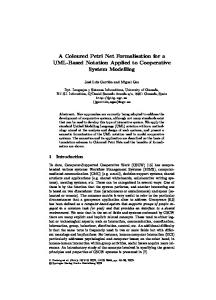
If iδ(z9, t98) and s(rr(v4))=δ(z3, t38). Between v3 and v4 the priority rule π chooses v3. Since transition t98 is enabled by (1) and (2), it fires, then the stamp s(rr(v3)) is set to zero and the marking M2, such that M1[t98()>M2, is the following: M2(z9)=, M2(z8)==, M2(zi)=M1(zi) for each zi∈P with i≠8,9. Figure 4 shows the CTPN at marking M2 and figure 5 shows the corresponding transition digraph that exhibits the cycle γ=({z2, z3, z8, z7,},{e23, e38, e87, e72}) not including z1. Hence, according to Proposition 1 the AGVS is in deadlock condition.
14
z4
, s(rr(v4))= =, 2
UP
UP
t72
, s(rr(v1))=, 0
UP t10,9
z7
Id
z1
UP
Id
Id
z6
UP
, s(rr(v5))=, 5 t10,1 t71 UP Id UP
UP
UP
t65 t9,10
Id
Id
z5
Id
Id
Id
t59
z9 Id
t89
t78
z2
UP
UP
t8 7
t23
t49
Id
Id
Id
, s(rr(v2))= =, 1
t98
UP
Id
z3 UP
t84 UP
Id
UP
Id
z8
UP
t38
Id
UP
, s(rr(v3))=, 0
t10,6
UP
Id
z10
t1,10
t17
Figure 4. The CTPN at marking M2 for Example 4.
z4
z8
z9
v4 z5
z3 v3
v2 z2
z1 v1
z7
z6 z10
Figure 5. Digraph DT for Example 4.
5.
Definition of the control policy This section presents two control policies (CPs) to avoid deadlocks and collisions in zone-
controlled AGVSs. The first CP was introduced by Fanti (2002a) and the second one is defined in this paper. The two policies share the same algorithm checking for zone validation and differ for the path validation algorithm.
15
5.1
Control policy 1 In terms of Petri nets modelling, a transition tim∈T is said to be controlled if its firing is
determined by a CP when tim is enabled according to conditions C1 and C2. Therefore, a CP is a restrictive policy that determines whether a controlled transition can fire on the basis of knowledge of the net state. When a controlled transition tim∈T can fire according to a CP, we say that tim is control enabled under this CP. Moreover, if at least one transition is control enabled, the CTPN is said controlled under this CP. More formally, a CP is a mapping that associates with each event σ∈Σ1∪Σ2 and with each marking M a control action that enables and inhibits event σ, i.e., distinguishing between 1-type and 2-type events: fi : Σi×MA→{0,1} with i=1,2
(5)
where fi(σi,M)=0 (fi(σi,M)=1) means that for the CTPN at marking M event σi is control inhibited (control enabled) for i=1,2. In particular, governing by f2 a 2-type event σ2=v means to control the corresponding transition tim, where ri and rm are the first and the second zones of rr(v). Note that transitions ti1∈T do not require any control, because their occurrence does not determine deadlocks and collisions. From the CTPN point of view, a deadlock means that once some marking has been reached, some colour enabled transitions cannot be fired any longer. The consequence in our model is that the travel of an AGV along a path is interrupted and the vehicle can not reach the docking station. Accordingly, we define task marking the marking associated with the system state in which all the AGVs are in the docking station and have completed their assigned routes. More formally, we introduce the following definition: Definition 1: Marking M* is called task marking if M*(z1)=NV (i.e., NV tokens are in z1 with colour ) and for each zi such that zi≠z1 it holds M*(zi)=. To avoid deadlock it is sufficient to guarantee that each AGV route can continue so that all vehicles can reach the docking station under the control policy. Accordingly, the following definition is given: Definition 2: A CTPN is deadlock-free at marking M∈R(M0) under a CP iff there exists a controlled firing sequence ω so that M[ω>M*. 16
According to Definition 2, the deadlock avoidance controller can be synthesized by finding for the CTPN model a CP that keeps the CTPN deadlock-free, i.e., able to reach the task marking M*. Starting from Proposition 1, a deadlock avoidance policy can be defined in a straightforward manner, on the basis of a look-ahead procedure including just one step (Fanti et al. 1997, Fanti 2002a). More precisely, when an event has to occur, the policy updates the next marking M’, builds the adjacency matrix of the new transition digraph DT(M’) and inhibits the event iff such a digraph contains a cycle not including z1. Such a control policy is defined as follows: fi(σi,M)=0 if the transition digraph associated with M’ and described by the adjacency matrix AM’ exhibits a cycle not including z1. fi(σi,M)=1 elsewhere, with i=1,2. As shown in (Fanti et al. 1997), this control algorithm may lead the system to a situation that is called restricted deadlock. Although the system is not in a deadlock state, in such a condition it inevitably incurs a permanent blocking caused by the control inhibition, therefore the task marking M* is not reached. Since it is shown that the defined CP incurs a restricted deadlock iff a second level deadlock occurs, the defined CP is deadlock free if the necessary condition of Proposition 2 is violated. Hence, the following control policy, named CP1, is deadlock and restricted deadlock free. CP1 Let the CTPN be at time τ and at marking M and denote with M’ the marking obtained from M after the occurrence either of σ1∈Σ1 or of σ2∈Σ2. The restriction policy is defined as follows: f1(σ1,M)=0 if the transition digraph associated to M’ and described by the adjacency matrix AM’ exhibits a cycle that does not include z1 or if Γ2(M’) is not empty and nV(M’)≥(C20(M’)-1). f1(σ1,M)=1 elsewhere. f2(σ2,M)=0 if the transition digraph associated to M’ and described by the adjacency matrix AM’ exhibits a cycle that does not include z1. f2(σ2,M)=1 elsewhere. 17
By Proposition 2, we deduce that if the CTPN is at the initial marking M0 characterized by a transition digraph that does not exhibit a cycle including z1 and if nV(M0)M*. The recalled control policy is the less restrictive policy proposed in Fanti (2002a). We remark that such a policy suffers from high off-line computational complexity. A further disadvantage of CP1 is that the policy permissiveness is considerably diminished by the presence of bi-directional guide-paths in the AGVS layout.
5.2
Control policy 2 To overcome the drawbacks of CP1, we introduce a second control policy based on an
analysis of the task marking reachability. Definition 3: Let the CTPN be at marking M’∈R(M0) and at time τ, and let us suppose that f1(σ1,M)=0 for each σ1∈Σ1 and M∈MA. The task marking M* is said to be reachable from M’ under f2 and the priority rule π, if there exists a controlled firing sequence ω so that M’[ω>M*. In the following we introduce the novel control policy CP2. CP2 Let the CTPN be at time τ and at marking M and let M’ denote the marking obtained from M after the occurrence either of σ1 or of σ2. The restriction policy is defined as follows: f1(σ1,M)=1 if M*is reachable from M under f2 and the priority rule π. f1(σ1,M)=0 elsewhere. f2(σ2,M)=0 if the transition digraph associated to M’ and described by the adjacency matrix AM’ exhibits a cycle that does not include z1. f2(σ2,M)=1 elsewhere. The following proposition proves that the system controlled by CP2 is deadlock and restricted deadlock free. 18
Proposition 3: Let the CTPN be at marking M∈R(M0) at time τ. If M* is reachable from M under f2 and the priority rule π, the CTPN is deadlock free under CP2. Proof Let us suppose that the CTPN is at time τ and at marking M∈R(M0). If we assume that no 1type event occurs, by applying f2 and a priority rule π only one possible firing sequence ω can be obtained to reach marking M*. By assumption such a sequence exists and successively f2 controls the 2-type events inhibiting transitions that determine deadlock at the next step. Moreover, f1 enables a 1-type event if there exists a controlled firing sequence ω under f2 and the priority rule π, so that the CTPN can reach M*. So the AGVS performance will follow the event sequence ω as long as a new 1-type event occurs. Hence, the system deadlock freeness is guaranteed. 6.
Synthesis of the controller This section describes the two activities of the real time controller: the zone validation and
the path validation that implement CP1 and CP2. While the zone validation algorithm is the same for the two policies, CP1 and CP2 differ for the PVA. 6.1
Zone validation
Let us suppose that the CTPN is at marking M and that transition tim is colour enabled, i.e., M(zi)==. If s(rr(v))≥ δ(zi) holds, event σ2=v can occur. In such a case, the controller executes the following Zone Validation Algorithm (ZVA). ZVA A1 If M(zm)≠ by C1) the transition cannot fire, the zone is not validated. Go to step A5. A2 If M(zm)= then the controller determines the new marking: M’(zi)= M’(zm)= M’(z)=M(z) for each z∈P with z≠zm, and z≠zi. A3 The Matrices algorithm provides matrices IM and AM’. A4 A depth-first search algorithm (Reingold et al. 1977) is applied to AM’: if the search finds a cycle not including z1 then f2(σ2,M)=0 and go to step A5, 19
else f2(σ2,M)=1 and go to step A6. A5 The zone is not validated, the behaviour of the AGVS continues with the CTPN at marking M. STOP. A6 The zone is validated and tim fires, the behaviour of the AGVS continues with the CTPN at marking M’. STOP. We remark that Step A1 allows us to avoid collisions and step A4 tests whether marking M’ is a deadlock state or not. 6.2
Path validation The path validation consists in enabling or inhibiting 1-type events in order to avoid
immediate deadlocks and restricted deadlocks as long as a new path is assigned to some vehicle. Let r be the path that the scheduler proposes for vehicle v and let M be the current marking of the CTPN at time τ. Under CP1, the controller executes the following Path Validation Algorithm (PVA). PVA1 B1 Update the marking of the CTPN as follows: M’(zk)= where zk is the first resource of r(v) M’(zi)=M(zi) for each zi∈P with zi≠zk. B2 A depth-first search algorithm is applied to AM’: if the search finds a cycle not including z1 then f1(σ1,M)=0 and go to step B4. B3 Build the path digraph and the second level digraph. If Γ2(M’) is not empty and nV(M’)≥(C20(M’)-1), then f1(σ1,M)=0 and go to step B4, else go to step B5. B4 r(v) is not validated and the evolution of the CTPN continues starting at marking M. STOP. B5 r(v) is validated and the evolution of the CTPN continues starting at marking M'. STOP. Under CP2, the real time controller is to validate the proposed route by using PVA2 which works according to the following steps. PVA2 B1 Update the marking of the CTPN as follows: 20
M’(zk)= where zk is the first resource of r(v) M’(zi)=M(zi) for each zi∈P with zi≠zk. B2 Start a simulation run that under the ZVA and a priority rule π checks that the CTPN reaches marking M* from M’. B3 If marking M* is reached then r(v) is validated and the evolution of the CTPN continues starting at marking M’, else r(v) is not validated and the evolution of the CTPN continues starting at marking M. STOP. 6.3
Some remarks about the computational complexity of the proposed strategies The zone validation activity exhibits the complexity of the depth-first search algorithm
(Reingold et al. 1977), which is polynomial with complexity O(NZ). As shown in Fanti (2002a), PVA1 has a polynomial complexity with the number of cycles 2
D R(M) and DR(M). Since these numbers grow exponentially with the number of nodes of the digraphs, PVA1 may exhibit high complexity. In fact, each bi-directional guide-path corresponds to a first level cycle and each couple of bi-directional guide-paths sharing a node in the digraph representing the system corresponds to a second level cycle (Fanti 2002a). Hence, with reference to figure 1, if all the guide paths in the case study were bi-directional, CP1 would exhibit a high computational complexity, while being severely restrictive. More precisely, in such a case the number of cycles in the first level and second level digraphs would be c1=(NZ-1)!=9! and c2=((NZ-1)!-1)!=(9!-1)! respectively, hence the path validation under PVA1 would require O(9!(9!-1)!) operations (Fanti 2002a). On the other hand, the computational complexity of the proposed control policy CP2 does not depend on the number of cycles in the system layout. In particular, implementing PVA2 requires a simulation run where NVL events can occur (L being the maximum length of each assigned route). For each 2-type event of the simulation, a zone validation must be verified with complexity O(NZ). Moreover, for each 2-type event at most NV zone validations verify whether an inhibited event can be enabled. Summing up, the path validation under PVA2 requires O(NV2LNZ) operations. Hence, with reference to the layout in figure 1, regardless of the number of bidirectional guide-paths, it holds NZ=10 and assuming NV=5 and L=2NZ=20 we get 5·103 operations.
21
7.
Simulation study This section presents a simulation study performed for the AGVS described in Example 1
employing in turn the control policies CP1 and CP2. The aim of the present investigation is to compare the effectiveness of CP2 with CP1 by means of appropriate performance measures. Additionally, in the simulations the AGV fleet size is varied, in order to check the control policy effectiveness when traffic changes from low to medium and finally becomes intense. The CTPN representing the system is implemented in the MATLAB-Stateflow environment (The MathWorks Inc. 1997), where it is possible to integrate modelling and simulation of Stateflow event-driven systems (e.g., the AGVS dynamics) with the execution of MATLAB computation routines (e.g., developing the ZVA and PVA algorithms), while keeping track of time by way of a software clock. The rationale for choosing MATLAB-Stateflow as simulation environment, rather than more evolved and specific software, e.g. such as Arena (Kelton et al. 1998), lies in its simplicity and immediacy. In fact, rather than mimicking the operation of an actual AMS in its complexity (workstations, buffers working procedures, etc.), the purpose of the following simulation study is testing the efficiency of several traffic control policies. Hence, we investigate, for equivalent settings, which policy restricts the system congestion while guaranteeing that the vehicles moving in the system reach their destination at an early time. Summing up, our purpose is to simulate the CTPN while assigning the vehicles the longest and most varied paths. To this aim, MATLAB exhibits two convenient features: 1) simplicity of implementation and ability to reproduce the CTPN modularity and structure; 2) possibility to execute, when required, a simulation run implementing PVA2. On the contrary, using a software environment such as Arena to reproduce the CTPN would require the implementation of computationally intensive cycles, e.g. in C++ code, in order to execute a simulation run during the system evolution. A detailed discussion of the MATLAB-Stateflow AGVS model is beyond the scope of this paper, nevertheless in the sequel we briefly describe the model rationale, since the execution of the CTPN dynamics in MATLAB-Stateflow is carried out by a novel implementation technique. More precisely, here the Petri net places are represented by a finite state automaton, with sub-states modelling the zone shift of the AGV currently under investigation by the AGVS management system. For sake of brevity, we do not show the details of such technique. However, figures 6 and 7 show the MATLAB-Stateflow models implementing the AGVS controlled by restriction policies CP1 and CP2, respectively. Both charts in figures 6 and 7 comprise three main subsystems: “AGVS Dynamics”, “Buffer” and “PVA”. Note that 22
the first two blocks are nearly the same in both machines, on the contrary the last block differs since it implements in turn PVA1 and PVA2. More precisely, the “AGVS Dynamics” block handles the vehicle travels in the system and it is composed of two procedures: “Place” and “Vehicle Moves and ZVA”. Now, the first procedure describes the generic CTPN place, i.e., a generic zone; the second one is in charge of selecting the next vehicle to move and executing ZVA for the selected AGV. Moreover, the “AGVS Dynamics” block updates and stores the current marking of the CTPN. When a new route is proposed, the “Buffer” block is invoked. Indeed, it saves the current CTPN marking while PVA validates a new path proposed by the “Vehicle Moves and ZVA” block, transferring the system data to the PVA block in order to validate the new route. In addition, the “Buffer” block restores the system status in case of path rejection, hands the target marking over in case of route authorization and informs the “AGVS Dynamics” block about the path validation outcomes. Finally, the “PVA” block performs the path validation and notifies its decisions to the “Buffer” block. As already mentioned, the PVA implementation differs for the two restriction policies considered. In particular, the “PVA1” block (see figure 6) tests the occurrence of a restricted deadlock by checking the presence of a particular cycle in the second level digraph originating from the new marking, according to Proposition 2. Instead, in the implementation of PVA2 (see figure 7) the “PVA2” block tests whether Proposition 3 holds by performing a simulation of the AGVS in order to check the task marking reaching under the ZVA control and supposing that no 1-type event occurs. This test is accomplished by an additional “AGVS Dynamics” sub-block that simulates the AGVS behaviour originating from the marking under consideration. To sum up, we remark that using the MATLAB-Stateflow environment to implement the AGVS under study results in a compact and modular model, in which it is easy to modify the PVA implementation. Indeed, the system model is always the one represented in figure 6 (figure 7) when PVA1 (PVA2) is employed, no matter how many zones the AGVS comprises. In fact, in the automaton implementing the system a single state represents the generic CTPN place and few changes are necessary to update the system layout and the possible routes.
23
Figure 6. The MATLAB-Stateflow machine implementing the CTPN under CP1.
Figure 7. The MATLAB-Stateflow machine implementing the CTPN under CP2.
24
7.1
Description of the simulation experiments Several simulation experiments are conducted for Example 1 under the following
assumptions, employing in turn CP1 and CP2. A set of 300 routes resulting in three replications of a set of 100 paths, all starting and terminating with the docking station z1, is considered for the AGVS to accomplish in a predetermined order. The maximum route length is set equal to ten, i.e., each route proposed by the path scheduler consists of ten zones, all ending with z1. The assigned set of 300 routes is considered in six experiments for both control policies with an AGV fleet size NV ranging from 2 to 7. In order to keep into account the time necessary for an AGV to travel from a zone to an adjacent one, i.e., the time for a vehicle to move along a guide-path or accomplish a load (unload) operation from (to) a workstation or the corresponding buffer, we set a time for a vehicle to accomplish such zone crossing. For sake of simplicity, we assume that any AGV can travel between any couple of adjacent zones in 200 time units, i.e., in a time interval equal to the 500th part of the total run time. The priority rule selected for the simulation experiments is the FCFS policy formally defined by (4). Since simulation experiments employing a different number of vehicles and a different restriction policy may not require the same run time to accomplish the 300 selected missions, a fixed run period of T=100,000 time units is considered. Finally, in the present case study we assume that resources are reliable. Nevertheless, we remark that if a truck breakdown occurs, the failed vehicle is removed from the AGVS layout and the system dynamics proceeds with its evolution using a lower fleet size and by assigning a new marking to the CTPN. 7.2
Performance measures In order to compare the effectiveness of the two control strategies in assigning the
transport tasks to the AGVS, as well as to facilitate selection of the AGV fleet size, we consider several performance measures for the system. For each simulation experiment, we select as measure of performance the number of routes completed by the AGV fleet under the ZVA and PVA verifications (throughput) in the run time T. Clearly, the number of completed missions is an index of the traffic management policy effectiveness in having the system accomplish paths while minimizing blockings. Note that only completed missions are considered in the throughput computation: at completion of the run time unfinished tasks are discarded. 25
In addition, vehicles utilization is evaluated in the simulations. The operative conditions in which the generic vehicle activity can be classified are as follows. (i)
Loaded and booked travel – the vehicle is accomplishing a mission. This state comprises two sub-states: the AGV is either booked and travelling empty toward the loading zone, or transporting a piece toward the assigned unloading area.
(ii)
Blocked – the AGV, while travelling loaded or booked, is blocked in a zone by the control system in order to avoid deadlock or collision.
(iii)
Empty and available – the vehicle, after unloading a part at the destination zone, is either empty and travelling towards the docking station or idle in the docking station waiting for destination. At both stages the AGV can receive the next transportation task by the path scheduler.
The measure of performance adopted for vehicles activity is the average percentage time a vehicle spends in each of the above three states. Additionally, we consider vehicles utilization, computed as the average percentage time a vehicle spends executing a mission, i.e., being in states (i) or (ii). 7.3
Simulation results Results of the simulation experiments are summarized in figures 8-12. In particular, the
AGVS throughput is depicted in figure 8 and reported in detail in tables 1 and 2 for CP1 and CP2, respectively, when using different AGV fleet sizes. Figure 8 shows that the AGVS throughput reaches the maximum value under CP1 when five vehicles are available, whereas the highest number of accomplished transportation tasks is obtained under CP2 with six vehicles. Moreover, it can be inferred from figure 8 that under both PVA strategies the transportation system is inefficient for a modest AGV fleet size, since the number of vehicles is small compared both with the AMS size and the large number of tasks to be completed in the assigned run time. All the same, under both real time control strategies the homogeneous increase of the allocated missions (see figure 8) is an obvious consequence of the growth of the available AGVs number (Rajotia et al. 1998b). However, the throughput value reaches a maximum for a given fleet size, since traffic becomes congested and vehicles are often blocked in order to avoid deadlock and collisions. For all AGV fleet sizes CP2 provides better throughput values than CP1. The AGVS throughput is reported in detail under CP1 (see table 1) and CP2 (see table 2). Each column in tables 1 and 2 shows the simulation results under the selected CP for a specific fleet size NV ranging from 2 to 7, reporting the number of transportation missions 26
accomplished by each vehicle and the tasks completed by the whole AGV fleet in the run time. Comparing the corresponding columns in table 1 and table 2, i.e., the results of the simulation runs with the same fleet size, the improvement in the overall number of completed transportation tasks under CP2 is apparent. Clearly, CP2 allows a larger number of completed missions than CP1, because PVA2 is less restrictive than PVA1. More precisely, PVA1 inhibits some paths because it detects the potential occurrence of restricted deadlock in the future. On the contrary, in some of these cases PVA2 shows by simulation that the mission can be completed if the AGVS follows a particular events sequence. The average percentage time of loaded and booked travel under both CPs is reported in figure 9. Again, CP2 leads to better results, exhibiting for any number of vehicles a performance index that is always higher than the one computed with the alternative restriction policy. However, under both techniques such an index decreases with the increase in AGV fleet size: this is expected, because of the traffic congestion deriving from the large number of travelling vehicles in the AGVS. Figure 10 depicts the average percentage blocked time of vehicles. Again, it is observed that CP2 outperforms CP1. Moreover, for both techniques the performance index increases with the fleet size. Indeed, the probability that a vehicle is blocked while executing a transportation task becomes higher when the system is overcrowded. The average empty and available time is reported in figure 11. Such an index is only partly dependant on the adopted control policy: in fact, it is greatly influenced by the selected dispatch policy and by the transport request rate. As previously mentioned, investigating the path scheduler is not the purpose of the present paper, therefore we assume that the issue of assigning a proper succession of missions to the vehicles has been addressed. Despite such dependence of this index on the dispatch policy, we can observe that CP2 outperforms CP1 again. In fact, the path validation algorithm based on the task marking reaching tends to reject a lower number of tasks than the algorithm based on cycles detection in the digraphs associated to the AGVS. Finally, the AGVS utilization index is reported in figure 12. Here, the average percentage time a vehicle is either booked travelling toward a loading station, or loaded and blocked, or else carrying a piece towards its destination is reported. This performance index is high for both techniques, since most of the time the vehicles are busy accomplishing a mission out of the docking station and a task may be assigned to an AGV as soon as it finishes a mission and starts travelling to the docking station. Nevertheless, CP2 outperforms CP1 again for any number of vehicles in the system, in accordance with the results previously described. In other 27
words, the path validation controller of CP2 is able to validate a larger number of missions than CP1, so that the vehicles are utilized most of the time. As a summary of the adopted control policies performance, the distribution of the vehicles activity time is depicted in figures 13 and 14 under CP1 and CP2, respectively. For both techniques we observe the same time indices trends with respect to a variation in the AGV fleet size. However, the improvement resulting from the use of CP2 is apparent from a comparison of figures 13 and 14. Under CP2 for any number of vehicles in the system the average engaged travel percentage time is greater than the other time indices (see figure 14). On the contrary, under CP1 the decrease rate of the average engaged travel percentage time is higher than under CP2, so that the index becomes lower than the average time spent by the vehicles in the blocking states when the system is congested (see figure 13). Accordingly, under CP2 the system is less prone to blockings than under CP1. For instance, if we consider the simulation run with six vehicles when adopting CP2, approximately 59.5% of the overall run time is employed by the AGVs travelling busy while accomplishing a task. The average percentage time between accomplishment of a mission and assignment of the next task to the same vehicle equals a satisfactory 4.9%, confirming the policy efficiency. The remaining 35.6% time is occupied by blockings, therefore vehicles are often stalled in order to avoid deadlocks or collisions. Clearly, such a considerable value of the last index partly depends on the adoption of the zone control methodology when managing the vehicles dynamics. On the other hand, it can be remarked that the high system throughput (265 tasks assigned out of the available 300, see table 1) in the total run time balances such an inconvenience. 7.4
Some remarks on the applicability of the proposed traffic control technique
We showed that the CP2 control strategy outperforms CP1 both in terms of throughput and vehicles utilization. Nevertheless, in order to apply CP2, it is crucial to test its effectiveness in real time. In other words, all moves and mission acceptances or refusals must be executed on line, i.e., in a response time that can be neglected. More precisely, all decisions performed by the real time controller are classified either as zone validations or as path validations. The first type of decisions are executed by ZVA by detecting cycles in the transitions digraph and can be easily implemented on line by way of a depth-first search algorithm in polynomial time (see section 6.3). Now, because of the high computational complexity of PVA1, its application can be impracticable when the system layout is complex. On the contrary, PVA2 takes decisions executing a simulation testing the task marking reaching and such a check is performed in polynomial time (see section 6.3). 28
Two issues must be enlightened. First, it is important for the implementation of PVA2 that the controller keeps memory of the succession of the 2-type events as obtained by the simulation run: hence, when a route is validated, the AGVS dynamics must follow the behaviour forecasted by the simulation till a new route is validated. Second, the simulation results and conclusions hold both under deterministic and stochastic transition times. In any case, it is crucial that the controller stores the succession of events occurred during the simulation run, so that the AGVS follows the forecasted events sequence. In the present work we focus on the deadlock avoidance policy performance, hence we make use of the MATLAB interpreted language in order to perform a simulation run (i.e., the PVA2 implementation) in a simulated environment. However, the possible implementation of the actual controller in an industrial setting may be simply and more rapidly carried out by executing a custom code on a central processing unit connected to appropriate sensors. In fact, it is essential for the on-line applicability of the proposed deadlock avoidance policy that such a simulation is performed in real time. In other words, after accomplishing the PVA2 algorithm, the AGVS must still be in the state previous to the path validation, otherwise the simulation does not mirror the authentic system dynamics and the corresponding decisions apply to a system state preceding the actual one. As an example, consider the complex network representation of the Delphi-Harrison layout reported by Oboth et al. (1999), with NV=7 vehicles and NZ=219 zones. Assuming that the maximum possible length of each assigned route is L=2NZ, for such a system PVA2 requires the execution of about 5·106 operations in real time (see section 6.3). Hence, a commercial personal computer featuring a 2 GHz CPU performs such a number of elementary operations in much less than 1 second. Now, a commercial AGV may reach the speed of 1 m s-1, hence the time required by the decision does not slow down the system operation.
29
280 CP1
No. of Routes Completed
260
CP2
240 220 200 180 160 140 2
3
4
5
6
7
AGV Fleet Size
Figure 8. Throughput for various AGV fleet sizes.
AGV no. 1 2 3 4 5 6 7 TOTAL
2 AGVs No. of tasks 79 69 148
3 AGVs No. of tasks 71 55 59 185
4 AGVs No. of tasks 51 54 52 48 205
5 AGVs No. of tasks 41 44 44 47 34 210
6 AGVs No. of tasks 41 28 33 31 33 31 197
7 AGVs No. of tasks 33 26 22 28 24 30 36 199
Table 1. Detailed results of AGVS throughput for various AGV fleet sizes under CP1.
AGV no. 1 2 3 4 5 6 7 TOTAL
2 AGVs No. of tasks 72 76 148
3 AGVs No. of tasks 67 64 67 198
4 AGVs No. of tasks 65 49 61 60 235
5 AGVs No. of tasks 56 52 51 56 48 263
6 AGVs No. of tasks 47 44 41 46 48 39 265
7 AGVs No. of tasks 36 33 37 36 42 32 41 257
Table 2. Detailed results of AGVS throughput for various AGV fleet sizes under CP2. 30
Average Time AGVs Loaded and Booked Travel [%]
110,0 CP1 100,0
CP2
90,0 80,0 70,0 60,0 50,0 40,0 30,0 2
3
4
5
6
7
AGV Fleet Size
Figure 9. Average time vehicle loaded and booked travel for various AGV fleet sizes.
56,0 CP1
Average Time AGVs Blocking [%]
51,0
CP2
46,0 41,0 36,0 31,0 26,0 21,0 16,0 11,0 6,0 2
3
4
5
6
AGV Fleet Size
Figure 10. Average time vehicle blocking for various AGV fleet sizes.
31
7
Average Time AGVs Empty and Available [%]
8,0 CP1 CP2
7,0 6,0 5,0 4,0 3,0 2,0 1,0 2
3
4
5
6
7
AGV Fleet Size
Figure 11. Average time vehicle empty and available for various AGV fleet sizes.
100,0 CP1
Average Time AGVs Utilization [%]
99,0
CP2
98,0 97,0 96,0 95,0 94,0 93,0 92,0 91,0 90,0 2
3
4
5
6
AGV Fleet Size
Figure 12. Average time vehicle utilization for various AGV fleet sizes.
32
7
100,0 Loaded and Booked Travel
90,0
Blocked
80,0
Empty and Available Average Time [%]
70,0 60,0 50,0 40,0 30,0 20,0 10,0 0,0 2
3
4
5
6
7
AGV Fleet Size
Figure 13. Vehicle activity average time under PVA1.
100,0 Loaded and Booked Travel
90,0
Blocked 80,0
Empty and Available
Average Time [%]
70,0 60,0 50,0 40,0 30,0 20,0 10,0 0,0 2
3
4
5
6
AGV Fleet Size
Figure 14. Vehicle activity average time under PVA2.
33
7
8 Conclusions This paper proposes a Coloured Timed Petri Net (CTPN) model and an efficient control strategy to avoid deadlock and collisions in zone-controlled Automated Guided Vehicle Systems (AGVSs). The peculiarity of the resulting model consists in its modularity, so that the structure of the CTPN can be automatically built and easily updated if the system layout changes. Moreover, the assigned paths, i.e., the token colours, are modified as the vehicles move from zone to zone or a new route is assigned. In addition, the proposed control strategy can be easily applied and improves both the permissiveness in zone acquisition and the computational complexity of the traffic management strategies proposed by one of the authors (Fanti 2002a). More precisely, we modify the Path Validation Algorithm (PVA) that checks the assignment of the new missions to vehicles in order to guarantee the success of all the AGV assigned travels. Such a validation is performed in polynomial time by a simulation run forecasting the AGVS behaviour. Several simulation experiments performed for an AGVS with varying fleet size show the effectiveness of the proposed control strategy compared to a policy previously suggested. To this aim, we propose a MATLAB-Stateflow environment that is suitable to reproduce the modularity of the CTPN and can be an efficient tool to implement the proposed PVA in the AGVS shop floor. Future research has to investigate how the integration of the proposed deadlock avoidance strategy with the existent scheduling policies affects the AGVS performance.
REFERENCES ASHAYERI, J., GELDERS, L. F., and VAN LOOY, P. M., 1985, Micro- computer simulation in design of automated guided vehicle systems. Material Flow, 2(1), 37-48. BANASZAK, Z. A., and KROGH, B. H., 1990, Deadlock Avoidance in Flexible Manufacturing Systems with Concurrently Competing Process Flows. IEEE Transactions on Robotics and Automation, 6(6), 724-734. BLAIR, E. L., CHARNSETHIKUL, P., and VASQUES, A., 1987, Optimal routing of driverless vehicles in a flexible material handling system. Material Flow, 4(1+2), 73-83. CHO, H., KUMARAN, T. K., and WYSK, R. A., 1995, Graph-Theoretic Deadlock Detection and Resolution for Flexible Manufacturing Systems. IEEE Transactions on Robotics and Automation, 11(3), 413-421. CHU, F., and XIE, X., 1997, Deadlock analysis of Petri nets using siphons and mathematical programming. IEEE Transactions on Robotics and Automation, 13(6), 793-804. CO, G.C., and TANCHOCO, J.M.A., 1991, A review of research on AGVS vehicle management. Engineering Costs and Production Economics, 21, 35-42. DESROCHERS, A. A., and AL-JAAR, R. Y., 1995, Applications of Petri Nets in Manufacturing Systems. (New York: IEEE Press). EGBELU, P. J., and TANCHOCO, J. M. A., 1984, Characterization of automatic guided vehicle dispatching rules. International Journal of Production Research, 22(3), 359-374.
34
EGBELU, P. J., and TANCHOCO, J. M. A., 1986, Potentials for bi-directional guide-path for automated guided vehicle based systems. International Journal of Production Research, 24(5), 1075-1097. EZPELETA, J., COLOM, J. M., and MARTINEZ, J., 1995, A Petri Net Based Deadlock Prevention Policy for Flexible Manufacturing Systems. IEEE Transactions on Robotics and Automation, 11(2), 173-184. EZPELETA, J., and COLOM, J. M., 1997, Automatic synthesis of colored Petri net for the control of FMS. IEEE Transactions on Robotics and Automation, 13(2), 327-337. FANTI, M. P., MAIONE, B., MASCOLO, S., and TURCHIANO, B., 1997, Event Based Feedback Control for Deadlock Avoidance in Flexible Production Systems. IEEE Transactions on Robotics and Automation, 13(3), 347-363. FANTI, M. P., MAIONE, B., and TURCHIANO, B., 2000, Comparing Digraph and Petri Net Approaches to Deadlock Avoidance in FMS. IEEE Transactions on Systems, Man and Cybernetics. Part B: Cybernetics, 30(5), 783-798. FANTI, M. P., MAIONE, G., and TURCHIANO, B., 2001, Distributed event-control for deadlock avoidance in automated manufacturing systems. International Journal of Production Research, 39(9), 1993-2021. FANTI, M. P., 2002a, Event-based controller to avoid deadlock and collisions in zone control AGVS. International Journal of Production Research, 40(6), 1453-1478. FANTI, M. P., 2002b, Deadlock-Free Control in Automated Guided Vehicle Systems. In P. Ezhilchelvan and A. Romanovsky (eds.), Concurrency in Dependable Computing (The Netherlands: Kluwer Academic Publishers). FELDMANN, K., and COLOMBO, A.W., 1998, Material Flow and Control Sequence Specification of Flexible Systems Using Coloured Petri Nets. International Journal of Advanced Manufacturing Technology, 14(10), 760-774. HARARY, F., 1971, Graph Theory, (Reading: Addison-Wesley Publishing Company). HSIEH, F.S., and CHANG, S. C., 1994, Dispatching-Driven Deadlock Avoidance Controller Synthesis for Flexible Manufacturing System. IEEE Transactions on Robotics and Automation, 10(2), 196-209. HSIEH, S., 198, Synthesis of AGVS by Coloured-Timed Petri Nets. International Journal of Computer Integrated Manufacturing, 11(4), 334-346. HUANG, Y., JENG, M., XIE, X., and CHANG, S., 2001, Deadlock prevention policy based on Petri nets and siphons. International Journal of Production Research, 39(2), 283-305. JENSEN, K., 1992, Colored Petri Nets, Basic Concepts, Analysis methods and Practical Use, Vol I, EATS Monography and Theoretical Computer Science (New York: Springer Verlag). JIANG, Z., ZUO, M. J., FUNG, R. Y. K., and TU, P. Y., 2000, Temporized coloured Petri nets with changeable structure (CPNCS) for performance modelling of dynamic production systems. International Journal of Production Research, 38(8), 1917-1945. KELTON, W. D., SADOWSKI, R. P., and SADOWSKI, D. A., 1998, Simulation with Arena. (Boston: Mc Graw-Hill). KIM, C. W., and TANCHOCO, J. M. A., 1991, Conflict-free shortest bi-directional AGV routing. International Journal of Production Research, 29(12), 2377-2391. KUMARAN, T. K., CHANG, W., CHO, H., and WYSK, R. A., 1994, A structured approach to deadlock detection, avoidance and resolution in flexible manufacturing systems. International Journal of Production Research, 32(10), 2361-2379. LAWLEY, M. A., REVELIOTIS, S. A., and FERREIRA, P. M., 1998, A correct and scalable deadlock avoidance policy for flexible manufacturing systems. IEEE Transactions on Robotics and Automation, 14(5), 796-809. LAWLEY, M. A., 2000, Integrating flexible routing and algebraic deadlock avoidance policies in automated manufacturing systems. International Journal of Production Research, 38(13), 2931-2950. LEE, C. C., and LIN, J. T., 1995, Deadlock prediction and avoidance based on Petri nets for zone-control automated guided vehicle systems. International Journal of Production Research, 33, 3249-3265. MOORE, K. E., and GUPTA, S. M., 1996, Petri Net Models of Flexible and Automated Manufacturing Systems: a Survey. International Journal of Production Research, 34(11), 3001-3035. NANDULA, M., and DUTTA, S. P., 2000, Performance evaluation of an auction-based manufacturing system using coloured Petri nets. International Journal of Production Research, 38(9), 2155-2171.
35
OBOTH, C., BATTA, R., and KARWAN, M., 1999, Dynamic Conflict-free routing of automated guided vehicles. International Journal of Production Research, 37(9), 2003-2030. RAJOTIA, S., SHANKER, K., and BATRA, J. L., 1998, A semi-dynamic time window constrained routeing strategy in an AGV system. International Journal of Production Research, 36(1), 35-50. RAJOTIA, S., SHANKER, K., and BATRA, J. L., 1998, An heuristic for configuring a mixed uni/bidirectional flow path for an AGV system. International Journal of Production Research, 36(7), 1779-1799. REINGOLD, E. M., NIEVERGELT, J., and DEO, N., 1977, Combinatorial Algorithms. Theory and Practice. (New Jersey: PrenticeHall). REVELIOTIS, S. A., and FERREIRA, P. M., 1996, Deadlock Avoidance Policies for Automated Manufacturing Cells, IEEE Transactions on Robotics and Automation, 12(6), 845-857. REVELIOTIS, S. A., LAWLEY, M. A., and FERREIRA, P. M., 1997, Polynomial Complexity deadlock Avoidance Policies for Sequential Resource Allocation Systems. IEEE Transactions on Automatic Control, 42(10), 1344-1357. REVELIOTIS, S. A., 2000, Conflict resolution in AGV Systems. IIE Transactions, 32, 647-659. THE MATHWORKS INC., 1997, Stateflow User’s Guide Version 4. VISWANADHAM, N., NARAHARI, Y., and JOHNSON, T. L., 1990, Deadlock avoidance in flexible manufacturing systems using petri net models. IEEE Transactions on Robotics & Automation, 6(6), 713-722. VISWANADHAM, N., and NARAHARI, Y., 1992, Performance Modeling of Automated Manufacturing Systems. (Englewood Cliff, NJ: Prentice Hall). WALKER, S. P., PREMI, S. K., BESANT, C. B., and BROADBENT, A. J., 1985, The Imperial College free-ranging AGV (ICAGV) and scheduling system. S.E. Andersson (ed.), Proceedings of the 3rd International Conference on Automated Guided Vehicle Systems, Stockholm, Sweden, 189-198. WU, N., and ZHOU, M.C., 2001, Avoiding deadlock and reducing starvation and blocking in automated manufacturing systems. IEEE Transactions on Robotics and Automation, 17(5), 657-668. WU, N., and ZENG, W., 2002, Deadlock avoidance in an automated guidance vehicle system using a coloured Petri net model. International Journal of Production Research, 40(1), 223-238. WYSK, R. A., YANG, N. S., and JOSHI, S., 1991, Detection of Deadlocks in Flexible Manufacturing Cells. IEEE Transactions on Robotics and Automation, 7(6), 853-859. XING, K. Y., HU, B. S., and CHEN, H. X., 1996, Deadlock avoidance policy for Petri net modeling of flexible manufacturing systems with shared resources. IEEE Transactions on Automatic Control, 41(2), 289-295, 1996. YEH, M. S. and YEH, W. C., 1998, Deadlock prediction and avoidance for zone-control AGVS. International Journal of Production Research, 36(10), 2879-2889 ZENG L., WANG, H. P., and JIN, S., 1991, Conflict Detection of Automated Guided Vehicles. International Journal of Production Research, 29(5), 865-879.
36