Hybrid Mutation Particle Swarm Optimisation Method for Available Transfer Capability Enhancement H. Farahmand1, M. Rashidinejad2 A.A. Gharaveisi2, A. Mousavi3, M.R. Irving3, and G.A. Taylor3 1
SINTEF Energy Research, Trondheim, Norway (
[email protected]) 2 Shahid Bahonar University of Kerman, Kerman, IRAN 3 Brunel Institute of Power Systems (BIPS), Electronic and Computer Engineering, School of Engineering and Design, Brunel University, UK
ABSTRACT: A Hybrid Mutation Particle Swarm Optimisation (HMPSO) technique for improved estimation of Available Transfer Capacity (ATC) as a decision criterion is proposed in this paper. First, this is achieved by comparing a typical application of the Particle Swarm Optimisation (PSO) technique with conventional Genetic Algorithm (GA) methods. Next, a multi-objective optimisation problem concerning optimal installation and capacity allocation of Flexible AC Transmission Systems (FACTS) devices is presented and demonstrated. Modern heuristic techniques such as PSO have been demonstrated to be suitable approaches in solving non-linear power system problems. The outcome of this research further demonstrates that with better utilisation of FACTS devices, it is possible to improve transmission capabilities. The motivation of this research is a direct consequence of the deregulation of electricity industries and power markets worldwide. The current deregulated environment provides transmission systems operators (TSO) with more options when procuring transmission services. The effectiveness of the proposed algorithm is demonstrated across a range of case studies, and the results are validated through analyses conducted on IEEE 30-bus and 57-bus test systems. 1
INTRODUCTION
The liberalisation of electricity markets has created the need for researchers and practitioners to put forward better power systems optimisation techniques [1]. The open access to transmission networks enables international involvement in the global electrical power supply markets. The market forces and resultant squeeze on profit margins demand better utilisation of the existing transmission facilities [2,3]. Improvements to Available Transfer Capability (ATC) in power transmission systems are constrained by relatively low voltages and heavily loaded circuits and buses. FACTS devices offer a versatile alternative to conventional reinforcement methods through increased flexibility, lower cost and reduced environmental impacts. They provide new control facilities, both in steady state power flow control and dynamic stability control. Static VAr Compensator (SVC) and Thyristor Controlled Series
1
Compensator (TCSC) are the popular FACTS devices for effective parallel and series compensation in order to enhance ATC. The capacity of transmission equipment can be improved without resorting to costly installation of new transmission networks. This can be achieved by prudent deployment of FACTS devices in the transmission system [4, 35]. The deployment of series and parallel reactive compensators would improve ATC. Typically an optimisation method determines the capacity and the location of these compensators [5, 36]. The multi objective optimisation problem that deals with deployment of FACTS devices in a network is able to handle conflicting objectives at different power system operation modes. The objectives in this paper include ATC enhancement, voltage profile improvement and active power losses reduction. Moreover, the objectives are constrained by power flow limits, network reliability and system security [3,6]. Particle Swarm Optimisation (PSO) [7, 37] is applied in this paper to solve the problem of installation and capacity allocation of FACTS devices in the power transmission network. Over the last decade, PSO algorithms have been successfully deployed in power system optimisations studies [8-12, 38]. One of the advantages of PSO is the capability of particles to share information among each other. For example, during a search process the particles can benefit from the discoveries and previous experiences of all other particles with solution information in the system, which in turn leads to higher overall solution speed. However, due to the multimodality of the objective function, the former advantage could seriously harm the search for a global optimal solution. The multi objective function may also degrade the diversity criteria of the algorithm, and reduce the global searching capability of the PSO algorithm [13]. In order to overcome this weakness and improve the overall solution process, a novel Hybrid Mutation PSO (HMPSO) method consisting of a standard PSO method and a new mutation operator is proposed in this paper. The proposed hybrid method combines fuzzy logic and the Analytical Hierarchy Process (AHP) to model the qualification of each problem objective [28], and prioritise of the objectives. The fitness evaluation applies the velocity of each particle to the global optimum point. A mutation operator that initiates artificial diversification in the particle population is embedded in the PSO to prevent premature convergence to a local optimum. In the following section, the definition of the problem and the resultant mathematical formulation is discussed. In section 3, an introduction to PSO and the novel HMPSO method is given. In section 4, the model is validated across a range of case studies followed by analysis of results. Section 5, outlines the concluding remarks. 2
PROBLEM DEFINITION AND MATHEMATICAL MODELLING
This research focuses on a multi-objective optimisation problem. The problem is formulated in order to find the best location and capacity of FACTS devices. The objective function includes the enhancement of Available Transfer Capability (ATC), the maintenance of the voltage profile and minimisation of active power losses. 2.1
PROBLEM DEFINITION AND MODELLING
The most important goal is to enhance ATC with respect to the economical constraints
2
of a typical interconnected network. In order to achieve this goal, a formal definition of ATC as well as its role in power system operation and control is presented in the first step. Available Transfer Capability According to the North American Electric Reliability Council (NERC), ATC is the difference between Total Transfer Capability (TTC) and the summation of the Existing Transmission Commitment (ETC), the Transmission Reliability Margin (TRM) and the Capacity Benefit Margin (CBM) [15]: 2.1.1
ATC=TTC-( ETC+ TRM +CBM)
(1)
The TTC is the largest transfer increase between the selected source and sink with no violation of any security constraints or contingency [14]. In order to calculate the TTC, the thermal and voltage limits are also considered. The three most practical and popular methods for calculating TTC are: i. Repeated Power Flow (RPF) method [15]. ii. Continuation Power Flow (CPF) method [16]. iii. Security Constrained Optimal Power Flow (SCOPF) method [17]. The method adopted in this research to calculate TTC is based on a simple implementation of the RPF method, which is a suitable method for large-scale power systems in comparison with the other methods [4]. The RPF method needs to trace PV curve up to the nearest distance to the ‘nose’ point (at the nose point the RPF method will diverge). This offers the possibility of considering voltage stability in TTC calculation. In accordance with the RPF method, the system load and power generation will be increased by a specified rate. The power increase continues until at least one of the system constraints related to TTC are violated. Variations in the real power generation and demand of each bus are shown in Equations (2) and (3). PGi = PGi (1 + λk Gi ) PDi = PDi (1 + λk Di )
(2) (3)
Where: PGi : increased real power generation at bus i PGi :
original real power generation at bus i
PDi : increased real load demand at bus i. : original real load demand at bus i. PDi λ: scalar parameter. k Gi : constant rate of changes in generation as λ varies. k Di : constant rate of changes in load as λ varies. The reactive power demand (QD) is also increased in accordance to fix the power factor for all loads.
3
Therefore, TTC can then be calculated using the Equation (4). The equation shows the maximum loadability of an electric power system before reaching the voltage collapse point along with the maximum exchange flows on interfaces, which have not violated the capacity limitation. Thereby, voltage limits and thermal limits are considered in TTC calculation. The TTC calculation is based on static consideration and does not account for the dynamic stability limitations. = TTC min (∑ PDi (λmax ) − ∑ PDia ), ∑ PMaxij (4) i∈k ij∈Tie Lines i∈k Where,
∑P i∈k
Di
(λmax ) is the sum of the load in sink area at λ = λ max , ∑ PDio is the sum of
the load in sink area when λ = 0 , and
∑
ij∈Tie Lines
i∈k
PMaxij is the sum of tie-lines capacity
between the send and the sink area. The existing committed transmission (ETC) is calculated using the power flow calculation. The transmission reliability margin (TRM) is treated as a constant percentage (i.e. 10%) of the TTC. The capacity benefit margin (CBM) can be based on the market value between energy contractors. For the sake of simplicity, CBM is assumed to be zero. Based on the above assumptions, ATC can be estimated by the Equation (5). ATC = TTC − ETC − TRM =− (1 k )TTC − ETC
(5)
Where, k is a predefined percentage of the calculated TTC. Voltage profile and active power losses are calculated using the power flow solution. Static VAr Compensator (SVC) Model In the steady state case, an SVC can be modelled as a reactive power injection/absorption illustrated in Equation (6) [18]:
2.1.2
QSVC = Vt (Vt − Vref ) X SL
(6)
Where: XSL is the voltage control, Vt is the terminal voltage and Vref is the reference voltage. Equation (7) can be used as the alternative representation of Equation (6):
QSVC = BSVC × Vref
2
(7)
Here the value of BSVC varies between the minimum and the maximum capacitive and inductive susceptance. This range is more than the desired reactive power that can be maintained. Thyristor Controlled Series Compensator (TCSC) Model Transmission lines are generally modelled using the classical π model with lumped parameters. The series compensator TCSC is a static capacitor or reactor with an impedance of jXc as shown in Figure 1. 2.1.3
4
Figure 1- Equivalent Circuit of Line with TCSC The difference between the line susceptance before and after the inclusion of a TCSC can be expressed as Equation (8)[19]. Δy ij = y ′ij − y ij = (g ij + jb ij ) ′ − (g ij + jb ij )
(8)
Where: rij g ij = 2 2 rij + x ij
g ′ij =
rij 2 2 rij + (x ij + x c )
x ij b ij = − 2 2 rij + x ij
and
x ij + x c b′ij = − 2 2 rij + (x ij + x c )
and
By deployment of a TCSC between Bus i and Bus j in a power system, the admittance matrix Ybus can be modified as follows:
′ = Ybus Ybus
2.2
0 0 0 y ij ∆ 0 0 + ... ... 0 0 − ∆ y ij 0 0 0
0
...
0
0
0
...
0
...
0 0
− ∆y ij 0
... ... ... 0
...
0
0 0
... ...
0 0
... 0 ∆y ij 0
0 0 0 ... 0 0 0
(9)
THE MATHEMATICAL FORMULATION
Two control variables in this problem are the location and the level of compensation for SVC and TCSC. These variables are applied to the objective function and constraints as they are simultaneously deployed in the power flow equations. The SVC and the TCSC are deployed as series and parallel FACTS devices. The objective functions and constraints can be formulated as follows:
5
Optim {O ATC , O Voltage , O Loss } N P P Vi Vj (G ij-FACTScosδij +Bij-FACTSsinδij )=0 i = 1,…,N ∑ Gi Di j=1 N 0 i= 1,…,N Q Gi -Q Di -∑ Vi Vj (G ij-FACTSsinδ ij - Bij FACTS cosδ ij ) = j=1 V i = 1,…,N ≤ Vi ≤ Vi max i min (10) s.t. S ≤ Sijmax i,j = 1,…,N ij PG ≤ PG ≤ PG i= 1, ,N G i max min i= 1, ,N G Q G min ≤ Q Gi ≤ Q G max SVC SVC ≤ QSVC Q min ≤ Q max X TCSC ≤ X TCSC ≤ X TCSC max min
Where: O ATC : ATC value O voltage : voltage profile O Loss : active power losses PGi : real power generation at bus i QGi : reactive power generation at bus i PD: real power demand QDi : reactive power demand at bus i. N: number of buses in the system. Vi and Vj : voltage magnitudes at bus i,j. Gij-FACTS:and Bij-FACTS : real and the imaginary parts of the ijth element of Ybus admittance matrix including FACTS devices Sij : actual power flow in line ij Sij max : thermal limit of line ij NG : number of generators PGmax, PGmin : the maximum and the minimum real power generation at bus i. QGmax, QGmin : the maximum and the minimum reactive power generation at bus i. Qsvc: SVC capacity (MVAr). (The capacity of SVC is kept between SVC SVC SVC Q SVC min and Q max , where it is assumed that Q min =-200 MVAr and Q max = 500 MVAr) XTCSC: reactance of TCSC (TCSC is modelled as a capacitor with minimum compensation X TCSC , which is supposed to be zero and maximum min compensation X TCSC max , which is limited up to 60% of line reactance where TCSC will be located) 3
PARTICLE SWARM OPTIMISATION
Heuristic methods in general are suitable for solving combinatorial multi-object optimisation problems. These methods are called “intelligent” since the move from one
6
solution to another is achieved using logical reasoning. Heuristic algorithms search for a solution within a subspace of the search region is a relatively fast computational time. However, the most important advantage of heuristic methods lies in the fact that they are not limited by restrictive assumptions in their search space. Furthermore, it is important to note that in spite of their ability to offer good results, they do not guarantee a global optimum solution. The heuristic methods for solving combinatorial multiobject optimisation problems such as Tabu Search (TS), Simulated Annealing (SA), Genetic Algorithms (GA) and Particle Swarm Optimisation (PSO) each have their advantages and disadvantages [20-22]. In this paper, the PSO method has been chosen due to its specific applicability to the described optimisation problem [7]. Similar to GA, PSO is a population-based optimisation technique. The system to be studied is initialised with a population of random solutions and the search for the optimal solution is conducted by continuously evolving generations of solutions. However, unlike GA, PSO has no evolution operators such as crossover and mutation. The potential solutions in the PSO method are called particles. The particles fly over the problem space by following current near optimum particles. Similar to GA, PSO is initialised within a population of random solutions and it seems to be superior to GA based on computational speed and less complexity in assigning system variables. The method retains information or details of good solutions provided by all particles [23]. PSO provides an environment of constructive cooperation between particles to share information. The successful application of PSO to the minimisation function [24] and feed forward neural network design [25], have demonstrated its potential in problem solving. The individual solutions fly through the search space with adjustable velocity. The velocity can be dynamically adjusted based on the flying experience of the particle and that of its companions. At every step of the search process for the optimal solution, each particle maintains the information about its position with respect to the best solution or fitness that it has achieved so far. This value is called pbest. The other variable that is traced by the particle swarm optimiser is the global best value, gbest. The velocity of each particle toward its pbest and gbest locations is adjusted at every step of the optimisation process. The acceleration values towards pbest and gbest are generated randomly. For nonlinear optimisation, this technique involves simulating social behaviour among particles that fly through a multidimensional search space, where each particle represents a single intersection of all search dimensions. Particles would evaluate their positions or fitness levels with respect to the objective function at each iteration. In addition, particles in local neighbourhoods share memories of their "best" positions, and then use those memories to adjust their own velocities for subsequent positions. In the PSO algorithm the ith particle Xi is defined as a potential solution in Ddimensional space, where X i = (x i1 , x i2 ,, x iD ) . Each particle also maintains a memory of
(
its previous best position Pi = pi1 , pi2 , , piD
) and velocity
(
Vi = v i1 , v i 2 , , v i D
)
along
each dimension. Following each iteration, the particle vector P = [P1 , P2 ,..., Pn ] is adjusted with regard to the best fitness in the local neighbourhood. This adjustment will
7
be implement using the “gbest” and the “pbest” factors leading to the best fitness for the population. Velocity adjustment along each dimension is described by Equation (11), where a new position for the particle can be determined [23]: v i = w.v i−1 + c1 × rand(0,1) × ( x igbest − x i ) + c 2 × Rand (0,1) × ( x i pbest − x i )
(11)
xi +1=xi + vi Where: w is the inertia weight factor. c1, c2 are the acceleration constants, rand (0,1) and Rand (0,1) are random numbers. xigbest is the best particle among all particles in the population and xi pbest is the best historical position for particle xi. The constants c1 and c2 represent the weighting of the stochastic acceleration terms that pull each particle xi towards xigbest and xi pbest positions. According to existing literature c1 and c2 are often set to be 2.05 [33-34]. In order to reduce the number of iterations required to reach the optimal solution, a suitable selection of inertia weight (w) is introduced to provide a balance between global and local explorations. The inertia weight normally decreases linearly from 0.9 to 0.4 during the optimisation process. The inertia weight can be set according to the Equation (12) [23]. w max − w min (12) × iter itermax Where itermax is the maximum number of iterations (generations), and iter is the current number of iterations. In this study, the population size is considered 200 and itermax = 50. w = w max −
3.1
MUTATION PARTICLE SWARM OPTIMISATION (MPSO)
One of the weaknesses of the PSO method is stagnation. Stagnation here refers to premature convergence of solutions. In a stagnated state the velocity of particles reach almost zero and the particles become tightly clustered around a point called the local optimum. The resulting tight cluster of solutions prevents the system from generating any new solutions. However, the resultant local optimum or first global best contains all the members of the swarm. By introducing a mutation to an individual member in the swarm a new global best can be achieved. This mechanism provides a means of escaping local optima and accelerating the search for the best global solution. In this paper an arithmetic mutation operator has been deployed. This dynamic technique of non-uniform mutation has been successfully implemented in a number of other studies [22]. For a given particle P, if part Pk is selected for mutation then with equal probability either of the following can be selected:
8
iter c O k =Pk − r(a k + Pk )(1 − iter ) max O =P + r(b − P )(1 − iter )c k k k k itermax
(13)
Where: Ok is the result obtained from applying the mutation operator on the part Pk of the selected particle P, ak and bk are the lower and the upper band of Pk , r is a random number between (0,1) with a uniform distribution. itermax is the maximum number of iterations, and iter is the current number of iterations. c is the parameter determining the degree of non-uniformity. In this paper the value of c is assumed to be 3. Note that this mutation is dynamic. This means that as the number of generation increases then the non-uniformity of this operator decreases. Non-uniformity of mutation is related to C
t the amount of 1 − that means by increasing’ this value trends to decrease. T Eventually when t is equal to T, this amount is zero so that OK will be equal to PK. 3.2
FITNESS FUNCTION
The proposed fitness function considers three objectives: (1) Improving voltage profile, (2) enhancing ATC value and (3) minimising active power losses. A hybrid technique of fuzzy logic [27] and Analytical Hierarchy Process (AHP) is used to determine the fitness value. The Fuzzy membership functions and values adopted in this paper are described in the following equation based on the minimisation case: 1 if f i ( X ) < f iµin µ f i ( X ) = h i (f ( X )) if f iµin ≤ f i ( X ) ≤ f iµax if f i ( X ) > f iµax 0
(14)
Where h i (f i ( X )) in Equation (14) is a strictly linear or nonlinear monotonically decreasing function. The proposed fitness function is a weighted combination of the three objectives and can be represented as follows: Fitness = α1µ1 + α 2 µ 2 + α 3µ 3
(15)
Where αi is considered to be the weight of each objective and AHP is adopted here to ensure that the weighting criterion is consistent with the degree of importance of the objectives. The associated pair-wise comparison matrix can be defined as follows [28]:
9
w1 w 1 w2 w1 wi P = [p ij ] = = w w k j i =1,2,..., N , j =1,2,..., N w1 wN w1
w1 w2 w2 w2 wk w2 wN w2
w1 wk w2 wk wk wk wN wk
The weighting vector is W = [w 1 w 2 w N ]T vector W.
w1 wN w2 wN wk wN wN wN
(16)
and the P matrix is multiplied by the
w N PW = i [w i ] = ∑ w i = N[w i ] w j i =1
(17)
∴ PW = NW &
(18)
( P − NI )=0
If all elements of P are consistent, the eigenvalues of P are equal to zero except for a nonzero eigenvalue (λmax), which is equal to the number of objectives (N). The weights can be derived by normalising the eigenvector with respect to the largest eigenvalue [28]. In the case where objectives have unequal importance, it should be ensured that alternative solutions with greater importance are more likely to have higher impact in fitness value [29]. To reflect this impact, wi can be considered as the corresponding exponents of fuzzy membership values. With respect to the conditions set, the proposed multi-objective fitness function can be represented as [30]:
w
w
w
Fitness = µ O 1 ( x ) + µ O 2 ( x ) + ... + µ O N ( x ) 1
2
N
(19)
Where, µOi is the fuzzy membership of ith objective participant in the goal function and wj is the weight of jth objective. 3.3
HYBRID MUTATION PARTICLE SWARM OPTIMISATION (HMPSO)
The solution algorithm consists of two main steps. The first step is to calculate the fitness value through a hybrid technique. The second step is to implement the PSO algorithm with mutations. This methodology can be described as a Hybrid Mutation Particle Swarm Optimisation (HMPSO) algorithm. Figure 2 shows the flow chart of the proposed HMPSO methodology.
Figure 2- HMPSO Flow Diagram
10
4
CASE STUDY AND ANALYSIS OF RESULTS
In this section, studies were performed on IEEE 30-bus and 57-bus test systems in order to compare the proposed HMPSO method with the established GA and standard PSO techniques. The GA techniques discussed here include; the Binary GA (BGA), Real GA (RGA) [23] and Hybrid RGA (HRGA) [4, 30]. One SVC and a TCSC are used as the FACTS devices in order to test the proposed HMPSO algorithm. The methodology is developed using the MatPower Package [31]. 4.1
IEEE 30-BUS TEST SYSTEM
This system consists of 6 generators and 20 loads. The base values are assumed to be 100 MVA and 132 kV. The detailed electrical data can be found in reference [32]. To address the first objective of ATC enhancement the system is divided into areas 1 and 2. Table 1 contains the relevant data for areas 1 and 2. There is no generating power available in area 2 (i.e. the deficit area), therefore, some transmission from area 1 (surplus area) should be committed in order to compensate for the deficit area. This approach would ensure the enhancement of ATC with respect to the future growth in load. Secondly, some part of the deficit area is radially connected to the system which may compromise system security. Table 1-IEEE 30-Bus Areas Characteristics In order to obtain the fitness values of control variables (i.e. particle’s position in the wording of the PSO), the ATC value from area 1 to area 2 needs to be calculated, where ATC =0.9 TTC - ETC (Base case value). TRM is considered to be 10% of the TTC. A predefined transfer limit condition is established at which point the transfer has been increased to such a value that there is a binding security limit. In this case, the voltage collapse at bus 26 shows a security limit binding condition. Any further power transfer in the specified direction would cause the violation of the binding limit and would compromise system security. The P-V curve in figure 3(a) illustrates the condition. The collapse occurs at bus 26 when the voltage magnitude is 0.562 pu and total active load of supposed test case is 362.5 MW. Figure 3- P-V Curve and Voltage Profile with no FACTS Devices for Bus 26 Therefore, the resulting value of ATC in area 1 to area 2 is 89.164 MW. The details of ATC calculation has been described in [4] .The voltage profile without the minimisation of active transmission losses and with no FACTS device is equal to 17.7 MW as described in figure 3(b). The qualitative nature of the decision criteria combines well with the fuzzy logic approach adopted here. Figure 4 shows the typical membership functions for voltage profile, desired ATC and transmission power loss. The ideal per-unit value for bus voltage lies between 0.95 and 1.1 p.u, although in this case study the values between 0.8 and 0.95 are also acceptable. This assumption is completely dependent on the operational standards of system and the values can be determined using operational expertise. Figure 4: Fuzzy membership functions for: (a) Bus Voltages, (b) desired ATC
11
and (c) Transmission Power Loss The system operator selects the desired value for ATC between the two areas. The value of ATC is assumed to be at most 120 MW, which is the total capacity of tie-lines between the areas, and at least 89.164 MW, which is equal to the exiting committed transmission. The active losses membership function shown in figure 4(c) determines the degree of satisfaction that is required to achieve this objective. This diagram also is determined using operational expertise and can be varied from case to case. In order to determine the fitness for each particle with respect to the importance of each objective and associated constraint, the fitness value for PSO is calculated by applying a fuzzy AHP method. Within the fuzzy AHP method the level of importance of each object can be defined as: ATC is more important than voltage profile and much more important than transmission loss. Moreover, the voltage profile would be more important than the transmission loss. Thus the weight relationship would be W= [0.9281 0.3288 0.1747] T. This outcome can be substituted in Equation (19) resulting as Equation (20).
{
}
Fitness = µ 01.9281(x) + µ 02.3288 (x) + µ 03.1747 (x)
(20)
Based on the calculated fitness value, the next optimal position can be obtained using the HMPSO formulation. This process continues until the results converge and the terminating condition is satisfied based on a certain number of iteration (e.g. 50 iterations). Comparison of GA and PSO results Comparison of results from applying the GA and PSO algorithms to the IEEE 30-bus test case are presented in Table 2. These methods are BGA, RGA and HRGA for GA and ordinary PSO, Mutation PSO (MPSO) and HMPSO for PSO. 4.1.1
Table 2- Results for Different Type of GA and PSO The observations show that by adopting the BGA, RGA, PSO and MPSO algorithms, despite obtaining substantial improvements in ATC the active power losses increase. The HMPSO optimisation technique has its own limitations. These limitations stem from the nature of hybrid techniques, therefore, special attention needs to be paid to the properties of the fuzzy membership functions and the pair-wise comparison techniques deployed for the ATC problem. Figure 5- Variation of the Best Fitness Value for GA, RGA and HRGA with Respect to Generation
12
However, Figure 5 provides evidence that using HRGA leads to better overall performance when compared to the GA method. Figure 6- Variation of gbest Value for PSO, MPSO and HMPSO with Respect to Generations The graph presented in Figure 6 shows that HMPSO method provides better solutions when compared with PSO and MPSO. As illustrated in Figure 7 the gbest value has the same role as the fitness value in GA. Furthermore, the HMPSO method has resulted in a better solution when compared with HRGA. Figure 7- Comparison between HRGA & HMPSO
Based on the above results the HMPSO method is selected for the optimisation process. Figure 8- Resultant Voltage Profile using GA, RGA, HRGA, PSO, MPSO, and HMPSO Methods
Comparing the voltage profile with respect to the six mentioned methods it becomes evident that deployment of HMPSO method yields better results. The contrast is more noticeable in buses 12 to 20 and 27 to 30 where the base case has the weakest voltage. 4.2
IEEE 57-BUS TEST SYSTEM
This system has 57 buses, 80 branches, 7 generators, 42 loads and total demand of 1250.8 MW. The base system values are assumed to be 100 MVA and 132 KV. The electrical data for this system can be found in [32]. The system is divided into areas 1 and 2 as described in Table 3. Table 3-IEEE 57-Bus Areas Characteristics
The ATC value between areas 1 and 2 is equal to 309.4 MW. The voltage collapse occurs at bus 31 which is the binding security limit. Additionally, the voltage magnitude would be 0.42 p.u. and the total active load is 1317.1MW as shown in Figure 9. Figure 9- P-V Curves for Bus 31 Two SVC and a TCSC are used as FACTS devices for the test. The best location for the first SVC is at bus 38 where the optimum capacity is 179.254 MVAr. The second SVC is located at bus 29 where the capacity is 41.45 MVAr. The best location of TCSC is line 9-12 where the level of compensation is equal to 60% of the expected line reactance. Hence the line reactance including TCSC decreases from 0.295 p.u. to 0.118 p.u. The voltage profile comparison is illustrated in Figure 10 showing significant improvement at buses 14 to 49 especially for bus 31 where voltage collapse occurs in accordance to load increasment.
13
Figure 10- IEEE 57-Bus Voltage Profile Pre and Post Deployment of FACTS Devices
The ATC has increased by 37.4% from 309.4 MW to 425.2 MW. Also the transmission active power loss reaches 32.78 MW as opposed to 47.27MW, which represents a loss reduction of 30.6%. The search process guarantees good convergence and the variation of “gbest” values versus number of generations required using the HMPSO algorithm is shown in Figure 11. It also shows that the proposed search process ensures fast and effective convergence.
Figure 11- Variations of gbest Value against the Number of RGA Generations The results of the test show that voltage collapse violates the TTC constraints while the deployment of FACTS devices increases the voltage security margins. Table 4 shows the power flow in each line between areas 1 and 2 prior to voltage collapse. The results also clearly indicate that the capability of the system to maintain transmission power has improved. Table 4-Power Flow of Each Tie-line Before Voltage Collapse The PV curves for the weakest Bus-31 pre and post deployment of FACTS devices are shown in Figure 12. By utilising FACTS devices the system security margin is enhanced to the extent that the distance to nose point where the voltage collapse occurs is pro-longed. By increasing the voltage security margin, the TTC value and the ATC would eventually be enhanced. Figure 12- PV Curves for Base Case and After Using FACTS Devices 5
CONCLUSION
The results of a research project to determine the best location for FACTS devices with respect to the optimum amount of compensation levels have been presented in this paper. This was achieved by utilising the AHP and Fuzzy sets in combination with PSO algorithms. The proposed methodology was implemented using repeated power flow procedures with respect to line thermal and voltage stability limits. Alternative GA and PSO techniques were implemented to compare the performance of each technique. The results proved the novel HMPSO method proposed in this paper to be the most promising. The results also indicate that ATC could be significantly enhanced through prudent usage of FACTS devices. IEEE 30-bus and 57-bus systems were deployed as the test cases. The decision making optimisation method proposed in this paper will help transmission systems operators to make better decisions in their procurement of services in electric power markets. An additional advantage would be savings in the development of new lines and networks leading to a reduced impact on the environment.
14
REFERENCES 1. Song, Y. H. and Wang, X.: ‘Operation of Restructured Power Systems’, ‘Operation of Market-Oriented Power System’, (Springer Verlag, 2003, 1st edn,ch1,) pp 1-2. 2. Shahidehpour, M., and Alomoush, M.: ‘Decision Making in a Deregulated Power Environment Based on Fuzzy Sets’, ‘AI Applications to Power Systems’, (Kluwer Publishers, 1999). 3. Shirmohammadi, D., Wollenberg, B., Vojdani, A., Sandrin, P., Pereira, M., Rahimi, F., Schneider, T., and Scott, B.: ‘Transmission Dispatch and Congestion Management in the Emerging Energy Market Structures’ , IEEE Trans. on Power Systems, November 1998, 13,(4), pp. 1466-1474. 4. Rashidinejad, M., Farahmand, H., Fotuhi-Firuzabad, M., and Gharaveisi, A. A.: ‘A Hybrid Technique for ATC Enhancement Using TCSC’, Journal of Electric Power Systems Research, January 2008, 78, (1), pp. 11-20. 5. Farahmand, H., Rashidinejad, M., Gharaveisi, A. A.: ‘A Combinatorial Approach of Real GA & Fuzzy to ATC Enhancement’, Turkish journal of electrical engineering & computer sciences, 2007, 1, (4), pp. 77-88. 6. Karami, A., Rashidinejad, M., Gharaveisi, A.A., and Farahmand, H.: ‘Voltage Security Enhancement by Optimal FACTS Location via RGA’, Proc. Technichal and Phisicl Problems in Power Engineering, TPE-2006,Gazi University, Ankara, Turkey, May 2006, pp. 29-31,. 7. Kennedy, J. and Eberhart, R.: ‘Particle Swarm optimisation’ in Proc. IEEE Int. Conference on Neural Networks, 4, 27 Nov-1 Dec. 1995, pp. 1941–1948. 8. Yoshida, H., Kawata, K., Fukuyama, Y., and Nakanishi, Y.: ‘A Particle Swarm Optimisation for Reactive Power and Voltage Control Considering Voltage Stability’ in Proc. Int. Conference in Intelligent System Application to Power Systems, Rio de Janeiro, Brazil, 1999, pp. 117–121. 9. Fourie, P. C. and Groenword, A.: ‘The Particle Swarm Optimisation Algorithm in Size and Shape Optimisation’, Struct. Multidisc. Optim., 2002, Vol. 23, pp. 259– 267. 10. Cockshott, A. R. and Hartman, A.: ‘Improving fermentation medium for Echinocandin B production part II: Particle swarm optimisation’, Process Biochem., 2001, 36, pp. 661–669. 11. Ciuprina, G., Ioan, D., and Munteanu, I.: ‘Use of intelligent-particle swarm optimisation in electromagnetics’ IEEE Trans. Magnetics, Mar. 2002, 38, (2, Part 1), pp. 1037–1040. 12. Sriyanyong, P.: ‘Particle Swarm Optimisation with Applications in Power System Generation’, PhD Thesis, Brunel Institute of Power Systems, School of Engineering and Design, Brunel University, UK, 2007. 13. Ho, S. L., Yang, S., Ni, G., Lo, E.W. C., and Wong, H. C.: ‘A Particle Swarm Optimisation-Based Method for Multiobjective Design Optimisations’ , IEEE Trans. Magnetics, May 2005, 41, (5), pp. 1756-1759. 14. North American Electric Reliability Council (NERC), ‘Available Transfer Capability Definition and Determination’ (Report June 1996). 15. Ejebe, G. C., Tong, J., and Waight, J. G.: ‘Available Transfer Capability Calculations’, IEEE Trans. On Power Systems, Nov. 1998, 13, (No.4), pp. 15121527. 16. Chiang, H., Fluek, A. J., Shah, K. S., and Balu N.: ‘CPFLOW : A Practical Tools
15
for Tracing Power System Steady-State Stationary Behavior Due To Load and Generation Variation’ , IEEE Trans. on Power systems, May 1995, 10, (2). pp. 623634. 17. Gisin, B. S., Obessis, M. V., and Mitsche, J. V.: ‘Practical methods for transfer limit analysis in the power industry deregulated environment’ in Proc. 21st IEEE Int. Conference in Power Industry Comput. Applicat., 1999, PICA 99, pp. 261–266. 18. Ou, Y. and Singh C.: ‘Improvement Of Total Transfer Capability Using TCSC and SVC’, IEEE Power Engineering Society Summer Meeting, 15-19 July 2001, 2, pp. 944 - 948. 19. Feng W. and Shrestha, G. B.: ‘Allocation of TCSC Devices to Optimize Total Transmission Capacity in a Competitive Power Market’, IEEE Power Engineering Society Winter Meeting, 28 Jan.-1 Feb. 2001, (2), pp. 587 – 593. 20. Glover, F.: ‘Tabu Search’ University of Colorado, Boulder, (CAAI Report 88-3, 1988). 21. Kirkpatrick, S., Gellat, C. D., and Vecchi, M. P.: ‘Optimisation by Simulated Annealing’ Science, 1983, 220, pp. 671–680. 22. Goldberg, D. E.: ‘Genetic Algorithms in Search Optimisation and Machine Learning’ (Kluwer Academic Publishers, Boston, MA, 1989). 23. Shi, Y., Eberhaft, R. C.: ‘A Modified Particle Swarm Optimiser’ Proceedings of the 1998. Congress on Evolutionary Computation, Piscataway, 4-9 May 1998, pp.69 73. 24. Shi, Y. and Eberhart, R. C.: ‘Empirical Study of Particle Swarm Optimisation’, Proceedings of the 1999. Congress on Evolutionary Computation, CEC 99, Piscataway, 6-9 July 1999, pp. 1945-1950. 25. Clerc, M. and Kennedy, J.: ‘The particle swarm—Explosion, stability, and convergence in a multidimensional complex space’, IEEE Trans. Evol. Comput., Feb. 2002, 6, (1), pp. 58–73. 26. Zhang, C., Shao, H., and Li, Y.: ‘Particle swarm optimisation for evolving artificial network’, in Proc. IEEE Int. Conf. Syst., Man, Cyber., 2000, 4, pp. 2487–2490. 27. Wang, L.: ‘Linguistic Variables and Fuzzy IF-Then Rules’, ‘A Course in Fuzzy Systems and Control’, (Prentice Hall,1997, Chapter 5), pp.59-72. 28. Satty T. L.: ‘A Scaling Method for Method for Priorities in Hierarchical Structure’, Journal of Math Psychology, 1977, 15, pp. 234-281. 29. Zhu, J. Z., Irving M. R.: ‘Combined active and reactive dispatch with multiple objectives using an analytic hierarchical process’, IEE Proc.-Gener. Transm. Distrib, July 1996, 143, (4), pp.344 – 352. 30. Farahmand H., Rashidinejad M. and Gharevaisi, A.A.: ‘An Application of Hybrid Heuristic Approach for ATC Enhancement’, IEEE Large Engineering systems Conference on Power Engineering, Halifax, Canada, July 2006, pp. 125-130. 31. Zimmermann, R.D., Gan, D.: ‘MatPower: A MATLAB Power System Simulation Package, Version 3.0b3’, PSERC, September 2004. 32. IEEE 30-Node & 57-Node System, Power systems test case archive. University of Washington. [Online]. Available: http/www.ee.washington.edu/research/pstca/ accessed 2006. 33. Ben Ali M. Y., ‘Primary Title: Psychological model of particle swarm optimization based multiple emotions’, Applied Intelligence, Mar. 2011, 36, (3), pp. 649–663. 34. Ren, B. and W. Zhong, ‘Multi objective optimization using chaos based PSO’, Inform. Technol. J., 2011, 10, (10), pp.1908-1916.
16
35. E.S. Ali, S.M. Abd-Elazim, Coordinated design of PSSs and TCSC via bacterial swarm optimization algorithm in a multimachine power system, International Journal of Electrical Power & Energy Systems, 36, (1), March 2012, pp. 84-92 36. M.A. Khaburi, M.R. Haghifam, ‘A probabilistic modeling based approach for Total Transfer Capability enhancement using FACTS devices’, International Journal of Electrical Power & Energy Systems, 32, (1), January 2010, pp. 12-16. 37. E. Nasr Azadani, S.H. Hosseinian, B. Moradzadeh, ‘Generation and reserve dispatch in a competitive market using constrained particle swarm optimization’, International Journal of Electrical Power & Energy Systems, 32, (1), January 2010, pp. 79-86. 38. L.D. Arya, L.S. Titare, D.P. Kothari, ‘Improved particle swarm optimization applied to reactive power reserve maximization’, International Journal of Electrical Power & Energy Systems, 32, (5), June 2010, pp. 368-374.
17
Bus-i
Zij=rij+jxij
Bus-j
jXc
jBi0
jBj0
Figure 2- Equivalent Circuit of Line with TCSC Initialize Iteration by randomly assign each particle position in the decision space. Position includes location and capacity of each selected FACTS devices
Determine location and capacity of FACTS devices via each particle’s position
Employ FACTS devices in power system and determine each optimisation objective
Calculate “gbest” value through Hybrid technique
End
Yes
Converge
No Determine next particle’s position using “gbest” value
Figure 2- HMPSO Flow Diagram
18
0.95
1.08
0.9
1.06
0.8 Voltage (p.u.)
Voltage (pu)
0.85
0.75 0.7 0.65
1.04 1.02
0.6
1
0.55 0.5
295
305
315
325
335
345
355
0.98
365
1
Power (MW)
3
5
7
9
11 13 15 17 19 21 23 25 27 29 Bus #
(a)
1 0.9 0.8 0.7 0.6 0.5 0.4 0.3 0.2 0.1 0
Degree of Membership
1
0.8
0.85
0.95
0.9
1
1.05
0.8 0.6 0.4 0.2 0
1.1
86
96
Voltage (p.u.) (a)
106 116 ATC (MW) (b)
1
Degree Of Membership
Degree of Membership
(b) Figure 3- P-V Curve and Voltage Profile with no FACTS Devices for Bus 26
0.8 0.6 0.4 0.2 0 11
12
13
14
15
16
17
18
Transmission Power Loss (M W) (c) Figure 4: Fuzzy membership functions for: (a) Bus Voltages, (b) desired ATC and (c) Transmission Power Loss
19
126
3
Fitness Value
2.5
2
1.5
GA 1
RGA HRGA
0.5
0 1
3
5
7
9
11 13 15 17 19 21 23 25 27 29 31 33 35 37 39 41 43 45 47 49 51
Number of Generation
Figure 5- Variation of the Best Fitness Value for GA, RGA and HRGA with Respect to Generation
3
Fitness Value
2.5
2
1.5
PSO MPSO HMPSO
1
0.5
0 1
3
5
7
9
11
13
15
17
19
21
23
25
27
29
31
33
35
37
39
41
43
Number of Generation
Figure 6- Variation of gbest Value for PSO, MPSO and HMPSO with Respect to Generations
20
45
47
49
3
2 1.5
HRGA HMPSO
1 0.5 0
1 3 5 7 9 11 13 15 17 19 21 23 25 27 29 31 33 35 37 39 41 43 45 47 49 51 Generation
Figure 7- Comparison between HRGA & HMPSO 1.08
GA RGA HRGA PSO MPSO HMPSO
1.06
Voltage (p.u.)
Fitness & gbest value
2.5
1.04 1.02 1 0.98 0.96 1 2 3 4 5 6 7 8 9 10 11 12 13 14 15 16 17 18 19 20 21 22 23 24 25 26 27 28 29 30
BUS #
Figure 8- Resultant Voltage Profile using GA, RGA, HRGA, PSO, MPSO, and HMPSO Methods
21
0.85
Voltage (p.u.)
0.75 0.65 0.55 0.45 0.35 1180
1200
1220
1240
1260
1280
1300
1320
Power (M W)
Figure 9- P-V Curves for Bus 31
Without FACTS Devices
With FACTS Devices
1.1 1.05
Voltage (pu)
1 0.95 0.9 0.85 0.8 0.75 0.7 1
4
7 10 13 16 19 22 25 28 31 34 37 40 43 46 49 52 55 Bus #
Figure 10- Comparing the Voltage Profile Before and After Employment of FACTS Devices
22
3
gbest Value
2.5 2 1.5 1 0.5 0 1
4
7
10 13 16 19 22 25 28 31 34 37 40 43 46 49 Number Of Generation
Figure 11- Variations of gbest Value against the Number of RGA Generations
1.05
After Employing FACTS Devices
Voltage (p.u.)
0.95
Before Employing FACTS Devices
0.85 0.75 0.65 0.55 0.45 0.35 1180
1230
1280
1330
1380
Power (MW)
Figure 12- PV Curves for Base Case and After Using FACTS Devices
23
1430
Table 5-IEEE 30-Bus Areas Characteristics Area
Bus numbers
1 2
1,2,3,4,5,6,7,8,9,11,12,13 10,14,15,16,17,18,19,20,21,22,23,24,25,26,27,29, 30
Generation (MW) 301.65 0
Load (MW) 189.9 93.5
Table 6- Results for Different Type of GA and PSO
Method BGA RGA HRGA PSO MPSO HMPSO
Objects of Goal Function Active Average Power ATC of Voltage Loss (MW) Profile (MW) 120.7867 1.0083 18.2520 122.9 1.0003 19.3227 100.94 1.0021 14.3783 116.9 0.9944 18.7453 123.18 1.0004 19.3258 113.7 1.0261 14.228
SVC
TCSC
Bus # for Location
Capacity (MVAr)
Line for Location
Level of Compensation (pu)
Time 1 (second)
4 7 30 7 7 12
83.668 92.963 7.6939 74.2872 93.0422 48.7214
4-15 27-28 1-2 4-15 27-28 1-2
0.6 0.6 0.6 0.4983 0.5966 0.6
3342.250 3123.188 3430.453 3920.527 3878.453 3728.937
Table 7-IEEE 57-Bus Areas Characteristics Area
Bus numbers
1
1-2-3-6-8-9-12 Other buses except mentioned buses
2
1
Generation (MW) 1283.6
The CPU clock speed is 2.81 GHZ and RAM capacity is 256 MB
24
0
Load (MW) 822 428.8
Table 8-Loadability of Each Tie-line Before Voltage Collapse From Bus Number
To Bus Number
3 4 5 7 9 9 9 9 10 12 1 1 3 1 12
4 6 6 8 55 13 11 10 12 17 17 16 15 15 16
Flow (MW) Without FACTS Devices 36.722 3.8772 4.2 76.863 8.8433 7.2553 14.3 15.107 7.1923 34.608 76.373 62.974 16.146 130.28 20.233
25
With FACTS Devices 85.538 20.177 1.0336 97.632 32.161 1.0036 19.935 18.648 31.526 68.679 120.87 105.04 38.826 228.39 51.899