A Comparative Computational Fluid Dynamics Study on an ... - MDPI

energies Article

A Comparative Computational Fluid Dynamics Study on an Innovative Exhaust Air Energy Recovery Wind Turbine Generator Seyedsaeed Tabatabaeikia 1 , Nik Nazri Bin Nik-Ghazali 1, *, Wen Tong Chong 1 , Behzad Shahizare 1 , Ahmad Fazlizan 1,2 , Alireza Esmaeilzadeh 1 and Nima Izadyar 1 1

2

*

Department of Mechanical Engineering, Faculty of Engineering, University of Malaya, 50603 Kuala Lumpur, Malaysia; [email protected] (S.T.); [email protected] (W.T.C.); [email protected] (B.S.); [email protected] (A.F.); [email protected] (A.E.); [email protected] (N.I.) School of Ocean Engineering, Universiti Malaysia Terengganu, 21030 Kuala Terengganu, Malaysia Correspondence: [email protected]; Tel.: +60-379-674-454

Academic Editor: Frede Blaabjerg Received: 15 March 2016; Accepted: 15 April 2016; Published: 6 May 2016

Abstract: Recovering energy from exhaust air systems of building cooling towers is an innovative idea. A specific wind turbine generator was designed in order to achieve this goal. This device consists of two Giromill vertical axis wind turbines (VAWT) combined with four guide vanes and two diffuser plates. It was clear from previous literatures that no comprehensive flow behavior study had been carried out on this innovative device. Therefore, the working principle of this design was simulated using the Analysis System (ANSYS) Fluent computational fluid dynamics (CFD) package and the results were compared to experimental ones. It was perceived from the results that by introducing the diffusers and then the guide vanes, the overall power output of the wind turbine was improved by approximately 5% and 34%, respectively, compared to using VAWT alone. In the case of the diffusers, the optimum angle was found to be 7˝ , while for guide vanes A and B, it was 70˝ and 60˝ respectively. These results were in good agreement with experimental results obtained in the previous experimental study. Overall, it can be concluded that exhaust air recovery turbines are a promising form of green technology. Keywords: vertical axis wind turbine; guide vane; computational fluid dynamics (CFD); turbulence model; exhaust air recovery systems; building integrated

1. Introduction There is considerable impetus to find new effective energy sources currently due to the limitation of fossil fuels and environmental concerns such as carbon emission and global warming. Among all of the sustainable forms of energy, the application of wind energy has increased rapidly on the grounds that wind energy unlike other traditional power plants does not pollute the environment. In addition, there are no atmospheric emissions causing acid rain or global warming related issues [1]. Wind energy is also renewable and abundant. One of the closest competitors to wind energy is solar energy which has some ramifications—it heats up the atmosphere and causes air movement. However, in comparison with the overall demand for energy, the scale of wind power usage is still small; in particular, the level of development in Malaysia is extremely low for various reasons [2]. For instance, local suitable areas for wind power plants are limited and the average velocity of the local wind is low [3]. Therefore, the development of a new wind power system to generate a higher power output, especially in areas with lower wind speeds and complex wind patterns, is an urgent demand.

Energies 2016, 9, 346; doi:10.3390/en9050346

www.mdpi.com/journal/energies

Energies 2016, 9, 346

2 of 19

In order to address this issue, various innovative designs have been proposed to either augment energy generation of wind turbines [4–10], or harvest unnatural sources of wind to generate power [11]. The design is called an exhaust air energy recovery wind turbine generator, in which the high speed wind exhausted from a cooling tower fan system is considered as the source of energy. In this paper, the authors aimed to achieve the optimum design for this wind turbine using computational fluid dynamic (CFD) simulation. To achieve the highest performance of the exhaust air energy recovery wind turbine, its aerodynamic performance has to be investigated first. There are two main ways to determine the aerodynamic performance including experimental and numerical simulation. Several methods such as CFD simulation, Blade Element Momentum (BEM) theorem, and Golstein’s vortex theorem can be utilized in order to accomplish the numerical simulation [12,13]. An experimental and numerical study on aerodynamic characteristics of an H-Darrieus turbine using BEM theorem for numerical simulation was carried out by Mertens et al. [14]. A blind study comparison was also arranged by the National Renewable Energy Laboratory (NREL) [15] on a two bladed horizontal axis wind turbine (HAWT) in a NASA-AMES wind tunnel under different operating conditions. Although, even in the simplest working operating condition the BEM predictions showed a 200% deviation from the experimental values, CFD codes consistently presented better performance. In order to perform the CFD simulation of vertical axis wind turbines (VAWT), the Unsteady Reynolds Averaged Navier Stokes (URANS) equations were solved [16–18]. In simulation studies, the numerical predictions are compared to results achieved experimentally to validate the considered numerical methods. In the case of the VAWT simulation, the power coefficient is generally chosen for this purpose [19]. Testing a large model in the laboratory is not practical. Hence, some researchers [20,21] have tested their CFD methods on small scale turbines. Although for two dimensional (2-D) simulation a large discrepancy could be seen, considering the cost of simulation, the result can still be satisfactory. From previous experimental studies of Chong et al. [22,23], it was concluded that this new invention is not only capable of recovering 13% of the energy but also it does not give any significant negative impacts on the performance of the cooling tower provided that it is installed in the correct position. The optimum position of the VAWT rotor was also experimentally tested by Fazlizan et al. [24]. It was shown that the best vertical and horizontal distances from the exhaust fan central axis are at 300 mm and 250 mm respectively. In another experimental study, Chong et al. [22] discussed the effect of adding diffuser plates and guide vanes on the power output. The works discussed above regarding the exhaust air energy recovery wind turbine are mostly experimental and analytical. The CFD validation regarding these experimental data has not yet been reported. In this paper, a brief and meticulous CFD analysis, and validation of VAWT are reported. At the first phase of this study, a brief two dimensional parametric study was done in order to select the best parameters; namely, turbulence model, mesh density, and the time step. As it is commonly perceived, a suitable turbulence model is mandatory to achieve an accurate and fast solution of the URANS equations. A mesh independent solution is also required to ensure the quality of analysis. In the second phase, the numerical results were validated by comparing power coefficients with experimental data [24]. Following this step, two diffuser plates were introduced to the design which presented a considerable augmentation in the VAWT performance. The possible reasons behind this increase are discussed. Finally, the impact of using guide vanes with various angles was investigated. It was found that using guide vanes can also boost the power output provided that they are used at an optimum angle. This phenomenon is briefly explained with the help of flow visualization.

Energies 2016, 9, 346

3 of 18

2. Working Principles of VAWT Energies 2016, 9, 346

of 19 The force and velocity distribution on a schematic VAWT is shown in Figure 1. The vector3sum

of the free stream wind velocity ( R) and the air velocity (U ) is known as the relative velocity 2. Working Principles of VAWT (W ) : The force and velocity distribution on a schematic VAWT is shown in Figure 1. The vector sum of Ñ Ñ Ñ (1) Wthe U ( Rp)Ñ the free stream wind velocity pω ˆ Rq and airvelocity Uq is known as the relative velocity pWq: Considering the orbital blade position in Figure 1, the maximum velocity is achieved Ñ shown Ñ Ñ Ñ W “ U ` p´ ω ˆ (1) when   0 and the minimum velocity is at   180 .Rq

Figure [25] Figure 1. 1. Force Force and and velocity velocity distribution distribution on a vertical axis wind turbines (VAWT) (VAWT) [25]

The tip speed (λ)blade is the ratio shown of the in tipFigure tangential speed of the blades (ωR) and the Considering theratio orbital position 1, the maximum velocity is achieved when free-stream wind velocity;velocity this ratio is expressed θ “ 0˝ and the minimum is at θ “ 180˝ . as: The tip speed ratio (λ) is the ratio of the tip tangential R speed of the blades (ωR) and the free-stream  (2) wind velocity; this ratio is expressed as: U ωR λ“ (2) U and drag (D) forces can then be used to obtain According to standard airfoil theory, the lift (L) the tangential (FT) and the theory, axial force N.(L) The force can is the force acting along the Accordingforce to standard airfoil the lift andtangential drag (D) forces then be used to obtain blade’s velocity and it pulls the blade around. However, the normal force direction is toward the tangential force (FT ) and the axial force N. The tangential force is the force acting along the blade’s rotor center, the shaft bearings. The tangential force is (Ftoward T) is inthe charge the velocity and itpushing pulls the against blade around. However, the normal force direction rotor of center, generated torquethe and the bearings. power outputs of the VAWT. pushing against shaft The tangential force (FT ) is in charge of the generated torque and The mechanical on the axis of a VAWT can be written as follows: the power outputs of torque the VAWT. The mechanical torque on the axis of a VAWT can be written as follows:

Ct ,average 

Ct,average “

T

1 T 2 ARU 212 ρARU 2

C p,average “ C p , average 

P P 1 3 2 ρAU 3

(3) (3)

(4)

1 (4) AU 2 coefficient and the power coefficient. A is the where Ct,average and Cp,average are respectively the torque

swept turbine area and shown by the following equation: where Ct ,average and Cp,average are respectively the torque coefficient and the power coefficient. A is

the swept turbine area and shown by the following equation: A“ Hˆ D

(5)

Energies 2016, 9, 346

4 of 19

Rearranging the wind turbine power equation and considering the tip speed ratio (λ) value from Equation (3), the wind power equation can be described as: P“

1 1 ωR 3 ρAC p U 3 “ ρAC p p q 2 2 λ

(6)

3. Numerical Model In this study, the incompressible, unsteady Reynolds Average Navier-Stokes (URANS) equations are solved for the entire flow domain. The coupled pressure-based solver was selected with a second order implicit transient formulation for improved accuracy. All solution variables were solved via a second order upwind discretization scheme since most of the flow can be assumed to be not in line with the mesh [26]. The URANS vector equation is written as: BρU 2 ` ∇ ¨ pρUUq “ ´∇pP ` µ∇ ¨ Uq ` ∇ ¨ rµp∇U ` p∇UqT qs Bt 3

(7)

Here, ρ, µ and U are the density, viscosity, and velocity respectively. The above equation is an averaged one for the unsteady case. This unsteadiness occurs mainly due to turbulence. For incompressible flow, the continuity equation is:

∇¨U “ 0

(8)

The momentum equation could be simplified as: BU ` ∇ ¨ pUUq “ ´∇ p ` ∇ ¨ pνe f f ∇Uq Bt

(9)

For ease of calculation the equation has been divided by the density. Here p is the dynamic pressure and νe f f is the effective kinematic viscosity. Analysis System (ANSYS) Fluent computational fluid dynamics (CFD) was employed in the present study. Since the nature of VAWTs is unsteady, a transient solver was used to solve incompressible flow in a moving mesh model. Semi-Implicit Method for Pressure-Linked Equations (SIMPLE) solver was chosen for the pressure-velocity coupling. A second order scheme was used in order to solve the momentum, turbulent kinetic energy, specific dissipation rate and transient formulations. 4. Parametric Study The unsteady nature of VAWTs has made the CFD analysis of them difficult and expensive. In order to minimize this computational cost, a precisely planned approached is required. By choosing the right parameters, such as the turbulence model, the mesh density and the time step, not only a huge amount of time can be saved but also a greater degree of accuracy can be achieved. Almohammadi et al. [27,28], broadly analyzed the impact of mesh density in VAWT power output. In their two dimensional study, shear stress transport (SST) transitional, and RNG ´ K ´ ε the turbulence model were tested, and it was concluded that the SST transitional was the better one. Some parametric studies were also done by Qin et al. [20]. They used RNG ´ K ´ ε similar to one of their earlier works [29]. Although their work was in three dimensions, they carried out the parametric studies in two dimensions and they claimed to achieve mesh independency. While RNG ´ K ´ ε is well-known to predict the vortices formation, and flow separation quite accurately, some researchers advocate the SST ´ k ´ ω. In addition to these two models one equation model Spalart-Allmaras was also tested in this study due to the fact that it is a single equation model and computationally less expensive [19].

Energies 2016, 9, 346

5 of 18

Energies 2016, 9, 346

5 of 19

Energies 2016,authors 9, 346 The

18 conducted the parametric study in two dimensions. The parametric study5 of was carried out atauthors a Tip Speed Ratiothe (λ)parametric of 2.2. conducted study in parametric study was was The The authors conducted the parametric study in two twodimensions. dimensions.The The parametric study carried out at a Tip Speed Ratio (λ) of 2.2. carried out at a TipDomain Speed Ratio (λ) of 2.2. 4.1. Computational

4.1. Computational Domain

In order to validate 4.1. Computational Domain the simulation results, they were compared with the experimental data In order to validateby theFazlizan simulation results, they were compared with the experimental data obtained in the laboratory et al. [24]. Figure 2 shows the experimental apparatus used in In orderintothe validate thebysimulation results, they were compared with the experimental obtained laboratory Fazlizan et al. [24]. Figure 2 shows the experimental apparatus used in data this study. obtained in the laboratory by Fazlizan et al. [24]. Figure 2 shows the experimental apparatus used in this study. this study.

Figure 2. Experimental apparatus 2.2. Experimental apparatus Figure Experimental apparatus. The geometrical specificationsFigure of the computational domain used in the validation phase are shown in Figure 3. The fan diameter and the position of the VAWT can clearly be seen in this figure. The The geometrical specifications ofofthe computational domainused usedin in validation phase geometrical computational domain thethe validation phase are are All the blades are airfoilspecifications FX 63-137 withthe chord length of 45 mm. The rotor diameter (D R) is 300 mm shown in Figure 3. The fanfan diameter and the the VAWT VAWTcan canclearly clearly seen in this figure. in Figure 3. The diameter theposition position of the be be seen in this figure. and shown the rotating interface diameter in and 360 mm. The tip speed ratio (TSR) magnitude was assumed to All blades the blades airfoilFX FX63-137 63-137 with length of 45 The rotor diameter (DR ) is 300 and mm All the areare airfoil withchord chord length ofmm. 45 mm. The rotor diameter (DRmm ) is 300 be TSR = 2.2 for all cases. It means that the rotational speed of the wind turbine is assumed to be 77.5 in in 360360 mm. TheThe tip speed ratioratio (TSR)(TSR) magnitude was assumed to be to and the rotating rotatinginterface interfacediameter diameter mm. tip speed magnitude was assumed rad/s. The fan was set at the 708 rpm which resulted in the velocity profile shown in Figure 4. This TSR = 2.2 for all cases. It means that the rotational speed of the wind turbine is assumed to be 77.5 rad/s. be TSR = 2.2 for all cases. It means that the rotational speed of the wind turbine is assumed to be 77.5 profile was thensetinserted to the which velocity inlet in boundary condition by using user defined functions The fanfan was resulted the velocity profile shown in shown Figure 4.inThis profile rad/s. The was at setthe at 708 the rpm 708 rpm which resulted in the velocity profile Figure 4. This (UDF). was then inserted to the velocity inlet boundary condition by using user defined functions (UDF). profile was then inserted to the velocity inlet boundary condition by using user defined functions (UDF).

Figure Computationaldomain. domain Figure 3. Computational Figure 3. Computational domain

Energies 2016, 9, 346 Energies 2016, 9, 346 Energies 2016, 9, 346

6 of 19 6 of 18 6 of 18

Figure 4. Exhaust fan fan velocity profile Figure Figure 4. 4. Exhaust fan velocity velocity profile. profile

The profile of the fan at various distances is illustrated in Figure 4. The velocity velocity profile profile of of the the fan fan at at various various distances distances is is illustrated illustrated in in Figure Figure 4. 4. The velocity Due to the revolution of the turbine, the moving mesh approach was used for VAWT. The Due to the revolution of the turbine, the moving mesh approach was used for the the The Due to the revolution of the turbine, the moving mesh approach was used forVAWT. the VAWT. rotating and fixed domains are separated by interfaces which are shown by Figure 5. The same sized rotating and fixed domains are separated by interfaces which are shown by Figure 5. The5.same sized The rotating and fixed domains are separated by interfaces which are shown by Figure The same mesh was selected for both sides of the interface. According to the fluent guidebook [26], the same mesh was selected for both sides of the interface. According to the fluent guidebook [26], the same sized mesh was selected for both sides of the interface. According to the fluent guidebook [26], the characteristics in interface cell sizes can obtain a faster convergence. Unstructured mesh was chosen characteristics in interface cell sizes obtain a fastera convergence. Unstructured mesh was chosen same characteristics in interface cellcan sizes can obtain faster convergence. Unstructured mesh was for domains. The of started from airfoils; in independency test, for all all the the The generation generation of mesh mesh from the the airfoils; in the theingrid grid test, chosen for domains. all the domains. The generation of started mesh started from the airfoils; the independency grid independency various mesh sizes from 0.05 to 0.2 mm were applied to the airfoils. The mesh was then coarsened as various mesh sizes from 0.05 to 0.2 mm were applied to the airfoils. The mesh was then coarsened as test, various mesh sizes from 0.05 to 0.2 mm were applied to the airfoils. The mesh was then coarsened it goes further to the outer domain. In order to precisely capture the flow behavior around the blade, it goes further to to thethe outer domain. InIn order as it goes further outer domain. ordertotoprecisely preciselycapture capturethe theflow flowbehavior behavioraround around the the blade, blade, Y ten boundary layers of the structural mesh were generated. In this way, the is also guaranteed plus Y boundary layers layers of of the the structural structural mesh meshwere weregenerated. generated.In Inthis thisway, way,the theYplus is also guaranteed ten boundary guaranteed to plusis also to stay as low as 1. stay as low as 1. to stay as low as 1.

Figure 5. Mesh of rotating area Figure 5. 5. Mesh Mesh of of rotating rotating area. area Figure

To To study study the the effect effect of of mesh mesh dependency, dependency, three three different different meshes meshes were were produced. produced. The The meshing meshing To study the effect of mesh dependency, three different meshes were produced. Theonmeshing was was done following particular size functions. The refinement was only carried out was done following particular size functions. The refinement was only carried out on the the blades. blades. done following particular size functions. The the refinement was only carried out on the blades. Since Since an enclosure is put around the blade, refining is limited to the blade surface, and Since an enclosure is put around the blade, the refining is limited to the blade surface, and the the an enclosure is stationary put around the blade, the refining is limited to the blade surface, and the enclosure. enclosure. The domain and the other portion of rotating domain remain unchanged. The enclosure. The stationary domain and the other portion of rotating domain remain unchanged. The The stationary domain andTable the other portiondependency of rotating domain remain unchanged. The mesh mesh mesh description description is is given given in in Table 1. 1. The The mesh mesh dependency study study is is shown shown in in Section Section 4.3. 4.3. description is given in Table 1. The mesh dependency study is shown in Section 4.3. Table Table 1. 1. Different Different mesh mesh description. description.

Mesh Mesh Description Description Number Number of of cells cells No. of nodes No. of nodes on on aa blade blade

M3 M3 260,531 260,531 350 350

M2 M2 850,054 850,054 700 700

M1 M1 901,560 901,560 900 900

Energies 2016, 9, 346

7 of 19

Table 1. Different mesh description. Mesh Description

M3

M2

M1

Number of cells No. of nodes on a blade

260,531 350

850,054 700

901,560 900

4.2. Turbulence Testing In this study, RNG ´ K ´ ε, Spalart-Allmaras (S-A) and SST ´ k ´ ω turbulence models were investigated. Except for S-A, the other two turbulence models use the turbulence kinetic energy k and the dissipation rate. For, k the value was decided using the following equation: k“

3 ˆ pU Iq2 2

(10)

Here, U and I refer to average velocity which is 5.28 m/s (inflow) and turbulence intensity respectively. The turbulence intensity was assumed to be 5%. The value of turbulence kinetic energy is 0.1045 (m2 /s2 ). The value of ω is obtained using the following equation: 1

1

ω “ k 2 {LCµ4

(11)

Here, L is the turbulent length scale and Cµ is a non-dimensional constant. The turbulent length scale is assumed to be 0.01 m. The turbulence intensity represents the incoming vortices, and the turbulent length scale depicts the smallest possible diameter of the vortices. Yahkot et al. [30] used renormalization to derive the RNG ´ K ´ ε model from the typical K ´ ε model. The main intention was to accurately model the Reynolds stress, and predict the production of dissipation terms. The number of equations increased, which leads to higher computational time. The value of ε is derived using the following equation: 1

3

P “ Cµ4 k 2 {L

(12)

The Spalart-Allmaras model is a one equation model which was designed with the objective of numerical efficiency. As it is a one equation model, it is much faster than the RNG ´ k ´ ε model. This model is effective for wall-bounded and adverse pressure gradient flows in the boundary layer. However this model is known to perform poorly in laminar to turbulent transition. The SST ´ k ´ ω model is an improved version of the standard k ´ ω model. It uses the original Wilcox k ´ ω formulation near walls. Again it switches to k ´ ε behavior while resolving the free stream. The adjustment of eddy viscosity formulation enables this model to accurately deal with the transport effects of the turbulent shear stress. As a result, it avoids the common problem associated with the standard k ´ ω model. Achieving convergence in the unsteady case of VAWT is time consuming especially for the convergence criteria of 10´5 which is used in this study. In order to achieve convergence in a reasonable time, under relaxation is put to use. An under-relaxation factor of 0.3 for the pressure equation, 0.7 for turbulent kinetic energy k, and 0.8 for the velocity equation are used. The deviation between the torque coefficient obtained from the fourth and fifth revolution is less than 5%. Therefore, it was assumed that the steady periodic output was achieved after 4–5 revolutions. It can be seen from Table 2 that the result obtained from the SST ´ k ´ ω model is the closest one to the experimental value. In the simulation, the influence of the rotating and support arm was ignored. If these entities had been included the outcome would have been different. The value of the Power coefficient (CP ) would have been reduced.

Energies 2016, 9, 346

8 of 19

Table 2. Numerical and experimental results. Description

Power Coefficient

Computational Time for 1 s of Computational Case

RNG k-epsilon SST k-omega S-A Experimental

0.0820 0.1003 0.114 0.0918

45.2 h 48.6 h 31.4 h -

RNG, re-normalisation group; SST, shear stress transport; S-A, Spalart-Allmaras.

Therefore, SST ´ k ´ ω was selected as the turbulence model in this study. Since the system is characterized by a low Reynolds number, the k ´ ε and the Spallart-Allmaras model cannot capture and predict the flow development, especially in laminar separation bubbles. Thus, the SST ´ k ´ ω model can be utilized as a low Reynolds turbulence model without any extra damping functions. Furthermore, this model is able to provide a very good prediction of the turbulence in adverse pressure gradients and separating flow. Furthermore, the shear stress transport (SST) formulation is formed by combining the k ´ ω and k ´ ε models. This structure assists the SST method to switch to the k ´ ε model in order to avoid the k ´ ω problem in the inlet free-stream turbulence properties and to use the k ´ ω formulation in the inner parts of the boundary layer. 4.3. Mesh Dependency Study Table 1 gives the specifications of meshes used in this study. The authors used the power coefficient of VAWT for the mesh independency check. In the case of the wind turbine the quantity considered to be the most important one is performance. Roache et al. [26] described the method of using Richardson extrapolation for finding the required mesh resolution and convergence. Almohammadi et al. [28] also used the method. The mesh resolution required for an accurate result is identified as: Cpexact “ Cp1 `

Cp1 ´ Cp2 ` Higher order truncation rP ´ 1

(13)

Here the subscripts refer to different mesh resolution levels. The quantity p denotes the order of accuracy and the order of accuracy was assumed to be 2. As for catching vortices and resolving dynamic stall, high resolution meshing was provided near the blade, there was no need to refine other parts of the computational domain. The process of refining is briefly discussed in Section 4.1. The apparent convergence study is defined by the following equation: R˚ “

Cp2 ´ Cp1 Cp3 ´ Cp2

(14)

If, R* >1 Monotonic divergence 1 > R* > 0 Monotonic convergence 0 > R*> ´1 Oscillatory convergence R* < ´1 Oscillatory divergence The mesh convergence was found to be (´0.641). So it is an oscillatory convergence case. It can successfully be concluded that the mesh dependency is achieved and depicted by Figure 6.

R* >1 Monotonic divergence 1 > R* > 0 Monotonic convergence 0 > R*> −1 Oscillatory convergence R* < −1 Oscillatory divergence The mesh convergence was found to be (−0.641). So it is an oscillatory convergence case. It can Energies 2016, 9, 346 9 of 19 successfully be concluded that the mesh dependency is achieved and depicted by Figure 6.

Figure Variation torque coefficient azimuth angle different mesh densities at tip speed Figure 6. 6. Variation of of torque coefficient by by azimuth angle forfor different mesh densities at tip speed ratio ratio=(TSR) (TSR) 2.2. = 2.2. Energies 2016, 9, 346

9 of 18

4.4. Dependency of Time Increment 4.4. Dependency of Time Increment The accuracy and convergence of a CFD study is highly dependent on choosing the right time The accuracy and convergence a CFD study isbased highly choosing the right time a step [20]. Four different time steps of were considered, ondependent the VAWT on rotational speed, to achieve step [20]. Four different time steps were considered, based on the VAWT rotational speed, to achieve ˝ ´ 1 reliable result. The largest dt was equal to 3 ω ; equivalent to three degree rotation and the smallest a reliable largest dtto was to rotation 3°ω−1; equivalent to speed three ratio degree rotation and the 1 ; equivalent one was result. 0.5˝ ω´The half aequal degree when the tip was 2.2. −1 smallest one was 0.5°ω ; equivalent to half a degree rotation when the tip speed ratio was 2.2. ˝ ´ 1 As Figure 7 illustrates, a trivial difference between torque coefficient of dt = 1 ω and 0.5˝ ω´1 As Figure 7 illustrates, a trivial difference between torque for coefficient of numerical dt = 1°ω−1 simulations and 0.5°ω−1 in ´1 (0.00025 existed. Therefore, a time step of 1˝ ω s) was chosen successive −1 existed. a time step of 1°ωand (0.00025 order Therefore, to save computational time cost. s) was chosen for successive numerical simulations in order to save computational time and cost.

Figure 7. Time dependency study. Figure 7. Time dependency study.

4.5. Final Parameters 4.5. Final Parameters From thethe discussion of of thethe turbulence models it is evident that S-A is is not compatible with thethe From discussion turbulence models it is evident that S-A not compatible with RNG  and SST  is similar. present almost similar. presentobjectives. objectives. The The performance ofofRNG ´ k´k εand SST ´ k ´ ωkisalmost However, SST ´ k ´SST ω is believed capture wakethe vortices better than RNG ´ kRNG ´ ε.  Again, result k   is to k   .the However, believed tothe capture wake vortices better than Again, from SSTfrom ´ k ´ SST ω is the theclosest experimental value. This is why theThis turbulence  k closest   is tothe theobtained result obtained to the experimental value. is whymodel the SST ´ k ´ ω was chosen. As seen from the mesh dependency analysis, the result obtained from turbulence model SST  k   was chosen. As seen from the mesh dependency analysis, the resultthe finest mesh differ much from medium mesh This fine is why the M-2. M-2 mesh obtained fromM-3 the does finestnot mesh M-3 does notthe differ muchfine from theM-2. medium mesh This was is ˝ ω´1 equal to 0.00025 s. −1 chosen. Finally, the chosen time step was 1 why the M-2 mesh was chosen. Finally, the chosen time step was 1°ω equal to 0.00025 s. 4.6. CFD Validation 4.6. CFD Validation The researchers Mechanical Department University Malaya carried out several The researchers in in thethe Mechanical Department of of thethe University of of Malaya carried out several experiments, and an analytical study [4,6,22–24,31,32] on VAWT performance. The simulation result experiments, and an analytical study [4,6,22–24,31,32] on VAWT performance. The simulation result of

of this study was verified using the experimental data obtain by Fazlizan et al. [24]. The specification of the experimental setup and the computational domain are described in Section 4.1. The simulations were done for seven revolutions. The results were obtained from the last three revolutions. Figure 8 shows the comparison of the power coefficient between CFD simulation and the

Energies 2016, 9, 346

10 of 19

this study was verified using the experimental data obtain by Fazlizan et al. [24]. The specification of the experimental setup and the computational domain are described in Section 4.1. The simulations were done for seven revolutions. The results were obtained from the last three revolutions. Figure 8 shows the comparison of the power coefficient between CFD simulation and the experimental result for TSR in the range of 0.9 to 3.0. The simulation result is in good agreement with the experimental values [24]. The discrepancies may occur due to insufficient mesh resolution, and turbulence modeling. The turbulence model and computational domain of this study were chosen after parametric studies. These studies were conducted in TSR 2.2. According to the popular definition of Reynolds number of a wind turbine, the characteristic length should be the diameter of the rotor disc. The Reynolds number in this study was 1.58 ˆ 105 . However the blades experience relative velocity with the change of TSR, and the Reynolds number varies from 1.38 ˆ 105 to 1.90 ˆ 106 . In this range both laminar and turbulent flow is expected around the blade. Resolving the transition from laminar to turbulent flow is not easy. Conventionally, parameters obtained from a parametric study are valid for the specific Reynolds number, at which the study is administered. As the parametric study is carried out in TSR 2.2, it can be observed from Figure 8 that the simulation values near TSR 2.2 Energies 2016, 9, 346 18 are comparatively closer to the experimental ones than the other TSRs. However the range 10 ofofvarying Energies 2016, 9, 346 10 of 18 Reynolds number in this study is not that high. Again the deviations of the present study are in a the range of varying Reynolds number in this study is not that high. Again the deviations of the satisfactory in comparison to some existing papers [20,29]. the rangerange of varying number this study istonot that high. Again deviations of the present study are in aReynolds satisfactory range in in comparison some existing papers the [20,29]. present study are in a satisfactory range in comparison to some existing papers [20,29].

Figure 8. Power coefficients obtained by computational fluid dynamics (CFD) simulation and

Figure 8. Power coefficients obtained by computational fluid dynamics (CFD) simulation and experimental result. Figure 8. Power experimental result. coefficients obtained by computational fluid dynamics (CFD) simulation and experimental result.

5. Results and Discussion

5. Results and Discussion

5. Results and Discussion In order to improve this design, two diffuser plates and four guide vanes as well as an extra VAWT were introduced to itdesign, which to the design shown in guide Figure 9. vanes In order to improve two platesand andfour four guide as well asextra an extra In order to improvethis this design,resulted two diffuser diffuser plates vanes as well as an

VAWT were introduced to to it which resulted shownin inFigure Figure9.9. VAWT were introduced it which resultedtotothe thedesign design shown

Figure 9. Iso-metric view of the augmented exhaust air energy recovery turbine.

Figure Iso-metric view of the augmented exhaust air energy recovery A detailed two dimensional model the proposed design illustrated inturbine. Figure 10. The effect Figure 9. 9. Iso-metric view of theofaugmented exhaust airisenergy recovery turbine. of added features of the VAWT performance is discussed in the following sections. A detailed two dimensional model of the proposed design is illustrated in Figure 10. The effect of added features of the VAWT performance is discussed in the following sections.

Energies 2016, 9, 346

11 of 19

A detailed two dimensional model of the proposed design is illustrated in Figure 10. The effect of added Energies features 2016, 9, 346of the VAWT performance is discussed in the following sections. 11 of 18

Figure (2D) model model of of the the exhaust exhaust air air energy energy recovery recovery turbine. turbine. Figure 10. 10. Two-dimensional Two-dimensional (2D)

5.1. The The Effect Effect of of the the Diffuser Diffuser Angle Angle 5.1. As can can be be understood understood from from Equation Equation (6), (6), the the generated generated power power is is hugely hugely correlative correlative to to the the cubed cubed As wind speed. speed. Therefore, minor increment wind velocity, velocity, aa considerable considerable increase increase in in wind Therefore, by by even even aa minor increment in in the the wind power output can be obtained. Enhancement of the wind velocity around a wind turbine by using power output can be obtained. Enhancement of the wind velocity around a wind turbine by using the the fluid dynamic nature, especially by concentrating windlocally, energyhas locally, always been fluid dynamic nature, especially by concentrating the windthe energy alwayshas been considered considered an effective way to boost the wind turbine’s output power. an effective way to boost the wind turbine’s output power. Wind-concentrating devices devices known known as as diffusers diffusers have have been been widely widely employed employed in in wind wind turbines turbines Wind-concentrating in order to to thethe basic laws of conservation of mass and in order to to enhance enhancethe thepower powergeneration. generation.According According basic laws of conservation of mass

Aexit / Ainflow energy—called Bernoulli’s law—the mass flow is proportional to to thethearea . flow )q. and energy—called Bernoulli’s law—the mass flow is proportional arearatio ratio (pA exit {Ain Therefore, more mass flow can be increased if the exit area of the fluid is larger than than its its inflow inflow area. area. ˝ have less than 10° to Unfortunately, nature is not not that that generous. generous.To Tobe bemore moreprecise, precise,opening openingangles angles less than 10have ˝ were be be used to to avoid what to used avoid whatisiscalled calledflow flowseparation separation[33]. [33].Therefore Thereforeininthis this study, study, 5°, 5˝ , 7°, 7˝ , and 99° selected for the diffuser plates’ angle (α). The engineering task then then is is to to find find aa reasonable reasonable area area ratio. ratio. Serious work started in 1956 by Liley and Rainbird [34] and efforts up to 2007 were summarized by Bussel [35]. [35]. van Bussel step, two diffuser plates with three different different angles angles were were introduced introduced while while guide At the first step, ˝ . The TSR in all cases, the same as the were kept kept at at 90 90°. the parametric parametric study section, was vanes A and B were assumed to be 2.2. The comparison comparison of the torque coefficients obtained from a single blade in each ˝ has the higher peak as well as a arrangement is shown in Figure 11. As is clear, the diffuser with 77° positivetorque torquearea. area.Figure Figure illustrates power output forfour the different four different designs. more positive 12 12 illustrates the the power output for the designs. While ˝ ˝ ˝ While the diffuser and 9°shows degreealmost showsthe almost samethe amount, the 7° diffuser the improves the diffuser with 5 with and 95°degree same the amount, 7 diffuser improves power thealmost power5% bycompared almost 5%tocompared the design without It is thus that the by the designto without diffusers. It is diffusers. thus concluded that concluded the optimum angle optimum angleplates for theisdiffuser 7°.good This agreement result is in with goodthe agreement with data the experimental for the diffuser 7˝ . This plates result is in experimental achieved by data achieved byand Chong et al. [22] and previous research Chong et al. [22] previous research done by Abe et al. done [36]. by Abe et al. [36]. This improvement is justified by considering the fact fact that that the the diffuser-plates diffuser-plates are causing a flow augmentation effect, which leads to a discharged airflow increment based on Bernoulli’s principle. principle. Ultimately, this thisincreased increasedvolumetric volumetric flow interacts the VAWT blades, resulting in a Ultimately, flow raterate interacts withwith the VAWT blades, resulting in a higher higher energy energy output.output.

Energies 2016, 9, 346 Energies 2016, 9, 346 Energies 2016, 9, 346

12 of 19 12 of 18 12 of 18

Figure 11. Effect of angle of diffusers on torque torque coefficient. coefficient. Figure11. 11. Effectof ofangle angleof ofdiffusers diffuserson on Figure Effect torque coefficient.

Figure 12. Power coefficient of different diffuser plate arrangements. Figure Figure12. 12.Power Powercoefficient coefficientof ofdifferent differentdiffuser diffuser plate plate arrangements. arrangements.

5.2. The Effect of Guide Vanes 5.2. 5.2. The TheEffect EffectofofGuide Guide Vanes Vanes Considering the optimum angle of the diffuser plates to ˝be 7°, the next step is to change the Considering the optimum optimumangle angleofofthe the diffuser plates to 7be, the 7°, next the next step is to change the Considering the diffuser plates to be step is to change the angles angles of the guide vanes. This step was done in two stages by rotating a single guide vane at each angles of the vanes. guide vanes. This step wasindone in twoby stages by rotating single guide vanestage. at each of the guide This step was done two stages rotating a single aguide vane at each stage. stage. 5.2.1. Guide Vane A 5.2.1. Guide Vane A 5.2.1. Guide Vane A The effects of eleven different angles in the range of 30˝ to 130˝ with intervals of 10 are studied The effects of eleven different angles in the range of 30° to 130° with intervals of 10 are studied in this The principle behindangles the guide aswith the diffuser. are studied capable Thestage. effects of eleven different in thevanes rangeare of the 30° same to 130° intervals They of 10 are in this stage. The principle behind the guide vanes are the same as the diffuser. They are capable of of creating low pressure zones and consequently increasing the air flow speed. As is clear from in this stage. The principle behind the guide vanes are the same as the diffuser. They are capable of creating low pressure zones and consequently increasing the air flow speed. As is clear from Figure ˝ Figure 13, guide vane angle of 70increasing providesthe theair highest outputAspower among all the creating lowthe pressure zoneswith and an consequently flow speed. is clear from Figure 13, the guide vane with an angle of 70° provides the˝ highest output power among all the other ˝ guide other One the reasons that the the 30 highest and 130output vanesamong provide 13, thearrangements. guide vane with an of angle of 70° provides power allthe thelowest other arrangements. One of the reasons that the 30° and 130° guide vanes provide the lowest power power coefficient that mostly as a and blockage for inlet wind by creating a largepower wake arrangements. Oneisof thethey reasons thatacted the 30° 130° guide vanes provide the lowest coefficient is that they mostly acted as a blockage for inlet wind by creating a large wake behind themselves. coefficient is that they mostly acted as a blockage for inlet wind by creating a large wake behind themselves. behind themselves. The results and other specifications of the tests are tabulated in Table 3. The numbers after the The results and other specifications of the tests are tabulated in Table 3. The numbers after the letters A and B indicate the guide vane angles of β and ψ (see Figure 10). The torque (T) and power letters A and B indicate the guide vane angles of β and ψ (see Figure 10). The torque (T) and power coefficient (Cp) were calculated using Equations (4) and (5), respectively. This table also indicates coefficient (Cp) were calculated using Equations (4) and (5), respectively. This table also indicates that β = 70° results in the highest power output. The relative deviations of the output power that β = 70° results in the highest power output. The relative deviations of the output power compared to the baseline design, when both β and ψ are equal to 90°, are also tabulated in Table 3. compared to the baseline design, when both β and ψ are equal to 90°, are also tabulated in Table 3.

Energies 2016, 9, 346 Energies 2016, 9, 346

13 of 19 13 of 18

Figure 13. 13. Effect of guide guide vane vane “A” “A” angle angle on on power power coefficient. coefficient Figure Effect of Table 3. The results and other specifications of the various cases

The results and other specifications of the tests are tabulated in Table 3. The numbers after the Deviation from letters A and B indicate the guide vane angles of β and ψ (see Figure 10). The torque (T) and power TSR Cp T P Cm Baseline (%) that coefficient (Cp ) were calculated using Equations (4) and (5), respectively. This tableDesign also indicates ˝ 0.032 0.024 output. 2.2The relative 0.071 deviations 1.86 of the output −31.6176 β = 70A30B90 results in the highest power power compared to A40B90 0.033 2.2equal to0.099 2.59 −4.77941 the baseline design,0.045 when both β and ψ are 90˝ , are also tabulated in Table 3. A50B90 0.045 0.033 2.2 0.098 2.57 −5.51471 Table 3. The results and of2.82 the various cases.3.676471 A60B90 0.049 0.036 2.2other specifications 0.108 A70B90 0.053 0.039 2.2 0.116 3.03 11.39706 Deviation from A80B90 0.046Cm 0.033T 2.2 0.101 2.63 −3.30882 TSR Cp P Baseline Design (%) A90B90 0.047 0.035 2.2 0.105 2.72 0 A30B90 0.038 0.032 0.028 0.024 0.071 1.86 ´31.6176 A100B90 2.22.2 0.083 2.18 −19.8529 A40B90 0.045 0.033 2.2 0.099 2.59 ´4.77941 A110B90 2.22.2 0.093 2.42 −11.0294 A50B90 0.042 0.045 0.031 0.033 0.098 2.57 ´5.51471 A120B90 0.045 0.033 2.2 0.099 2.57 −5.51471 A60B90 0.049 0.036 2.2 0.108 2.82 3.676471 A70B90 0.053 0.039 2.2 0.116 3.03 11.39706 A130B90 0.036 0.027 2.2 0.08 2.09 −23.1618 A80B90 0.046 T, torque; 0.033 TSR, 2.2 2.63 ´3.30882 Cm, coefficient of momentum; tip speed0.101 ratio; Cp, coefficient of power; P, generated power. A90B90 0.047 0.035 2.2 0.105 2.72 0 A100B90 0.038 0.028 2.2 0.083 2.18 ´19.8529 FigureA110B90 14 compares the variation torque 0.093 coefficient2.42 of the two different 0.042 0.031 in the2.2 ´11.0294arrangements for a completeA120B90 revolution.0.045 As clear,0.033 although 2.2 before the azimuth the figures are almost 0.099 2.57angle of 90° ´5.51471 , which leads to a higher A130B90 0.027 a higher 2.2 torque 0.08 2.09afterwards´23.1618 identical, the 70° guide0.036 vane provides coefficient

averageCpower coefficient. This T, increase cantip bespeed more clearly observed in Figure 15, where of momentum; torque; TSR, ratio; Cp , coefficient of power; P, generated power.the total m , coefficient torque coefficient of all five blades is shown. As is apparent utilization of the 70° guide vane provided a considerable in the produced Even is out of arrangements this study scope, Figure 14 compares enhancement the variation in torque torque. coefficient ofthough the twoitdifferent for ˝ it is noteworthy that this modification in design decreased the fluctuation rate in the torque diagram a complete revolution. As clear, although before the azimuth angle of 90 the figures are almost which canthe result less vane fatigue in the VAWT. identical, 70˝ in guide provides a higher torque coefficient afterwards, which leads to a higher According to Figure 15, the most significant difference inobserved torque coefficient two the cases of average power coefficient. This increase can be more clearly in Figurefor 15,the where total ˝ guide vane β = 90°coefficient and 70° occurs when 90° is< shown. θ < 180°. contourofofthe the70pressure coefficient at torque of all five blades AsTherefore, is apparentthe utilization provided θ = 120° was plotted in Figure 16 to investigate the possible reason for this increment. It can be a considerable enhancement in produced torque. Even though it is out of this study scope, it is observed in that this figure that when the 70° guide vane isthe used the distribution of the lowdiagram pressurewhich zone noteworthy this modification in design decreased fluctuation rate in the torque on the top of the blade is significantly improved. This phenomenon caused more pressure difference can result in less fatigue in the VAWT. between the low and top of the blade leading to a higher torque.

Energies 2016, 9, 346 Energies Energies2016, 2016,9,9,346 346

14 of 19

14 14ofof18 18

Figure single blade. Figure14. 14.Torque Torquecoefficient coefficient Figure 14. Torque coefficientof ofaasingle singleblade. blade.

Figure of five blades. Figure 15. Total torque coefficientof offive fiveblades. blades. Figure15. 15.Total Totaltorque torquecoefficient coefficient

According to Figure 15, the most significant difference in torque coefficient for the two cases of β = 90˝ and 70˝ occurs when 90˝ < θ < 180˝ . Therefore, the contour of the pressure coefficient at θ = 120˝ was plotted in Figure 16 to investigate the possible reason for this increment. It can be observed in this figure that when the 70˝ guide vane is used the distribution of the low pressure zone on the top of the blade is significantly improved. This phenomenon caused more pressure difference between the low and top of the blade leading to a higher torque.

Figure Figure16. 16.Pressure Pressurecoefficient coefficientcontour. contour.(a) (a)ββ==90° 90°and and(b) (b)ββ==70°. 70°.

Energies 2016, 9, 346

15 of 19

Figure 15. Total torque coefficient of five blades.

Energies 2016, 9, 346

˝ ˝ Figure Figure16. 16.Pressure Pressurecoefficient coefficientcontour. contour.(a) (a)ββ==90 90°and and (b) (b) ββ == 70 70°..

15 of 18

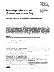
5.2.2. 5.2.2. Guide Guide Vane VaneBB ˝ The The next next stage stage proceeded proceeded by byfixing fixingthe theguide guidevane vaneatatββ==70 70°.. Seven Seven different different arrangements arrangements in in ˝ ˝ the range of ψ = 30 to 90 with 10 intervals were considered for guide vane B. Due to the range of ψ = 30° to 90° with 10 intervals were considered for guide vane B. Due to the the position position of of ˝ this this guide guide vane, vane, angles angles greater greaterthan than90 90°were were ignored. ignored. As As is is obvious obvious in in Figure Figure 17, 17, the the greatest greatest power power ˝ when it is equal to 0.134. coefficient belongs to the arrangement with ψ = 60 coefficient belongs to the arrangement with ψ = 60° when it is equal to 0.134.

Figure 17. 17. Effect Effect of of guide guide vane vane BB angle angle on on power power coefficient. coefficient. Figure

The results and other specifications of the tests are shown in Table 4. From this table it is The results and other specifications of the tests are shown in Table 4. From this table it is indicated indicated that ψ = 60° results in the highest power output with 3.49 W. The first column from the that ψ = 60˝ results in the highest power output with 3.49 W. The first column from the right shows right shows the relative deviations of the output power from the baseline design, when both β and ψ the relative deviations of the output power from the baseline design, when both β and ψ are equal to are equal to 90°, are also tabulated in Table 3. 90˝ , are also tabulated in Table 3. Table 4. The results and other specifications of the various cases.

A70B30 A70B40 A70B50 A70B60 A70B70 A70B80 A70B90

Cm

T

TSR

Cp

P

0.051 0.053 0.055 0.061 0.055 0.052 0.053

0.038 0.039 0.04 0.045 0.041 0.039 0.0392

2.2 2.2 2.2 2.2 2.2 2.2 2.2

0.114 0.117 0.121 0.134 0.122 0.1165 0.1168

2.96 3.04 3.15 3.49 3.19 3.02 3.03

Deviation from Baseline Design (%) 8.823529 11.76471 15.80882 28.30882 17.27941 11.02941 11.39706

Cm, coefficient of momentum; T, torque; TSR, tip speed ratio; Cp, coefficient of power; P, generated power.

The torque coefficient variation in two different arrangements for a complete revolution is compared in Figure 18. As it is clear, from θ = 0° to θ = 160°, both diagrams are relatively congruent;

Energies 2016, 9, 346

16 of 19

Table 4. The results and other specifications of the various cases.

A70B30 A70B40 A70B50 A70B60 A70B70 A70B80 A70B90

Cm

T

TSR

Cp

P

Deviation from Baseline Design (%)

0.051 0.053 0.055 0.061 0.055 0.052 0.053

0.038 0.039 0.04 0.045 0.041 0.039 0.0392

2.2 2.2 2.2 2.2 2.2 2.2 2.2

0.114 0.117 0.121 0.134 0.122 0.1165 0.1168

2.96 3.04 3.15 3.49 3.19 3.02 3.03

8.823529 11.76471 15.80882 28.30882 17.27941 11.02941 11.39706

Cm , coefficient of momentum; T, torque; TSR, tip speed ratio; Cp , coefficient of power; P, generated power.

The torque coefficient variation in two different arrangements for a complete revolution is compared in Figure 18. As it is clear, from θ = 0˝ to θ = 160˝ , both diagrams are relatively congruent; however, after this point the torque coefficient related to ψ = 60˝ is considerably higher until the end of the cycle, to a 15% higher average torque coefficient. Energies 2016, 9,leading 346 16 of 18

Figure 18. Torque coefficient coefficient of aa single single blade. blade.

6. Economic 6. EconomicFeasibility Feasibility A techno-economic techno-economic analysis analysis has has been been carried carried out out on on the the novel novel exhaust exhaust air air energy recovery wind wind A energy recovery turbine generator installed on a cooling tower commonly used in Malaysia. For the cooling tower turbine generator installed on a cooling tower commonly used in Malaysia. For the cooling tower with a 7.5rated kW rated fan motor, 13.3% ofdischarged the discharged energy is expected torecovered. be recovered. a year awith 7.5 kW fan motor, 13.3% of the energy is expected to be ForFor a year of of operation of the cooling tower with this system, approximately 7.3 MWh is estimated to be operation of the cooling tower with this system, approximately 7.3 MWh is estimated to be recovered. recovered.analysis Economic analysis shows that capital, components as well and as operation and Economic shows that capital, components replacement,replacement, as well as operation maintenance maintenance costs are of the system covered of inthe thesystem. lifetimeFor of this the system. For net thispresent project,(NPV) the net costs of the system covered in are the lifetime project, the is present (NPV) is 25,347 Malaysian Ringgit (RM) for the 20-year lifetime. 25,347 Malaysian Ringgit (RM) for the 20-year lifetime. 7. Conclusions Conclusions CFD study study was was carried carried out out on on aa novel novel wind wind turbine turbine design. design. The effects of different A 2D CFD diffuser plate angles and guide vane angles were investigated. It was derived from the results that by introducing diffusers and then guide vanes, the overall power output of the wind turbine was improved by respectively, compared to using a VAWT alone. In the by approximately approximately5% 5%and and34%, 34%, respectively, compared to using a VAWT alone. Incase the ˝ of theofdiffusers, the optimum angle angle was found to be 7°, guide and B, wasB,70° and case the diffusers, the optimum was found to while be 7 ,for while forvanes guideAvanes Aitand it was ˝ and 60°, respectively. These results in good with experimental results results obtained in the 70 60˝ , respectively. Theseare results are inagreement good agreement with experimental obtained laboratory. Overall, it can be concluded that exhaust air recovery turbines offer a promising in the laboratory. Overall, it can be concluded that exhaust air recovery turbines offer a technology. opportunity in green technology. Acknowledgments: The authors would like to acknowledge the Ministry of Higher Education of Malaysia and The University of Malaya, Kuala Lumpur, Malaysia for the financial support under Grant RP006C-13AET, HIRG: UM.C/HIR/MOHE/ENG/15 (D000015-16001), and Malaysia Technical Cooperation Program (MTCP) scholarship. Author Contributions: Seyedsaeed Tabatabaeikia, Behzad Shahizare, and Nima Izadyar have conceived CFD

Energies 2016, 9, 346

17 of 19

Acknowledgments: The authors would like to acknowledge the Ministry of Higher Education of Malaysia and The University of Malaya, Kuala Lumpur, Malaysia for the financial support under Grant RP006C-13AET, HIRG: UM.C/HIR/MOHE/ENG/15 (D000015-16001), and Malaysia Technical Cooperation Program (MTCP) scholarship. Author Contributions: Seyedsaeed Tabatabaeikia, Behzad Shahizare, and Nima Izadyar have conceived CFD simulation, performed experimental study and written this article. Nik Nazri Bin Nik-Ghazali and Wen Tong Chong are the heads of two groups in University of Malaya that guide all of the procedures. Ahmad Fazlizan and Alireza Esmaeilzadeh have assisted in paper writing and result analysis. Conflicts of Interest: The authors declare no conflict of interest.

Nomenclature A BEM CFD Ct, average Cp, average FT GIT k L R* P SST URANS U VAWT W Greek α β θ λ µ νeff ρ ψ ω

Swept turbine area Blade element momentum Computational fluid dynamics Average of mechanical torque coefficient Average power coefficient Tangential force Grid independency test Kinetic energy Turbulent length Monotonic divergence Dynamic pressure Shear stress transport Unsteady Reynolds averaged Navier-Stokes Air velocity Vertical axis wind turbine Relative velocity Diffuser angle Angle of guide-vane A Azimuth angle Tip speed ratio Viscosity Effective kinematic viscosity Density Angle of guide-vane B Angular velocity

References 1. 2. 3. 4.

5.

Manwell, J.F.; McGowan, J.G.; Rogers, A.L. Wind Energy Explained: Theory, Design and Application; John Wiley & Sons: Hoboken, NJ, USA, 2010. Energy Commission of Malaysia. Malaysia Energy Statistics Handbook 2014; Suruhanjaya Tenaga: Putrajaya, Malaysia. Available online: http://www.meih.st.gov.my (accessed on 24 May 2015). Sung, C.T.B. Possibility of electricity from wind energy in Malaysia: Some rough calculations. Available online: http://www.christopherteh.com/blog/2010/11/wind-energy/ (accessed on 24 May 2015). Chong, W.T.; Fazlizan, A.; Poh, S.C.; Pan, K.C.; Hew, W.P.; Hsiao, F.B. The design, simulation and testing of an urban vertical axis wind turbine with the omni-direction-guide-vane. Appl. Energy 2013, 112, 601–609. [CrossRef] Ohya, Y.; Karasudani, T. A shrouded wind turbine generating high output power with wind-lens technology. Energies 2010, 3, 634–649. [CrossRef]

Energies 2016, 9, 346

6.

7. 8. 9. 10. 11.

12.

13.

14. 15.

16. 17. 18. 19. 20. 21. 22.

23.

24. 25. 26. 27. 28.

18 of 19

Chong, W.T.; Pan, K.C.; Poh, S.C.; Fazlizan, A.; Oon, C.S.; Badarudin, A.; Nik-Ghazali, N. Performance investigation of a power augmented vertical axis wind turbine for urban high-rise application. Renew. Energy 2013, 51, 388–397. [CrossRef] Foreman, K.; Gilbert, B. Technical development of the Diffuser Augmented Wind Turbine/DAWT/concept. Wind Eng. 1979, 3, 153–166. Foreman, K.; Gilbert, B.; Oman, R. Diffuser augmentation of wind turbines. Solar Energy 1978, 20, 305–311. [CrossRef] Foreman, K. Preliminary Design and Economic Investigations of Diffuser-Augmented Wind Turbines (DAWT); Grumman Aerospace Corp.: Bethpage, NY, USA, 1981. Moeller, M.; Visser, K. Experimental and numerical studies of a high solidity, low tip speed ratio DAWT. In Proceedings of the 48th AIAA Aerospace Sciences Meeting and Exhibit, Orlando, FL, USA, 4–7 January 2010. Tong, C.W.; Chew, P.S.; Abdullah, A.F.; Sean, O.C.; Ching, T.C. Exhaust air and wind energy recovery system for clean energy generation. In Proceedings of the International Conference on Environment and Industrial Innovation, Kuala Lumpur, Malaysia, 4–5 June 2011; IACSIT Press: Kuala Lumpur, Malaysia, 2011. Shahizare, B.; Ghazali, N.N.B.N.; Chong, W.T.; Tabatabaeikia, S.; Izadyar, N. Investigation of the optimal omni-direction-guide-vane design for vertical axis wind turbines based on unsteady flow CFD simulation. Energies 2016, 9, 146. [CrossRef] Shahizare, B.; Nik-Ghazali, N.; Chong, W.; Tabatabaeikia, S.; Izadyar, N.; Esmaeilzadeh, A. Novel investigation of the different Omni-direction-guide-vane angles effects on the urban vertical axis wind turbine output power via three-dimensional numerical simulation. Energy Conv. Manag. 2016, 117, 206–217. [CrossRef] Mertens, S.; van Kuik, G.; van Bussel, G. Performance of an H-Darrieus in the skewed flow on a roof. J. Sol. Energy Eng. 2003, 125, 433–440. [CrossRef] Simms, D.A.; Schreck, S.; Hand, M.; Fingersh, L. NREL Unsteady Aerodynamics Experiment in the NASA-Ames Wind Tunnel: A Comparison of Predictions to Measurements; National Renewable Energy Laboratory: Golden, CO, USA, 2001. McTavish, S.; Feszty, D.; Sankar, T. Steady and rotating computational fluid dynamics simulations of a novel vertical axis wind turbine for small-scale power generation. Renew. Energy 2012, 41, 171–179. [CrossRef] McLaren, K.; Tullis, S.; Ziada, S. Computational fluid dynamics simulation of the aerodynamics of a high solidity, small-scale vertical axis wind turbine. Wind Energy 2012, 15, 349–361. [CrossRef] Edwards, J.M.; Danao, L.A.; Howell, R.J. Novel experimental power curve determination and computational methods for the performance analysis of vertical axis wind turbines. J. Sol. Energy Eng. 2012, 134. [CrossRef] Chowdhury, A.M.; Akimoto, H.; Hara, Y. Comparative CFD analysis of Vertical Axis Wind Turbine in upright and tilted configuration. Renew. Energy 2016, 85, 327–337. [CrossRef] Qin, N.; Howell, R.; Durrani, N.; Hamada, K.; Smith, T. Unsteady flow simulation and dynamic stall behaviour of vertical axis wind turbine blades. Wind Eng. 2011, 35, 511–528. [CrossRef] Castelli, M.R.; Englaro, A.; Benini, E. The Darrieus wind turbine: Proposal for a new performance prediction model based on CFD. Energy 2011, 36, 4919–4934. [CrossRef] Chong, W.T.; Hew, W.P.; Yip, S.Y.; Fazlizan, A.; Poh, S.C.; Tan, C.J.; Ong, H.C. The experimental study on the wind turbine’s guide-vanes and diffuser of an exhaust air energy recovery system integrated with the cooling tower. Energy Convers. Manag. 2014, 87, 145–155. [CrossRef] Chong, W.T.; Fazlizan, A.; Poh, S.C.; Pan, K.C.; Ping, H.W. Early development of an innovative building integrated wind, solar and rain water harvester for urban high rise application. Energy Build. 2012, 47, 201–207. [CrossRef] Fazlizan, A.; Chong, W.; Yip, S.; Hew, W.; Poh, S. Design and experimental analysis of an exhaust air energy recovery wind turbine generator. Energies 2015, 8, 6566–6584. [CrossRef] Paraschivoiu, I. Wind Turbine Design: With Emphasis on Darrieus Concept; Presses Inter Polytechnique: Montréal, QC, Canada, 2002. Fluent, A. 14.5 User’s Guide; Fluent Inc.: New York, NY, USA, 2012. Almohammadi, K.; Ingham, D.; Ma, L.; Pourkashanian, M. CFD sensitivity analysis of a straight-blade vertical axis wind turbine. Wind Eng. 2012, 36, 571–588. [CrossRef] Almohammadi, K.M.; Ingham, D.B.; Ma, L.; Pourkashan, M. Computational fluid dynamics (CFD) mesh independency techniques for a straight blade vertical axis wind turbine. Energy 2013, 58, 483–493. [CrossRef]

Energies 2016, 9, 346

29. 30. 31.

32. 33. 34. 35. 36.

19 of 19

Howell, R.; Qin, N.; Edwards, J.; Durrani, N. Wind tunnel and numerical study of a small vertical axis wind turbine. Renew. Energy 2010, 35, 412–422. [CrossRef] Yakhot, V.; Orszag, S.; Thangam, S.; Gatski, T.; Speziale, C. Development of turbulence models for shear flows by a double expansion technique. Phys. Fluids A Fluid Dyn. (1989–1993) 1992, 4, 1510–1520. [CrossRef] Chong, W.T.; Naghavi, M.S.; Poh, S.C.; Mahlia, T.M.I.; Pan, K.C. Techno-economic analysis of a wind-solar hybrid renewable energy system with rainwater collection feature for urban high-rise application. Appl. Energy 2011, 88, 4067–4077. [CrossRef] Lim, Y.C.; Chong, W.T.; Hsiao, F.B. Performance Investigation and Optimization of a Vertical Axis Wind Turbine with the Omni-Direction-Guide-Vane. Procedia Eng. 2013, 67, 59–69. [CrossRef] Schaffarczyk, A. Introduction to Wind Turbine Aerodynamics; Springer: Berlin, Germany, 2014. Lilley, G.; Rainbird, W. A Preliminary Report on the Design and Performance of Ducted Windmills; College of Aeronautics Cranfield: Cranfield, UK, 1956. Van Bussel, G.J. The science of making more torque from wind: Diffuser experiments and theory revisited. In Journal of Physics: Conference Series; IOP Publishing: Bristol, UK, 2007. Abe, K.; Nishida, M.; Sakurai, A.; Ohya, Y.; Kihara, H.; Wada, E.; Sato, K. Experimental and numerical investigations of flow fields behind a small wind turbine with a flanged diffuser. J. Wind Eng. Ind. Aerodyn. 2005, 93, 951–970. [CrossRef] © 2016 by the authors; licensee MDPI, Basel, Switzerland. This article is an open access article distributed under the terms and conditions of the Creative Commons Attribution (CC-BY) license (http://creativecommons.org/licenses/by/4.0/).