A Comparison between the Ensemble Kalman Filter and the Particle ...

A Comparative Study of the Particle Filter and the Ensemble Kalman Filter by

Syamantak Datta Gupta

A thesis presented to the University of Waterloo in fulfillment of the thesis requirement for the degree of Master of Applied Science in Electrical and Computer Engineering

Waterloo, Ontario, Canada, 2009

© Syamantak Datta Gupta 2009

I hereby declare that I am the sole author of this thesis. This is a true copy of the thesis, including any required final revisions, as accepted by my examiners. I understand that my thesis may be made electronically available to the public.

ii

Abstract Non-linear Bayesian estimation, or estimation of the state of a non-linear stochastic system from a set of indirect noisy measurements is a problem encountered in several fields of science. The particle filter and the ensemble Kalman filter are both used to get sub-optimal solutions of Bayesian inference problems, particularly for high-dimensional non-Gaussian and non-linear models. Both are essentially Monte Carlo techniques that compute their results using a set of estimated trajectories of the variable to be monitored. It has been shown that in a linear and Gaussian environment, solutions obtained from both these filters converge to the optimal solution obtained by the Kalman Filter. However, it is of interest to explore how the two filters compare to each other in basic methodology and construction, especially due to the similarity between them. In this work, we take up a specific problem of Bayesian inference in a restricted framework and compare analytically the results obtained from the particle filter and the ensemble Kalman filter. We show that for the chosen model, under certain assumptions, the two filters become methodologically analogous as the sample size goes to infinity.

iii

Acknowledgements First and foremost, I would like to thank sincerely my supervisor Professor Ravi R. Mazumdar for his support, encouragement and guidance. Working under his supervision has been a great learning opportunity for me. His encouragement has helped me learn a lot and has also induced in me a desire to learn more. Interactions with him has not only helped me expand my academic horizons, but has helped on a personal level as well. It has truly been s privilege to be his student. I would also like to express my sincere gratitude to Professor Patrick Mitran, whose course, Statistical Signal Processing provided a great deal of background knowledge for my research. Finally, I would like to thank my parents, who have encouraged and motivated me greatly and without whose love, care and support, it would have been impossible for me to be where I am today.

iv

Contents List of Tables

vii

List of Figures

viii

1 Introduction

1

1.1

Background . . . . . . . . . . . . . . . . . . . . . . . . . . . . . . .

1

1.2

The Optimum Solution . . . . . . . . . . . . . . . . . . . . . . . . .

1

1.3

Sub-optimal Approaches . . . . . . . . . . . . . . . . . . . . . . . .

2

1.4

Monte Carlo Methods

. . . . . . . . . . . . . . . . . . . . . . . . .

3

1.5

Problem Description . . . . . . . . . . . . . . . . . . . . . . . . . .

4

2 Related Work

6

2.1

Convergence Results for the Particle Filter . . . . . . . . . . . . . .

6

2.2

Convergence Results for the Ensemble Kalman Filter . . . . . . . .

8

2.3

Experimental Comparisons of the Two Methods . . . . . . . . . . .

8

3 Analytical Approach to the Problem

10

3.1

A Generalized Problem Formulation . . . . . . . . . . . . . . . . . .

10

3.2

The Analytical Approach . . . . . . . . . . . . . . . . . . . . . . . .

11

3.3

A More Specific Model . . . . . . . . . . . . . . . . . . . . . . . . .

13

4 The Particle Filter

15

4.1

Introduction . . . . . . . . . . . . . . . . . . . . . . . . . . . . . . .

15

4.2

Description of the Algorithm . . . . . . . . . . . . . . . . . . . . . .

16

4.3

Choices of Proposal Distribution and Importance Weights

. . . . .

17

4.4

Parameters for the Specified Model . . . . . . . . . . . . . . . . . .

18

4.5

Resampling . . . . . . . . . . . . . . . . . . . . . . . . . . . . . . .

19

v

5 The Ensemble Kalman Filter

22

5.1

The Discrete Kalman Filter . . . . . . . . . . . . . . . . . . . . . .

23

5.2

The Ensemble Kalman Filter Algorithm . . . . . . . . . . . . . . .

24

6 An Analytical Comparison of the Two Schemes

28

6.1

Introduction . . . . . . . . . . . . . . . . . . . . . . . . . . . . . . .

28

6.2

Convergence Results for the Ensemble Kalman Filter Estimates . .

29

6.3

A Relation between the Expectations of the Solutions of the Two Methods . . . . . . . . . . . . . . . . . . . . . . . . . . . . . . . . .

34

A Relation between the Covariances of the Solutions of the Two Methods . . . . . . . . . . . . . . . . . . . . . . . . . . . . . . . . .

36

General Remarks . . . . . . . . . . . . . . . . . . . . . . . . . . . .

38

6.4 6.5

7 Simulation Results

40

8 Conclusion and Future Work

51

APPENDIX

55

References

60

vi

List of Tables 7.1

Average estimation errors for the particle filter and the ensemble Kalman filter for different sample sizes . . . . . . . . . . . . . . . .

vii

50

List of Figures 4.1

Flow chart illustrating particle filter algorithm . . . . . . . . . . . .

21

5.1

Flow chart illustrating ensemble Kalman filter algorithm . . . . . .

27

7.1

Ns = 5, error versus time plot for particle filter . . . . . . . . . . .

41

7.2

Ns = 5, error versus time plot for ensemble Kalman filter . . . . . .

42

7.3


42

7.4

Ns = 20, error versus time plot for ensemble Kalman filter . . . . .

43

7.5


43

7.6


44

7.7

Ns = 100, error versus time plot for particle filter . . . . . . . . . .

44

7.8


45

7.9

Ns = 5, average error versus time plot for particle filter . . . . . . .

46

7.10 Ns = 5, average error versus time plot for ensemble Kalman filter .

46

7.11 Ns = 20, average error versus time plot for particle filter . . . . . .

47


47


48


48


49

7.16 Ns = 100, average error versus time plot for ensemble Kalman filter

49

viii

Chapter 1 Introduction 1.1

Background

Estimation of the state of a stochastic system from indirect noisy measurements is a problem encountered in several fields of science. These include a diverse class of problems in econometrics, biostatistics, geology and meteorology as well as many typical statistical signal processing problems such as target tracking, time series analysis, communications and satellite navigation. In all these problems, one essentially has the task of accurately estimating a certain set of variables that evolve over time, from a set of noisy measurements. Such a problem comes under the category of Bayesian inference problems, a sub-class of statistical inference where the likelihood of a hypothesis is updated sequentially in the light of observed data. Many such problems are formulated as discrete time hidden Markov models, where it is assumed that the present state of the system depends only on the state at the preceding instant. The evolution of the state variables and their mathematical relation with the observed data may be known or may be hypothesized based on experience. Either ways, the model connecting the observations and the variables of interest is in general a probabilistic one, due to the presence of noise and/or other uncertainties; and as such there is a need to determine a scheme that would lead to an optimum or sub-optimal solution.

1.2

The Optimum Solution

When the dynamics of this model are entirely linear and the noises involved are additive, following Gaussian distributions with known parameters, the optimum solution is given by the Kalman filter (Kalman [1960]). The discrete Kalman filter is a very robust and useful tool that has found its application in a wide variety 1

of problems encountered in various fields of science and technology, and is based on minimizing the estimation errors. However, a linear and Gaussian environment accounts for a very small subset of Bayesian inference problems; in most cases the system dynamics are non-linear and the noises non-Gaussian. In such situations analytical solutions are often intractable. Higher dimensionality of the system also adds to the complexity of the problem. Even for linear and Gaussian models, the Kalman filter may not be a feasible scheme to apply when the state dimensions are too high. For instance, if the state dimension is N = 106 , then execution of the Kalman filter involves storage of an N × N matrix that would occupy a huge amount of memory.

1.3

Sub-optimal Approaches

Among these, the extended Kalman filter (Maskell and Gordon [2001]) can be utilised when the problem involves one or more non-linear function. Essentially, it linearizes the non-linear function locally at several regions using the first term of its Taylor series expansion. Some versions of this filter also use a few higher order terms of the expansion, but these are not used extensively for the obvious rise in computational complexity. The method assumes the noises to be Gaussian and uses the equations of the discrete Kalman filter to obtain the final estimate at each step of estimation. Because it assumes a Gaussian environment, this method would not work well when the distributions are significantly non-Gaussian. Moreover, it does not give good results under severe non-linearity, because then the local linearisations do not emulate well enough the original function. While the extended Kalman filter attempts to emulate an optimal solution by linearizing the non-linear functions, the approximate grid-based methods attempt the same by discretising a continuous state space. In the latter, the continuous state domain is divided into a finite number of states around certain points within the domain and probability density functions involved in the estimation are reduced to probability mass functions. Prediction and update equations are formed using the conditional probabilities of each state with respect to the observations. For this model to approximate closely the actual dynamics of the state variable, in general, the discrete grid must be dense enough. It is intuitive that if the original space is known beforehand to be sparse, and the regions of high occurrence are known too, this method can be useful. However, in most cases one has no a priori knowledge of the distribution of the state space, and hence it is not possible to partition it unevenly by assigning greater resolution to the regions of greater likelihood. Another disadvantage of this method is the inevitable truncation of certain portions of the state space. 2

1.4

Monte Carlo Methods

The ensemble Kalman filter and the particle filter both are essentially Monte Carlo estimation methods and work on the following basic principle. First, a domain of possible input points is defined. For Bayesian estimation problems, this is equivalent to defining the a priori probability distribution. Next, a fixed number of sample points are generated from this domain or distribution. Using these sample points, finally, the required variables or parameters are estimated by performing a numerical integration. It is intuitively evident, therefore, that these methods rely on the law of large numbers, as they tend to replace integrations involving probability terms with deterministically computed sums and averages, effectively approximating probability with relative frequency of occurrence when the sample size is sufficiently large. The fact that Monte Carlo methods such as the ones mentioned above can be used to solve complicated integrals numerically was known for a considerable time. However, the implementation of these methods for practical computational purposes was not feasible until recently. Over the recent years, thanks to advances in the fields of computing there has been an increased interest and popularity in these techniques. Monte Carlo methods are widely applied to a variety of problems in several fields of science. Many of these problems involve simulation of a physical system, many other involve prediction and estimation of unknown variables. The particle filter and the ensemble Kalman filter are both extensively used to get sub-optimal solutions of Bayesian inference problems, particularly in case of highdimensional non-Gaussian and non-linear models. The particle filter (Moral [1996]) is a recursive filtering method that generates multiple copies of the variable of interest from a sample population, associates a specific weight to each of these copies and then computes their weighted average to get the final estimate. Samples for the unknown states are drawn from an approximate distribution, and the optimal estimate is obtained by taking a weighted average of the samples, where the weights are assigned using the principle of importance sampling. This method has been called bootstrap filtering, sequential Monte Carlo method, the condensation algorithm, interacting particle approximation and survival of the fittest by different authors and researchers (Maskell and Gordon [2001]). The Monte Carlo characterisations tend to approach the original distribution as the sample size becomes sufficiently large, and the filter approaches the optimal Bayesian estimate. Simply put, this technique draws samples for the state variable from a dummy distribution q(·) in lieu of the original distribution p(·) as sampling from the latter directly may not be feasible. The dummy distribution, also known as the proposal distribution q(·) is related to the original distribution in terms of importance 3

weights. Finally the required estimate is computed by combining the sample points drawn from q(·) with the corresponding importance weights. At each point, the state estimates are being developed simultaneously from each realisation of the sample along separate trajectories. The use of importance weights basically ensure that trajectories that more closely emulate the observations are assigned greater importances. The ensemble Kalman filter (Evensen [1994]), on the other hand is an approximate extension of the discrete Kalman Filter used for non-linear Bayesian filtering. This method involves generating ensembles of model states and arriving at the final result using those samples and the observed measurements. An ensemble of forecast estimates is predicted here based on the estimates at the previous instant, and then those forecasts are tuned using an ensemble Kalman gain once the most recent observations arrive. It may be noted that the ensemble Kalman filter works best under Gaussian environments and do not give desired results when the probability distribution of the relevant variable deviates significantly from the Gaussian distribution. It has been shown that under a linear and Gaussian environment, solutions obtained from both these filters converge to the optimal solution obtained by the Kalman Filter (Mandel et al. [2009], Butala et al. [2008], Saygin [2004]). Several convergence results for the particle filter under different conditions have also been derived and analyzed. Issues such as the asymptotic convergence of the filter solution to the optimal solution, error accumulation with time, convergence of the mean square error and convergence of the empirical distributions to the true ones have been addressed (Crisan and Doucet [2002]). Given the similar natures of the two filtering mechanisms, it would be an interesting problem to explore how they compare and relate to each other in basic methodology and construction.

1.5

Problem Description

In this work, we would take up a specific problem of Bayesian inference in a restricted framework. Namely, the noises involved are assumed to be zero-mean Gaussian with known covariance matrices, and the observations are linearly related to the states. For a model of this kind, an analytical comparison of the results obtained from the particle filter and the ensemble Kalman filter would be done. It would be shown that for the given model, the two methods closely resemble each other in their approaches, though they differ in their ultimate results. More specifically, it would be shown that when the sample size is sufficiently large, the two filters essentially follow the same procedure to create estimate trajectories. However, even when the sample size is significantly large, the particle 4

filter, because it ascribes greater importance weights to trajectories that are more likely to produce the observed measurements, is, in general, more likely to give more accurate results. The basic problem being considered is the determination or prediction of a parameter θ that changes over some variable, usually time, using a series of noisy observations x. The parameter of interest θ is generally assumed to evolve over time following some known probabilistic model, depending on its previous state(s) and external disturbances. The observed variable x is some function of θ , contaminated with some noise. Let us now enumerate the contents of this work. A discrete time formulation of the problem would be considered, where state evolution and availability of measurement both are assumed to occur at the same instants. Starting from a general description of the problem we would narrow our attention to a special case. We would then look at the development of a general Bayesian filtering approach, applicable to both linear and non-linear models; and show how such an analytical method would fail to provide a direct solution in many cases because of the integrals that it involve. Then, we would take up separately the two methods of interest in this study, discuss their working principles and formulate the structure of the solutions given by them. Here, we would attempt to solve a standard problem of Bayesian inference in case of a Gaussian system where the observations are linearly related to the parameter of interest but the state evolution dynamics of the parameter itself are non-linear. We would then study how the two solutions relate to each other. We would establish, under certain assumptions, an analytical relation between the set of solutions provided by the two methods and show that as the ensemble size goes to infinity, the ensemble Kalman filter trajectories approximate the particle filter trajectories. The general similarity would also be demonstrated through simulation. Finally, we would briefly discuss the implications of this results and the future directions of work in this regard.

5

Chapter 2 Related Work As seen in the previous chapter, except for a very limited scenario, it is not easy to estimate the optimum solutions for the states of a stochastic process directly from a set of noisy observations. Subsequently, several sub-optimal approximate methods have been derived over the years. The fact that solutions for high-dimensional nonlinear state estimation problems can be derived by manipulating a large number of sample points was well known from a theoretical perspective, and with the recent advances in computing abilities, such methods have begun to gain popularity in a wide range of practical fields. The particle filter and the ensemble Kalman filter are both sequential Monte Carlo methods that estimate the state variables using a large number of sampled data points. A detailed and rigorous mathematical formulation of the particle filter can be found in Moral [1996] where the technique is elaborately explained starting from the first principles, while Doucet et al. [2000], too, provides a comprehensive study. Ensemble Kalman filters, on the other hand were introduced as an approximation of the Kalman filter in Evensen [1994]. Several convergence results have been derived for the particle filter, and some for the ensemble Kalman filter. However, analytical comparisons between the two filters with an aim to establish a correlation between the two do not seem to have been abundant.

2.1

Convergence Results for the Particle Filter

A thorough discussion on the convergence results for the particle filter is available in Crisan and Doucet [2002]. After providing a detailed mathematical framework for the filter, this paper explores some results on almost sure convergence, convergence of the mean square error and a large deviations result. Specifically, it has been shown that under the assumption that the transition Markov kernel is Feller, and 6

that the likelihood function (this is the conditional probability density function of the observed variables given the state variables) is bounded, continuous and strictly positive, the empirical distribution obtained from the particle filter converges almost surely to the true distribution of the state. Further, it shows that convergence of the mean square error towards zero is guaranteed and it occurs with a rate in 1/N when a standard resampling scheme is used and the importance weights are upper bounded. Another result presented in this work implies that a uniform convergence of the particle filter is ensured if the ‘true’ optimal filter is quickly mixing, while a considerable amount of error accumulation will prevent such a convergence when the optimal filter has a ‘long memory’. This indicates that for Markov processes, one would expect a uniform convergence. Again, in a fairly recent work, Hu et al. [2008], it has been shown that the approximate solution given by the particle filter converges to the true optimal estimate, even when the function to be estimated is unbounded, as the sample size goes to infinity. In a recent study (Bengtsson et al. [2008]) that analytically explores the performance of sequential Monte Carlo based methods, and the particle filter in particular, it has been shown that for models with high dimensions, the sequential importance sampling method tends to collapse to a single point mass within a few cycles of observation. The paper provides general conditions under which the maximum of the importance weights associated with the individual trajectories of the particle filter approaches unity, if the particle size is sub-exponential in the cube root of the system dimension. The convergence result is derived for a Gaussian setting, but it has been argued that the result would also hold for observation models with any other independent and identically distributed (iid) kernel. The study also asserts that even though methods such as resampling may be employed as a remedy to this degeneracy phenomenon for small scale models, they would not be able to eliminate the problem of slow convergence rates for systems with large dimensions. In Saygin [2004] it has been shown that for the linear Gaussian state model, the optimal solution given by the interactive particle systems converges asymptotically to the real predictor conditional density given by the optimal Kalman Filter. The proof is first given for a uni-dimensional model and is then extended for the multidimensional case. Further, this work has explored how large the sample size is required to be for the filter to follow this asymptotic behaviour.

7

2.2

Convergence Results for the Ensemble Kalman Filter

Though the ensemble Kalman filter has not yet been as rigorously analyzed as its counterpart, some recent works have studied the nature of its convergence under certain restricted conditions. In Furrer and Bengtsson [2007], it has been mentioned that an asymptotic convergence of the ensemble Kalman filter can be shown using Slutsky’s theorem, without providing a rigorous proof. Butala et al. [2008] provides a more convincing result by showing that as the size of the ensemble grows exponentially, the ensemble Kalman filter estimates converge in probability to LMMSE optimal estimates obtained by the Kalman Filter for a linear and Gaussian model. This work also provides a formal argument for the proposition that the ensemble Kalman filter is a Monte Carlo method that converges to a well defined limit. In another recent work (Mandel et al. [2009]), it has been shown that the filter converges to the discrete Kalman filter as the ensemble size goes to infinity for a linear and Gaussian model and constant state space dimension. This work has first proved that the ensemble members are exchangeable random variables bounded in Lp and has then used this result, Slutsky’s theorem and the Weak Law of Large Numbers to establish their final conclusion. Since the ensemble Kalman filter approximates covariance terms by averaging over a large number of data points, it is expected to give better results as the ensemble size increases. This has been demonstrated in Gillijns et al. [2006], where simulation results show a steady fall in estimation errors as the ensemble size grows.

2.3

Experimental Comparisons of the Two Methods

Some studies have examined and compared the performances of the two filtering methods in a real experiment. In these experiments, in general, the particle filter has been seen to outperform its counterpart in terms of accuracy, because of its more sound mathematical foundations and also because of the fact that it makes lesser assumptions about the nature of the distribution to be estimated. The ensemble Kalman filter implicitly assumes the distribution to be Gaussian by relying only on the first two moments for estimation, and this makes it unreliable when the system dynamics are significantly non-Gaussian. In Nakamura et al. [2009], the authors explore the merits of the two filters with respect to each other for data assimilation and tsunami simulation models. The models used are Gaussian and non-linear; and experimental results show that the 8

particle filter outperforms its rival quite convincingly in terms of accurate estimation. In some of the practical applications though, a choice between the two filters involve a trade-off between accuracy and computational burden; and the ensemble Kalman filter may in fact be preferred because it is relatively simpler in formulation and also because it might involve less computational burden. The work Weerts and El Serafy [2006], for instance, has taken up the task of comparing the performances of several non-linear filters (and in particular the two filters in our study), in the context of flood prediction, a key issue in hydrology. This paper suggests that since the particle filter utilises the full prior density, without making assumptions on the prior distribution of the model states, as opposed to the ensemble Kalman filter, it has a greater sensitivity towards the tails of the distribution and this makes it extremely advantageous in flood forecasting. However, this advantage is achieved at the cost of higher computational complexities. Also, it is said that the particle filter is more affected by error in measurement or system modeling, while the ensemble Kalman filter is more robust in that respect. It is thus stated that the ensemble Kalman filter appears to be more efficient than the particle filter for low flows, because of its relatively lesser susceptibility to uncertainties and misspecification of model parameters. The theoretical studies imply that both the models would give optimal solutions under certain restricted conditions, as the sample size or ensemble size goes to infinity. The experimental studies indicate that even though the particle filter is theoretically superior, in some practical applications the ensemble Kalman filter may in fact be preferred to reduce computational burden. Since both the filters are used to solve similar estimation problems and also use similar techniques, it is of interest to explore how the schemes relate to each other from an analytical perspective. With this motivation, let us now proceed to describe the details of the actual problem that would be approached.

9

Chapter 3 Analytical Approach to the Problem 3.1

A Generalized Problem Formulation

Having briefly discussed the objectives of this study, let us now first describe the problem in details. Subsequently we would formulate the steps of a general solution. As mentioned before, the problem that we are concerned with is to estimate states of a hidden Markov chain from a set of noisy observations. For the ease of construction, a discrete time formulation is being considered, where the state evolution occurs at fixed instants, and these are the same instants when measured observations are made available. Clearly, since we have two sets of variables in this problem, of which one, viz., the state vector, evolves over time and the other, viz., the set of measurements, changes accordingly, we would require two mathematical models, or two sets of equations to describe the system. One of them would describe the evolution of the state with time while the other would relate the measured data with the present state. For the most general case, these two sets of equations would have the following forms. The state evolution of the parameter of interest θt would be described by the following hidden Markov model: θt+1 = ft (θt , wt ) ∀ t ∈ N

(3.1)

The observations would be related to the state variables as per the following equations: xt = ht (θt , vt ) ∀ t ∈ N 10

(3.2)

where ft : RNθ × RNw → RNθ and ht : RNθ × RNv → RNx are any functions, possibly non-linear.

3.2

The Analytical Approach

Let us now proceed to construct an analytical solution of this inference problem. Since both the state evolution and the observations are mixed with unknown disturbances in the form of random noise, and hence are probabilistic, it is useful to consider probabilistic models for estimation. The general framework of methods that solve such problems is typically based on the Bayesian approach. The aim is to determine the posterior probability density function (pdf) of the state using all the information available from past history of the state and the measured data (Maskell and Gordon [2001]). Given the transition equation (which, in our case is equation (3.1)) that describes the evolution of a hidden Markov process {θt ; t ∈ N}, an observation equation (which, in this case is equation (3.2)) that describes the conditional likelihood of the observations given the process, and the sequence of observations {xt ; t ∈ N} over t; this method attempts to find a best estimate of the conditional probability p(θ1 , θ2 , . . . , θt |xt , x2 , . . . , xt ) (denoted by p(θ1:t |x1:t )). Often the requirement is to only obtain the optimal estimate for the present instant and not the entire path of trajectory; in which case we attempt to obtain the conditional distribution of the variable at the present instant only. Instead of determining p(θ1:t |x1:t ), then, we only need to find out p(θt |x1:t ). Since the measurement needs to be updated every time a new data entry is received, a recursive filter would be convenient for the purpose. Once this probability is obtained, estimation of any function g(·) of θt can be done (provided g(θ1:t )p(θ1:t |x1:t ) is integrable); a very special (yet common) example is where g(α) = α, in which case the requirement would be the estimation of θt itself. In these kind of estimation problems, the initial conditional pdf p(θ0 |x0 ) is either known or is assigned an a priori value. Depending on the nature of the functions involved, this initialisation may or may not influence the convergence of the filter significantly. Such a filter has two stages: prediction and update. In the prediction stage, the state pdf at some instant t is forecasted based on all the prior information up to the instant t − 1 . In the update stage, this forecasted estimate is tuned and modified using the latest measurements for the instant t. Let us suppose that up to the instant t − 1, t ∈ N, the pdf p(θt−1 |x1:t−1 ) is available, i.e., it is either known or has been estimated. Because of the Markov property of the process, we also have p(θt |θt−1 , x1:t−1 ) = p(θt |θt−1 ), i.e., the distribution at the present instant depends only on the distribution at the previous instant and is independent of distributions at any instant prior to the last instant. 11

At the prediction stage, then, the posterior for the next instant can be predicted as follows.

Z p(θt |x1:t−1 ) =

p(θt ∩ θt−1 |x1:t−1 )dθt−1

p(θt ∩ θt−1 ∩ x1:t−1 ) dθt−1 p(x1:t−1 ) Z p(θt |θt−1 , x1:t−1 )p(θt−1 ∩ x1:t−1 ) = dθt−1 p(x1:t−1 ) Z p(θt−1 ∩ x1:t−1 ) dθt−1 = p(θt |θt−1 , x1:t−1 ) p(x1:t−1 ) Z = p(θt |θt−1 , x1:t−1 )p(θt−1 |x1:t−1 )dθt−1 Z

=

(3.3)

Using the fact the θt is Markovian, and hence depend only on θt−1 , we get Z p(θt |x1:t−1 ) =

p(θt |θt−1 )p(θt−1 |x1:t−1 )dθt−1

(3.4)

At each step, the integration is over the entire domain of θt−1 which is in fact the domain of θt , in general, for all t. In the next stage, once measured data for the current instant arrive, the above prediction (or the prior) is modified to obtain the optimal posterior density, using Bayes’ rule. p(θt |x1:t ) =

p(xt |θt )p(θt |x1:t−1 ) p(xt |x1:t−1 )

(3.5)

where the denominator is a normalizing constant, given by the Chapman-Kolmogorov equation as follows. Z p(xt |x1:t−1 ) =

p(xt |θt )p(θt |x1:t )dθt

(3.6)

In the above sets of equations, p(θt |θt−1 ) is the state transition probability distribution for θt while p(xt |θt ) is the conditional probability of xt given θt . Ideally, both these probabilities should be available when the functions involved and noise distributions are known and hence the solution of the problem may appear to be straightforward at a glance. However, even when the functions are known, in general, the integrals involved in (3.4) and (3.6) cannot be determined analytically, except for a few special cases. For instance, an optimum solution can be derived when the functions are linear and the noises are additive and Gaussian. As one 12

would expect, the solution derived under this specific model is the same as that obtained by the Kalman filter. For most cases though, a direct solution is either not feasible or not tractable and one has to depend on approximate methods for sub-optimal solutions. In fact, the above set of recursive equations only gives a conceptual framework of the solution.

3.3

A More Specific Model

So far we have described the problem from a general point of view where both the functions ft , ht may be non-linear, the noises may not be additive and they may not be Gaussian either. Let us now describe the special case of this problem which we are about to explore. It is assumed that the state evolution follows a known non-linear function while the observations are linearly related to the present states. We thus replace the non-linear function ht (·) with a matrix Ht . Noises involved at state evolution and observations are assumed to additive and zero-mean Gaussian with known covariance matrices. Under these conditions the parameter of interest θt is modeled as a discrete-time non-linear system with the following dynamics: θt+1 = f (θt ) + wt ∀ t ∈ N

(3.7)

The observations are described by the following equations: xt = Ht θt + vt ∀ t ∈ N

(3.8)

where, θt is the realisation of the unknown parameter θ at the instant t ∈ N, and xt is the observation vector at each instant t. We assume that the noises wt , vt are i.i.d. and follow Gaussian distributions with mean zero and known covariance matrices Qt , Rt respectively. The function f (θt ) that determines evolution of the state is known and defined for t > 0. It is also assumed that θt , wt and vt are uncorrelated. The state variable θt and the observation xt are both vectors with finite dimensions N and M respectively and in general, N > M . Then, wt and vt are vectors of dimensions N and M respectively; Ht is a real matrix of dimension M × N ; and Qt , Rt are N × N and M × M square matrices. Evidently, for the specific problem we are interested in, p(θt |θt−1 ) is the pdf of a Normal Distribution with mean f (θt−1 ) and covariance matrix Qt ; while p(xt |θt ) is the density of a Normal distribution with mean Ht θt and covariance matrix Rt . 13

This means that for this problem, the integral in 3.4 would also involve the nonlinear function f (·), and depending on its nature it may or may not be tractable.

14

Chapter 4 The Particle Filter 4.1

Introduction

A Particle filter (Moral [1996], Doucet et al. [2000], Maskell and Gordon [2001]) is essentially a sequential Monte Carlo estimation technique that is used for solving a wide variety of problems involving non-linearity and high dimensionality. In different papers and works, different terms have been used to describe this filtering mechanism. These names include bootstrap filtering, sequential Monte Carlo method, the condensation algorithm, interacting particle approximation and survival of the fittest. There are some minor differences in the different versions of the particle filter that are in use, and some algorithms use additional steps that are not employed by others, but fundamentally they are all based on the same basic principle. The method uses a set of point mass random samples (called ‘particles’) of probability densities and constructs a representation of the posterior density function by combining them, using a set of so-called ‘importance weights’. There are several variants of the particle filter which can be broadly categorized into two groups (Haug [2005]). In one, the same particles are re-used as trajectories while in the other particles are not re-used and fresh particles are generated at each step. Since our aim is to do a comparison of the particle filter with the ensemble Kalman filter, we have chosen to consider the filter that comes to the first category because of its intuitive similarity to the ensemble Kalman filter. Moreover, this model, known as the sequential importance sampling (SIS) particle filter is also more popular compared to its counterpart. In this scheme, starting from the same initial conditions, several dynamic realisations or trajectories of the state are developed over time, using the available information from past and present. The optimal solution at each step is a weighted average of all these different trajectories. The weights attached to the different paths of realisation indicate the relative likelihood of the corresponding trajectory. 15

As the number of samples increase, the solution of this filter approaches the optimal Bayesian estimate. To further facilitate the procedure, an additional step is included, which is known as resampling. This is done to eliminate the effects of filter degeneracy, or the situation when only a few of the trajectories being computed have a weight large enough to contribute to the final solution, while the weights associated with the rest are too insignificant to have any prominence. Under such conditions, particles are resampled and the optimum estimate is computed using modified weights.

4.2

Description of the Algorithm

The basic steps involved in the particle filter algorithm are now described (Maskell and Gordon [2001]). Let {θˆti ; t ∈ N, i = 1(1)Ns } be a set of samples of size Ns drawn from a distribution that is an approximate representation of the posterior. Let ωti be the respective weights associated with the sample points. By definition, initial points θˆ0i = θ0 for all i. The posterior density at an instant t can then be estimated as:

p(θ0:t |x1:t ) ≈

Ns X

i ωti δ(θ0:t − θˆ0:t )

(4.1)

i=1

where the weights are normalized, i.e., Ns X

ωti = 1

(4.2)

i=1

It follows that the estimates for θt over time are given by a weighted sum of the individual particle trajectories, where the weights are defined in equations (4.1) and (4.2).

θˆ0:t,P F |x1:t =

Ns X

i ωti θˆ0:t

(4.3)

i=1

When only an estimate at the present instant t is of interest, the above reduces to

θˆt,P F |x1:t =

Ns X i=1

16

ωti θˆti

(4.4)

It is evident, then, that this method consists of two major steps, viz., selection of a suitable distribution to draw samples for θˆti , and assignment of proper weights ωti to those samples. An ideal distribution to draw samples from would be the posterior itself, but that is impossible in most cases. As such, a method called Importance Sampling is employed. Here one requires to identify a proposal density q(·) from which samples can be drawn easily. The true weights, then are evaluated from the following equations : ωti∗ =

i p(θˆ0:t |x1:t ) i q(θˆ0:t |x1:t )

(4.5)

and, after normalizing, ωti

ωti∗

= PNs

i=1

ωti∗

(4.6)

When the proposal distribution q(·) satisfies the following properties, q(θ0:t |x1:t ) = q(θt |θ0:t−1 , x1:t )q(θ0:t−1 |x1:t−1 )

(4.7)

q(θt |θ0:t−1 , x1:t ) = q(θt |θt−1 , xt )

(4.8)

the importance weights can be shown to follow a simple recursive relation as follows: i ωti ∝ ωt−1

i p(xt |θti )p(θˆti |θˆt−1 ) i q(θˆti |θˆt−1 , xt )

(4.9)

The estimate equation for the posterior then reduces to

p(θt |x1:t ) ≈

Ns X

ωti δ(θt − θˆti )

(4.10)

i=1

4.3

Choices of Proposal Distribution and Importance Weights

Critical in this method are the choices of the proposal distribution q(·) and those of the importance weights ωti . As is apparent from the discussion so far, choice of the proposal q(·) plays a crucial role in this methodology during the sampling stage, 17

while a good choice of importance weights becomes important while combining the samples to get the best estimate. A good choice is to select that q(θt |θt−1 ) which i minimizes the variance of real weights ωti∗ , given θˆt−1 and xt . Such a choice maximizes the effective sample size Ns,ef f ; thereby reducing the effects of degeneracy of the filter. The optimal importance density function based on this consideration can be shown to be

i i p(xt |θt , θˆt−1 )p(θt |θˆt−1 ) i i q(θt |θˆt−1 , xt )optimal = p(θt |θˆt−1 , xk ) = i p(xt |θˆt−1 )

(4.11)

Under these conditions, the weights given by (4.9) become: i i ωti ∝ ωt−1 p(xt |θˆt−1 )

(4.12)

The above gives a general framework for the operation of the particle filter. It may be noted that the model described thus far is one among several variants of the so-called particle filter and these variants have minor differences in their operating principles. To obtain the optimal importance density it is required to draw samples from i p(θt |θˆt−1 , xk ) and subsequently evaluate an integral; which may not be straightforward in many cases, depending on the dynamics of the system. There are special cases, however, where the integration may be analytically feasible. The model used in this discussion, which assumes the noises to be i.i.d. Gaussian and the relation between the observed data and the system parameters to be linear, is one such example where the integration is not intractable and the parameters of the required distributions can be easily determined.

4.4

Parameters for the Specified Model

Referring to the model described by (3.7) and (3.8), we can then construct the following conditional probabilities (Doucet et al. [2000]): i p(θˆti |θˆt−1 , xt ) = N (θˆti ; µit , ψt )

(4.13)

T −1 T −1 −1 −1 î µit = (Q−1 t−1 + Ht Rt Ht ) (Qt−1 f (θt−1 ) + Ht Rt xt )

(4.14)

where

18

−1 T (ψt )−1 = Q−1 t−1 + Ht Rt Ht ∀ i = 1(1)Ns

(4.15)

where Ns is the sample size. The importance weights of the different trajectories ωti would be recursively obtained using the following conditional probability in equation (4.12). i i ), Rt + Ht Qt−1 HtT ) ) = N (xt ; Ht f (θˆt−1 p(xt |θˆt−1

(4.16)

where N (a; µ, ψ) denotes the probability density function of a vector a that follows a Normal distribution with mean µ and covariance matrix ψ. For the recursive equations described by (4.12) we would start with an initialisation of equal weights for each trajectory, meaning that all the realisations are considered equally important at the initial stage. At the subsequent steps, the importance weights would be modified according to (4.16), which would assign greater importance to trajectories that are more likely to generate the recorded observations. The optimal solution for θˆt at any instant t would be its conditional expectation computed using the probability given by (4.4).

4.5

Resampling

An additional step introduced in this particular algorithm is resampling. This is performed to reduce the effects of filter degeneracy. Degeneracy is the situation that arises when only a few of the sampled trajectories contribute to the final computed values by means of their higher weights, while others play a very insignificant role in the estimation as their corresponding weights are exceedingly small. Such a situation would ruin the main purpose of the strategy because final estimation would effectively involve only a small proportion of the samples actually generated. This would also mean that a lot of computation done in generating samples with lesser weights is remaining underutilised. To avoid degeneracy, therefore, proper steps are taken. After computation of the different weights ωti , the effective sample size Ns,ef f is defined as follows. Ns,ef f =

Ns 1 + V ar(ωti∗ )

(4.17)

ˆs,ef f for Ns,ef f is given by Doucet et al. [2000] as A simple estimate N ˆs,ef f = P 1 N Ns i 2 i=1 (ωt ) 19

(4.18)

ˆs,ef f is an indicator of the filter degeneracy. It can be taken as The quantity N an approximate measure of the number of particles out of the ones sampled that actually play a significant role in the estimation. When this number goes below a certain predefined threshold, therefore, resampling is performed, thereby diminishing the scope of degeneracy. A new sample set of xi∗ t of size Ns is redrawn from an approximate discrete representation of p(θt |x1:t )Resampling , where the probability of a particle being chosen is the same as its relative weight computed at the j i corresponding step (i.e., p(xi∗ t = xt ) = ωt ). This is illustrated in equation (4.19).

p(θt |x1:t )Resampling ≈

Ns X

ωti δ(θt − θti )

(4.19)

i=1

In this case, the final estimate is given by the arithmetic mean of the resampled particles, i.e., by replacing the terms ωti in equation (4.4) with N1s . It may be noted here that although the method just described is frequently employed in particle filter algorithms, there can be other resampling schemes as well. Degeneracy of sample paths is caused by the iterative nature of the importance weight update equations (4.9,4.12) and would therefore happen only when sequential importance sampling is done. If the importance weights of the paths at each step are calculated independent of their previous weights, then the effect of weights of certain paths becoming small would not accumulate sequentially, and hence there would be no significant degeneracy. Consequently, there would be no requirement of resampling in such a scenario. The steps involved in estimation of the unknown state variables by a particle filter are illustrated in the flow-chart of 4.1.

20

Figure 4.1: Flow chart illustrating particle filter algorithm

21

Chapter 5 The Ensemble Kalman Filter We shall now construct the solution of this problem using the ensemble Kalman filter technique (Evensen [2003], Gillijns et al. [2006]). This filter is derived from the classical Kalman filter, a tool that provides optimal solutions for linear Gaussian models. It provides sub-optimal solutions for problems involving extremely high orders and non-linearity, and has in particular gained popularity in the field of weather forecasting, among other areas. It may be noted that this filter does not give very good results under non-Gaussian environments and is hence used mostly when the model is Gaussian. The reason for this is that this filter obtains its estimates using only the first and second moments of the error terms, thereby making an implicit Gaussian assumption. In essence, it is a Monte Carlo approximation of the Kalman filter, where it replaces the actual covariance with the sample covariance calculated over an ensemble of realisations. Different realisations or trajectories of the state evolution are generated using the Kolmogorov Forward Equation. In order to understand the principle behind this filter, therefore, it is required to first understand the fundamental ideas of the classical discrete Kalman filter (Kalman [1960]), which gives the optimum estimate for a discrete time Bayesian estimation problem in a linear and Gaussian environment. The Kalman filter is a recursive filtering method that uses only the current observed data and the estimate of the state at the last instant to estimate the state at the present instant. Thus, it is ideally suited for the estimation of linear and Gaussian hidden Markov models. As is the case for any Bayesian estimation method, the Kalman filter, too entails the two standard steps of prediction and update. In the prediction stage, estimates are produced based on the last estimates of the state variables, and then subsequently, in the update phase, the predicted estimate is refined and improved using measurement information at the current instant of time.

22

5.1

The Discrete Kalman Filter

Let us consider the system described by the following equations: Yt+1 = At Yt + Wt

(5.1)

Zt = Bt Yt + Vt

(5.2)

where Yt , Zt are the state vector and observation vector respectively, Wt , Vt are uncorrelated white Gaussian noises with covariance matrices Qt , Rt respectively. At and Bt are matrices defining the system dynamics. The state estimation equation for the Kalman filter for a linear and Gaussian dynamic system is derived by minimizing the estimated error covariances. The optimal estimation of Yt for such a system is given by the following equations: The prediction phase consists of equations (5.3) and (5.4) while the update phase is given by equations (5.5) to (5.7). Yt|t−1 = At Yt−1|t−1

(5.3)

Pt|t−1 = At Pt−1|t−1 ATt + Qt−1

(5.4)

Kt = Pt|t−1 BtT (Bt Pt|t−1 BtT + Rt )−1

(5.5)

Yt|t = Yt|t−1 + Kt (Zt − Bt Yt|t−1 )

(5.6)

Pt|t = (1 − Kt Bt )Pt|t−1

(5.7)

In the above set of equations, Yt|t−1 is the a priori estimate of Yt|t , i.e., the estimate at the prediction stage; Yˆt = E[Yt|t ] is the updated estimate of Yt , Pt|t−1 is the a priori estimate error covariance and Pt|t is the a posteriori estimate error covariance, obtained by updating the a priori using the Kalman gain. It is essentially an indicative measure of the accuracy of the state estimation. The Kalman gain Kt given by (5.5) can be arrived at by minimizing the a posteriori error covariance. These optimal solutions however are only achievable under a linear and Gaussian environment. When the condition of linearity is not met, approximate derivatives of the Kalman filter, such as the extended Kalman filter and the ensemble Kalman filter are used. 23

5.2

The Ensemble Kalman Filter Algorithm

The ensemble Kalman filter works on the same principle as above, i.e., it too, attempts to minimize the error covariance but in this case the error statistics are modeled using an ensemble of predicted states. Instead of calculating the error covariance matrices in their exact terms, this method approximates them by creating a set of estimate points; thereby reducing the computational burden associated with the inversion of high-dimension matrices. Let us now describe the different steps employed in this scheme (Gillijns et al. [2006]). Let us consider an instant t − 1, when the latest observation recorded is xt−1 . The latest sub-optimal estimate for θ obtained at this time is that corresponding to t − 1. The model would first come up with a set of predictions for θ at the instant t, and subsequently modify this set once new observation xt is available. The method starts by generating a finite number of estimate points for the state parameter θt from an a priori distribution. Let us denote this predicted or forecasted ensemble of state estimates by Θft . and let the fixed sample size be Ns . Θft = {θtfi }; i = 1(1)Ns

(5.8)

An ensemble of the same size Ns consisting of observations is also generated by adding small perturbations to the current observation. A reasonable method would be to create perturbations that have the same distribution as the observation error. Let the observation ensemble be denoted by Xtf Xtf = {xft i }; i = 1(1)Ns

(5.9)

Given a system described by equations (3.7) and (3.8), the samples for the state model ensemble may be drawn using the following rule: fi i θtfi = f (θˆt−1 ) + wt−1

(5.10)

fi i where θˆt−1 is the updated estimate for the ith trajectory, and wt−1 are random noise with covariance Qt−1 . The observation ensemble at the current instant may be generated by adding zero-mean random noise vtfi with covariance matrix Rt to the actual observation. To generate the forecasted observation ensemble, the following equation can be employed:

xft i = Ht θtfi + vtfi

24

(5.11)

f and the observation ensemble error matrix The state ensemble error matrix Eθ,t f Ex,t are then defined as follow:

f Eθ,t = [θtf,1 − θ¯tf , · · · θtf,Ns − θ¯tf ]; i = 1(1)Ns

(5.12)

f s Ex,t = [xf,1 ¯ft , · · · xf,N −x ¯ft ]; i = 1(1)Ns t −x t

(5.13)

where θ¯tf , x ¯ft are the ensemble averages for the state and the observations; i.e., Ns 1 X θtfi θ¯tf = Ns i=1

(5.14)

Ns 1 X = x fi Ns i=1 t

(5.15)

x ¯ft

Clearly, θ¯tf is the estimate at the prediction stage. Next, the estimated error f f covariance P¯θx,t and estimated observation covariance P¯xx,t are computed using the following equations. f P¯θx,t =

1 f f T Eθ,t [Ex,t ] Ns − 1

(5.16)

f P¯xx,t =

1 f f T Ex,t [Ex,t ] Ns − 1

(5.17)

Finally, the updated estimates for each trajectory are computed using the following equations: f f i θˆt,EKF,N = θtfi + (P¯θx,t )(P¯xx,t )−1 (xit − Ht θtfi ) s

(5.18)

These are the update equations. The xit are generated by adding zero-mean perturbations of covariance matrix Rt to the actual measured observation at the current instant t. For the sake of simplicity, we would drop the suffix Ns from the above expression i in later discussions, and use θˆt,EKF . At any stage, the best-guess solution is the ensemble mean of the updated i realisations, i.e., the mean of θˆt,EKF . Also, at any instant, the relative frequency of 1 i ˆ a data point, Ns N (θt,EKF ∈ φ) acts as an estimator of the probability of P (θt ∈ φ), where φ is some subset in the domain of θt . 25

When required to obtain the estimate for some function F (·) of θ in this method, the procedure is to approximate the expectation of that function by a weighted sum of the values of the function calculated for each trajectory, in the following way

Z E[F (θt )] =

F (θt )p(θt )dt Z

'

F (θt )

Ns X

i )dt δ(θt − θˆt,EKF

i=1 Ns 1 X i ' F (θˆt,EKF ) Ns i=1

(5.19)

Evidently, as Ns goes to infinity, these relative frequencies would approach the actual probabilities, and the integral approximation would approach the true value of the integral. It is interesting to compare the above solution with the optimum solution given by the Kalman filter in equations 5.3 to 5.7. There are two differences in the formation of the solutions. Firstly, as one would expect, the predicted value of the next state is a non-linear function of the current state instead of a linear function as was the case for the Kalman filter. Secondly, instead of using the exact crosscovariance and covariance terms the ensemble Kalman filter has replaced them with their estimates. Computation of such estimates would be easier than computation of the corresponding quantities exactly when system dimension is high. At this point, it is seen that the ensemble Kalman filter implicitly assumes the distributions to be Gaussian. This becomes apparent from the fact that it only uses the first and second moments to estimate the distribution, even though the first two moments would completely define a distribution only when the distribution is Gaussian. When system dynamics are highly non-Gaussian, this assumption affects the performance of this filter and for this reason its use is not recommended in such situations.

26

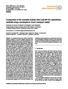
Figure 5.1: Flow chart illustrating ensemble Kalman filter algorithm

27

Chapter 6 An Analytical Comparison of the Two Schemes 6.1

Introduction

Having illustrated the methodologies followed in the two techniques, let us now proceed to make a comparison of the two filters. From the descriptions of the two methods a close similarity is apparent. It is seen that both methods develop a set of realisations for the variable of interest using certain sequential iterative methods, and obtain the best estimate based on these realisations. We would now show that the similarity seen with intuition can be established mathematically. More specifically, we would show that, as the sample size goes to infinity, if at any stage, the particle filter and the ensemble Kalman filter start with the same set of ensemble points, then at the next step, the expected values of the estimates of the ensemble Kalman filter trajectories would be equal to the expectations of the sampling distributions of the particle filter, and the covariances of the individual estimates provided by the ensemble Kalman filter would be equal to the covariances of the mentioned sampling distributions. This effectively means that the ensemble Kalman filter methodologically is an approximated version of the particle filter, without the step involving importance weights. Let us now illustrate a brief outline of the proof. We would first show that the terms involved in the ensemble Kalman filter equations developed at different steps of its derivation would converge in distribution to fixed expressions containing some known matrices. This would follow from the realisation that these terms are approximations of certain covariance quantities related to the state variable θt , the observation variable xt and the noises wt and vt . We would then, under certain restrictions on the ensemble Kalman filter estimates, obtain the expectation and 28

covariance of the estimates given by each estimate. Finally, we would relate these quantities with the expectation and covariance of the particle filter.

6.2

Convergence Results for the Ensemble Kalman Filter Estimates

First let us state our assumptions on the bounds of the ensemble Kalman filter estimates. i Let, at any instant t, and for any trajectory i, t ∈ N, i ∈ {1 · · · Ns }, θˆt,EKF,N s ,α i denote the αth element of the column vector θˆt,EKF,N , α ∈ {1 · · · N }. We assume s i i i ˆ ˆ that for all α, β, and for all i, θt,EKF,Ns ,α , (θt,EKF,Ns ,α )2 and θˆt,EKF,N θî s ,α t,EKF,Ns ,β are all uniformly integrable.

This means that, at any instant t, and for all trajectories i, for every > 0, there exist Kα = Kα (), Lα = Lα () and Cα,β = Cα,β () such that all the following inequalities from 6.1 to 6.3 hold, for all α, β ∈ {1 · · · N }. i sup E[|θˆt,EKF,N |I î s ,α {|θ

t,EKF,Ns ,α |>Kα }

Ns ∈N

i sup E[|(θˆt,EKF,N )2 |I{|(θî s ,α

]Lα }

Ns ∈N

(6.1)

]Cα,β }

Ns ∈N

]