4. Gregory R. Baker and Lan D. Pham different blob method which will converge to a weak solution. The interest here, then, is whether different blob methods ...
1
Under consideration for publication in J. Fluid Mech.
A comparison of blob methods for vortex sheet roll up By G R E G O R Y R. B A K E R1 1
2
AND
L A N D. P H A M2
Ohio State University, Columbus, Ohio, USA
University of California, Irvine, California, USA
(Received 29 September 2004)
The motion of vortex sheets is susceptible to the onset of the Kelvin-Helmholz instability. There is now a large body of evidence that the instability leads to the formation of a curvature singularity in finite time. Vortex blob methods provide a regularization for the motion of vortex sheets. Instead of forming a curvature singularity in finite time, the curves generated by vortex blob methods form spirals. Theory states that these spirals will converge to a classical weak solution of the Euler equations as the blob size vanishes. This theory assumes that the blob method is the result of a convolution of the sheet velocity with an appropriate choice of a smoothing function. We consider four different blob methods, two resulting from appropriate choices of smoothing functions and two not. Numerical results indicate that the curves generated by these methods form different spirals, but all approach the same weak limit as the blob size vanishes. By scaling distances and time appropriately with blob size, the family of spirals generated by different blob sizes collapses almost perfectly to a single spiral. This observation is the next step in developing an asymptotic theory to describe the nature of the weak solution in detail.
2
Gregory R. Baker and Lan D. Pham
1. Introduction Originally, vortex sheets were viewed as models for thin shear layers based on physical intuition. This view has been verified formally by Moore (1978), Baker & Shelley (1990), Dhanak(1994a), and Dhanak (1994b) who show that a vortex sheet is the limit as the thickness of a shear layer vanishes. The assumptions underlying this work are those normally associated with a long wave limit, so, perhaps, it is not too surprising that vortex sheet motion suffers from the spontaneous appearance of singularities as often happens in long wave models. See Cowley, Baker & Tanveer (1999) for both a review and a consistent asymptotic theory that supports the evidence for the formation of a curvature singularity on a vortex sheet in finite time ts . Caflisch & Orellana (1989) establish that singular solutions are closely associated with the ill-posedness of vortex sheet motion. Results from standard applications of numerical techniques to vortex sheet motion have been bedevilled by the onset of irregular motion of the points representing the sheet, driven by the ill-posed nature of vortex sheet motion. Hopes that vortex sheets could be used reliably as models for thin shear flows, such as wakes shed by bodies, were damped, if not dashed. The introduction of vortex blob methods by Chorin & Bernard (1973) and Kuwahara & Takami (1973) opened up new directions for the study of vortex sheet motion. The points representing the vortex sheet are replaced by vortices of prescribed (and fixed) shape. Numerical calculations show regular motion for the centers of the blobs even after ts and, what’s more, the motion shows the formation of a spiral, the expected physical behavior. In particular, Krasny (1986b) uses a special form of the vortex blob method to calculate the roll up of a periodic vortex sheet which results from the classical Kelvin– Helmholtz instability. However, details of the spiral structure depend on the choice of the size of the vortex blob, measured by a parameter δ. Further, there is no direct link
vortex blob methods
3
between the choice of δ and some physical regularization such as the thickness of the shear layer or the presence of viscosity. Comparisons with direct numerical simulations of the viscous motion by Tryggvason, Dahm, & Sbeih (1991) and inviscid layers of small thickness by Baker & Shelley (1990) show good agreement away from the spiral center. Liu & Xin (1995) have placed the use of blob methods for vortex sheet motion on a sound footing by proving that in the limit of δ → 0 the vortex sheet approaches a classical weak solution to the Euler equations. The existence of a weak solution when the vortex sheet strength is of one sign has been established by Delort (1991) and Majda (1993). Of course, the weak solution is unlikely to be unique and will depend on the choice of regularization. The proof of Liu & Xin (1995) uses several assumptions, the one of interest here is that the blob method is the result of a convolution with a suitably defined smoothing function. For example, Krasny (1987) uses an appropriate smoothing function, which has an algebraic decay, to study roll-up of trailing vortices in the wake of an aircraft. Curiously, Krasny (1986b) does not use the periodic version of this blob method but introduces a modified version that has a simple form for periodic motion. The underlying smoothing function is not identified. We derive the smoothing function in this article, and show that it does not satisfy the sufficient conditions of Liu & Xin (1995) for convergence to a weak solution. Nevertheless, numerical results still show apparent convergence as δ → 0. Perhaps the sufficient conditions of Lui & Xin (1995) are not necessary. Beale & Majda (1985) suggest a family of blob methods based on the choice of a Gaussian profile for the smoothing function multiplied by a specific polynomial whose order dictates the degree of accuracy in the approximation. The leading member of this family satisfies the assumptions of the theory of Liu & Xin (1995), and thus provides a
4
Gregory R. Baker and Lan D. Pham
different blob method which will converge to a weak solution. The interest here, then, is whether different blob methods give different weak solutions. We consider four different blob methods: two of them are convolutions with an appropriate smoothing function, and two are regularizations without a clear connection to a convolution with an appropriate smoothing function. Numerical results indicate that the curves form spirals that are different, but approach the same weak limit as δ → 0 for all four cases. For times before ts , the curves calculated with different δ approach the vortex sheet linearly in δ. After ts , the situation is different, For points on the curves away from the spiral region, the convergence is linear, but in the spiral region the convergence is different. Animations of the motion of the spirals suggest they rotate uniformly, and by tracking the angle of the tangent at the spiral center we observe a linear growth in time with the rate of growth dependent on δ. By picking a specific angle θ, we may compare spirals determined with different δ’s geometrically. Of course, the time T it takes the tangent at the spiral center to reach θ depends on δ: the numerical results indicate this dependency is linear for small enough δ. Consequently, by an appropriate scaling in time we may coordinate all spirals with different δ’s to have the same angle for the tangents at their centers. By a further rescaling of distances by δ, the spirals collapse almost perfectly onto one spiral. The results suggest that the spiral may be expressed in a simple form, at least in the limit of vanishing δ, and this form must satisfy a specific version of the vortex sheet equation of motion. However, challenges remain on how to connect the solution to the motion of the vortex sheet outside the spiral.
5
vortex blob methods
2. Mathematical Preliminaries For a comprehensive, detailed treatment of vorticity and the streamfunction we refer the reader to Majda and Bertozzi (2002). Here we simply provide an overview with an emphasis on the origin of blob methods. The velocity u = (u, v) generated by a vorticity distribution ω in two-dimensional flow is given in terms of the streamfunction ψ as (u, v) =
�
∂ψ ∂ψ ,− ∂y ∂x
�
,
(2.1a)
ω(x0 , y 0 ) G(x − x0 , y − y 0 ) dx0 dy 0 .
(2.1b)
where ψ(x, y) = −
Z
∞
−∞
Z
∞ −∞
Here G is the free-space Green’s function for Laplace’s equation ∇2 G(x, y) = δ(x) δ(y)
(2.1c)
and is given as G(x, y) =
� 1 ln x2 + y 2 . 4π
(2.1d )
The velocity may be expressed directly in terms of the vorticity by differentiating (2.1b), leading to integrals containing derivatives of G. These integrals are singular and must be taken in the principal-value sense. These results are valid even when the vorticity is itself singular, for example, when the vorticity corresponds to a vortex sheet, the case of interest in this study. Then, ω = γ(s) δ(n) where n is the normal to the sheet and s the arclength along it from some reference point. Vortex sheets form curvature singularities in finite time where derivatives of the velocity become singular. One way to avoid the formation of singularities is to convolute the velocity with a cutoff function φδ that ensures smooth velocities (uδ , vδ ) and so regularizes
6
Gregory R. Baker and Lan D. Pham
the motion of the sheet. Specifically, uδ (x, y) = = vδ (x, y) = =
∞
Z
∞
Z
−∞ Z ∞
−∞ Z ∞
−∞ Z ∞
−∞ Z ∞
−∞ Z ∞
−∞
−∞ Z ∞
−∞
u(x0 , y 0 ) φδ (x − x0 , y − y 0 ) dx0 dy 0 u(x − x0 , y − y 0 ) φδ (x0 , y 0 ) dx0 dy 0 ,
(2.2a)
v(x0 , y 0 ) φδ (x − x0 , y − y 0 ) dx0 dy 0 v(x − x0 , y − y 0 ) φδ (x0 , y 0 ) dx0 dy 0 .
(2.2b)
From (2.2a) and (2.2b) we see that we may write the velocity in terms of a smoothed streamfunction ψδ (x, y) =
Z
∞ −∞
Z
∞ −∞
ψ(x − x0 , y − y 0 ) φδ (x0 , y 0 ) dx0 dy 0 .
(2.3a)
By substituting (2.1b) into (2.3a), we may express the smoothed streamfunction in terms of the vorticity and a smoothed Greens function Gδ : ψδ (x, y) = Gδ (x, y) =
Z
∞
−∞ Z ∞
−∞
∞
Z
−∞ Z ∞
−∞
ω(x0 , y 0 ) Gδ (x − x0 , y − y 0 ) dx0 dy 0 ,
(2.3b)
G(x − x0 , y − y 0 )φδ (x0 , y 0 ) dx0 dy 0 .
(2.3c)
One of the simplest ways to connect Gδ and φδ is to substitute Gδ into Laplace’s equation 2
∇ Gδ (x, y) =
Z
∞ −∞
Z
∞ −∞
δ(x − x0 ) δ(y − y 0 ) φδ (x0 , y 0 )dx0 dy 0
= φδ (x, y) .
(2.4)
While many choices of φδ will regularize the motion of the curve, the desirable choices are those that ensure the curve approaches a weak solution to Euler’s equations as δ → 0. According to Lui & Xin (1995), the choice φδ (x, y) = φ(x/δ, y/δ)/δ 2 will ensure convergence to a weak limit if φ(x, y) satisfies the following conditions: (i) φ > 0 has continuous second-order derivatives and decays at least as fast as 1/|x| 3 , (ii) Z
∞ −∞
Z
∞
φ(x, y) dx dy = 1 , −∞
(2.5a)
7
vortex blob methods (iii) Z Z
φ(x, y) dx dy ≥
1 . 2
(2.5b)
|x| s2 (δ) > . . . > sm(δ) (δ). With decreasing δ, the spiral has more and more spiral arms. Thus, the number of intersection points m(δ) is an increasing function with decreasing δ. The objective, then, is to study lim sj (δ)
δ→0
17
vortex blob methods 3.7
3.6
KK
KBMK
s1(δ)
3.5
KBM
KBP
3.4
3.3
3.2
0.1
0.15
0.2
0.25
δ
0.3
0.35
0.4
Figure 2. The location of the first outer arm s1 (δ) for all four methods as δ is varied.
and to asses whether the limit is the same for all the kernels. The numerical data consists of the set { (xj , yj ) : 0 ≤ j ≤ N } where xj = x(j4p), yj = y(j4p) and 4p = 2π/N . The functions x(p) − p and y(p) are both odd functions of p. Smooth functions x ˜(p) − p and y˜(p) can be constructed as a sum of sines with the coefficients given by the discrete Fourier transform. Then, the intersection point s i (δ) can be determined by finding the roots of y˜(p). This task is carried out numerically by Newton’s method once the interval in which yj changes sign has been located. The first guess for Newton’s method is the midpoint of the interval. In Figure 2, we plot s1 (δ) at t = 2π for all four kernels. The results suggest strongly that the outer arms all tend to the same limit as δ → 0 but at different rates. The rates clearly depend on the form of the cutoff function. For the two kernels associated with the Gaussian smoothing function the rates are very close. The reason is that the forms are similar as p0 approaches p: the insertion of a factor 2 in the argument of the exponential
18
Gregory R. Baker and Lan D. Pham 3.6
3.58
KBM
3.54
1
s (δ)
3.56
KBMK
3.52
3.5
3.48
0.31
0.315
0.32
0.325
0.33
0.335
δ
0.34
0.345
0.35
0.355
Figure 3. A comparison of s1 (δ) for KBM and KBMK .
of KBMK (2.21) guarantees this since 2
2
cosh(y − y 0 ) − cos(x − x0 ) (x − x0 ) + (y − y 0 ) ≈ 2 δ δ2
2
(3.3a)
when x0 , y 0 are close to x, y. The close agreement of the results is evident in the expanded view of the curves in Figure 3. Similarly, we may compare the expansions of the denominators of the smoothed kernels KBP and KK . From (2.18b) and (2.19), h
cosh
� i (x − x0 )2 + (y − y 0 )2 + δ 2 (y − y 0 )2 + δ 2 − cos(x − x0 ) ≈ 2 2 0 2 (x − x ) + (y − y 0 ) + 2δ 2 cosh(y − y 0 ) − cos(x − x0 ) + δ 2 ≈ 2
�p
The forms match if the δ in KK is replaced by
(3.3b) (3.3c)
√ 2 δ. When δ is rescaled, the curve for
KK falls very closely to that of KBP . Unfortunately, there is no obvious way to connect the δ’s in KBP and KBM . In Figures 4 and 5, we show the results for the second and third arm respectively. They also appear to converge to the same limit as δ → 0, adding further evidence that the weak
19
vortex blob methods
3.45
K
BM
3.4
KBMK
K
BP
3.35
K
2
s (δ)
K
3.3
3.25
3.2
3.15 0.05
0.1
0.15
0.2
δ
0.25
Figure 4. The location of the second outer arm s2 (δ) for all four methods as δ is varied. 3.4
3.35
K
BM
KBP 3.3
,K
BMK
3
s (δ)
KK
3.25
3.2
3.15 0.02
0.04
0.06
0.08
0.1
0.12
δ
0.14
0.16
0.18
0.2
Figure 5. The location of the third outer arm s3 (δ) for all four methods as δ is varied.
limit is the same. The results for the Gaussian kernels are again very close. The results also illustrate that the spirals for the Gaussian kernels are much more tightly wound for the same choice of δ. For example, when δ = 0.2, KK produces one arm of the spiral;
20
Gregory R. Baker and Lan D. Pham
KBP produces two arms; while KBM or KBMK produce at least three arms. Presumably, the short-range influence of the Gaussian smoothing functions, in contrast to the longrange influence of the algebraic decay in the other smoothing functions, produces the more tightly wound spirals. Clearly visible in Figures 4 and 5 is a small oscillatory variation in the curves for the Gaussian kernels. By watching animations of the motion of the spirals the explanation becomes clear. As the spiral center turns and creates a new arm, the remaining arms pulse outwards by a small amount along a radial ray. The larger deviation occurs on the spiral arms nearest the center. Overall, the appearance is that of a travelling wave synchronized on all the arms and rotating uniformly around the spiral center. An important consequence of this wave is that its presence for the choice of kernels K K and KBP , while not easily noticeable, is sufficient to ruin any effort to fit the locations of the arms to a polynomial in δ. Later, we will demonstrate the data matches to a special form. In the meantime, we will confirm that before the singularity time or outside of the spiral region, the sheet does converge linearly in δ. To that end, consider the locations of the Lagrangian markers p = π/4 and p = 3π/4 shown in Figure 1. In Table 2, we give the locations of the markers as δ is decreased at a time t = 0.16 × (2π) = 1.005 before ts . We include the location when δ = 0.0 which must be computed in a special way to avoid the rapid growth of round-off errors as pointed out by Krasny (1986a). He introduced a spectral filter that sets to zero all amplitudes in the Fourier spectrum that fall below a certain level. We also use that filter with N = 512 points and a timestep of 0.000625×(2π). Simultaneously, we can fit the Fourier spectrum to that associated with a branch point singularity in the complex p-plane. Our procedure follows that suggested by Shelley (1992) and Cowley et. al. (1999). By extrapolating the locations of the singularity in δ, we predict the singularity reaches the real axis, and
21
vortex blob methods
p = π/4
p = 3π/4
δ
x
y
x
y
0.10
0.8540464
-0.0693656
2.430926
-0.0709793
0.09
0.8541808
-0.0696088
2.431211
-0.0713376
0.08
0.8543159
-0.0698536
2.431500
-0.0717026
0.07
0.8544515
-0.0701002
2.431796
-0.0720746
0.06
0.8545877
-0.0703484
2.432097
-0.0724537
0.05
0.8547244
-0.0705983
2.432403
-0.0728402
0.04
0.8548617
-0.0784975
2.432716
-0.0732343
0.03
0.8549995
-0.0711029
2.433035
-0.0736364
0.02
0.8551378
-0.0713575
2.433361
-0.0740466
0.01
0.8552766
-0.0716138
2.433694
-0.0744651
0.00
0.8554159
-0.0718716
2.434033
-0.0748924
Table 2. Location of the Lagrangian markers as δ is varied
thus becomes physical, at a time ts = 2.30. This time is slightly earlier than Krasny’s (1986a) time t = 2.36 based on when the tangent of the sheet first becomes vertical. The data in Table 1 for δ 6= 0 falls almost perfectly on straight lines: x(π/4) = 0.8554 − 0.0137 δ
(3.4a)
y(π/4) = −0.0718 + 0.0250 δ
(3.4b)
x(3π/4) = 2.4340 − 0.0307 δ
(3.4c)
y(3π/4) = −0.0748 + 0.0387 δ
(3.4d )
Moreover, their intercepts agree very closely to the values calculated with δ = 0. For the later time t = 2π = 6.283, we have no sheet location for δ = 0, but we may still determine whether the coordinates fall on straight lines in δ. This is true for the Lagrangian marker at p = π/4, but not true for the one at p = 3π/4. In Figure 6 we
22
Gregory R. Baker and Lan D. Pham 1.25
3
1.245
2.95
2.9 1.235 2.85
x((p = 3π/4)
x(p = π/4)
1.24
1.23 2.8
1.225
1.22 0.02
0.03
0.04
0.05
0.06
0.07
0.08
0.09
0.1
2.75 0.11
δ
Figure 6. Variation of the x-coordinates with δ for the two markers p = π/4 (×) and p = 3π/4 (◦). Also shown is the straight line fit to the data for p = π/4.
show the variation of the x-coordinate of the markers p = π/4 and p = 3π/4 with δ. A straight line fit of the data for p = π/4 shows that it falls very closely to a straight line, whereas the data for p = 3π/4 isn’t close to a straight line at all. Our results show that even beyond the singularity formation time regions of the sheet well away from the spiral still converge linearly in δ. On the other hand, the behavior for markers inside the spiral region is different. The way forward is to note that the center of the spiral appears to be in solid body rotation. To confirm this behavior, we study the evolution of the tangent at the the spiral center (p = π). It is easier to display the results as the time Tδ taken to reach the angle θ. The results are shown in Figure 7 for a range of choices in δ. The numerical results are displayed as a series of symbols placed at regular spacings in time. Quite remarkable is the clear indication of a linear relation between Tδ and θ. We have included the best straight line fit Tδ = a(δ) + b(δ)θ
(3.5)
in the range 3 < θ < 40 for each choice of δ and they are displayed as straight lines.
23
vortex blob methods 7 6 5
Tδ
4 3 2 1 0
0
5
10
15
20
25
θ
Figure 7. Time as a function of the sheet angle at the center for δ ranging from 0.01 to 0.10 in steps of ∆δ = 0.1; δ = 0.1 (+), δ = 0.01 (O).
The fits are extremely accurate with a deviation less then 10−4 . Also noticeable is the tendency for the angle to vary very rapidly in time for the smaller values of δ. This rapid variation of the angle means many turns of the spiral form very quickly. The next stage in understanding the limit δ → 0 is to consider the dependency of the slope b(δ) and intercept a(δ) in the straight line fit (3.5). We show the intercept and slope in Figure 8 for the range in δ given in Figure 7. We also show the least squares fit to a cubic polynomial: a = 2.387 + 16.0 δ − 99.06 δ 2 + 379.6 δ 3
(3.6a)
b = −0.00044 + 0.9856 δ + 3.231 δ 2 − 7.386 δ 3
(3.6b)
The accuracy of these form fits is difficult to assess since they have been applied to data that is already the consequence of a straight line fit. The cubic fit to b appears reliable since the cubic term is small over the range in δ. Unfortunately, all terms are important for the cubic fit to a for values of δ ≈ 0.1. However, the visible comparison afforded in Figure 8 is very good.
24
Gregory R. Baker and Lan D. Pham 0.14 3.4
0.12
3.2
0.1 0.08
2.8
0.06
2.6
0.04
2.4
0.02
2.2
0
2
0
0.02
0.04
0.06
0.08
0.1
b(δ)
a(δ)
3
-0.02
δ
Figure 8. The intercept a (×) and slope b (◦) as functions of δ. The solid curves are the least squares fit to a cubic.
One notes that the constant 0.00044 in the cubic fit to b is much smaller in magnitude than the other three constants in the cubic. Further, the impression gained from the curves in Figure 7 is that the slope is becoming horizontal as δ → 0. We assume, therefore, that the constant term in b should really be zero. If this is true, (3.5) should be written as Tδ = 2.387 + 16.0 δ + . . . + (0.9856 δ + 3.231 δ + . . .) θ
(3.7)
or more appropriately when δ is small τ=
t − 2.387 = 16.0 + 0.9856 θ δ
(3.8)
This relation tells us clearly that to study the geometric similarity in the spirals (same θ), we must scale time to keep τ fixed. The origin of τ is t = 2.387 which is very close to estimates for the singularity time ts = 2.356 by Krasny (1986a) and ts = 2.30 by us. Unfortunately, (3.8) proves inadequate to determine the time at which spirals generated with δ in the range (0.01, 0.1) will have the same angle θ at their centers because higher
25
vortex blob methods 0.6 δ = 0.1 0.4
δ = 0.07
y
0.2
0
-0.2
-0.4
-0.6
2.6
2.8
3
3.2
3.4
3.6
x
Figure 9. Vortex sheet locations with δ varying from 0.07 to 0.1 in steps of 0.01. Times are given in the text.
order effects in δ as indicated in (3.6) are important. Instead, we use the form fit (3.5) to determine the time it will take for the spiral to reach an angle θ = 5π at its center. For each choice of δ the time is different: in particular, for δ = 0.1, t = 5.3061; for δ = 0.9, t = 5.0153; for δ = 0.08, t = 4.7249; for δ = 0.07, t = 4.4370; for δ = 0.06, t = 3.8638; for δ = 0.04, t = 3.5738; and for δ = 0.02, t = 2.9956. We display the results in Figure 9 for a limited range in choices for δ simply to maintain clarity in the Figure. Otherwise, the curves overlap and the pattern in the results is obscured. The striking feature of the locations in Figure 9 is that they appear to be evenly spaced. This suggests that the spiral should be scaled according to x ˆ(p) =
x(p) − π δ
and
yˆ(p) =
y(p) δ
(3.9)
We show the consequences of this rescaling in Figure 10. The collapse onto a single spiral is almost perfect. Outside the spiral region, the curves don’t overlap but that is expected. Recall that Lagrangian points outside the spiral region converge linearly in δ when their locations are taken at the same time – see Figure 6. This pattern will be broken when
26
Gregory R. Baker and Lan D. Pham 10
y/δ
5
0
-5
δ = 0.1 δ = 0.02
-10 -10
-5
0 (x-π)/δ
5
10
Figure 10. Rescaled vortex sheet locations for δ = 0.02, 0.04, 0.06, 0.08, 0.1. Times are given in the text.
locations are chosen at different times, as is the case here. On the other hand, the lack of linear convergence for Lagrangian points inside the spiral region can now be understood as the consequence of choosing the locations at the same time instead of the scaled times used here. To pursue this point further, we show the y-coordinate of the vortex sheet as a function of the Lagrangian parameter p in Figure 11 for the cases shown in Figure 9. We have shifted the Lagrangian parameter so that it is centered at the spiral center and we have zoomed onto the region of the spiral. The oscillatory pattern in the y-coordinate illustrates the turns of the spiral. The height of the oscillations reflect the scaling in δ given in (3.9), but what is also apparent is a uniform shift in the location of the peaks of the oscillation. Clearly, the Lagrangian variable should also be scaled, pˆ =
p−π . δ
(3.10)
The results of the scaling, shown in Figure 12, are less impressive than the scaled spirals in Figure 10. There remains a small non-uniform spacing between the curves. There are several possible explanations for the spacing in the curves, the most obvious being that
27
vortex blob methods
0.4 δ = 0.1
y
0.2
0
-0.2 δ = 0.07 -0.4 -1
-0.5
0 p-π
0.5
1
Figure 11. The y-coordinate of the vortex sheet as a function of the Lagrangian variable p for the same cases as in Figure 9.
p − π should be expressed in a power series similar to the one for the time variable (3.7) and that higher order terms in δ are still important. Bearing in mind that that gaps corresponds to a difference of a few percent in the original data, it seems reasonable to assume that the leading order behavior is given by (3.10). In summary, the numerical evidence suggests that after ts , the vortex sheet location behaves as x(p, t) = X(p, t) + δX1 (p, t) . . . ,
(3.11a)
y(p, t) = Y (p, t) + δY1 (p, t) . . . ,
(3.11b)
outside the spiral region, and as �
� p − π t − tc , x(p, t) = π + δF + ... δ δ � � p − π t − tc y(p, t) = δG +... , δ δ
(3.12a) (3.12b)
inside the spiral region. Upon substitution of (3.12) into (2.16),(2.18), we obtain to
28
Gregory R. Baker and Lan D. Pham 8 6 4
y/δ
2
δ = 0.02
0 -2 -4 δ = 0.1 -6 -8 -20
-15
-10
-5
0 (p-π)/δ
5
10
15
20
Figure 12. The scaled y-coordinate of the vortex sheet as a function of the scaled Lagrangian variable p for the same cases as in Figure 10.
leading order Z ∞ 1 ∂F G(ξ, τ ) − G(ξ 0 , τ ) dξ 0 (3.13a) (ξ, τ ) = − � � ∂τ 2π ∞ F (ξ, τ ) − F (ξ 0 , τ ) 2 + G(ξ, τ ) − G(ξ 0 , τ ) 2 + 1 Z ∞ ∂G 1 F (ξ, τ ) − F (ξ 0 , τ ) (ξ, τ ) = dξ 0 (3.13b) � � ∂τ 2π ∞ F (ξ, τ ) − F (ξ 0 , τ ) 2 + G(ξ, τ ) − G(ξ 0 , τ ) 2 + 1
where ξ = (p − π)/δ and τ = (t − ts )/δ.
The first observation about (3.13) that should be made is that a solution exists globally in time because the equations are nothing more than the blob equations with δ = 1. To construct a unique solution we anticipate the need for far-field conditions |ξ| → ∞ and an initial condition at some time τi . Unfortunately, there are no obvious choices for these conditions. We will discuss the issues involved for each condition separately. At first thought, it would seem that the natural initial condition for (3.13) would be at τi = 0, when the singularity would form in the vortex sheet. However, the estimate for ts from the form fit (3.8) is slight later than the estimate based on the trajectory of the branch point singularity in the complex plane. The question arises whether this
29
vortex blob methods 3
2.8 δ = 0.1
Tδ
2.6
2.4
δ = 0.01
2.2
2
0
0.2
0.4
0.6
0.8
1
θ
Figure 13. Time as a function of the sheet angle at the center for δ ranging from 0.01 to 0.10 in steps of ∆δ = 0.1.
occurs because there is another time scale close to the singularity formation during which the curve adjusts prior to settling into a late time pattern. A close examination of the tangent angles at the center as they evolve in time is shown in Figure 13. The results are the same as in Figure 7 except curves are drawn in place of discrete values and the straight line fits have been removed. The question that must be resolved is whether the curves indicate a dependency of the form θ = f (τ ). If this form is correct, then (3.13) will describe the transition of the curves from before the singularity time τ