A Comparison of Methods for Optimising Resource

A Comparison of Methods for Optimising Resource Plans Simon M. Miller Centre for Computational Intelligence De Montfort University Leicester, LE1 9BH, UK [email protected]

Mario Gongora Centre for Computational Intelligence De Montfort University Leicester, LE1 9BH, UK [email protected]

Abstract Planning resources for a supply chain is a major factor determining its success or failure. In this paper we take an existing Interval Type-2 Fuzzy Logic resource planning model, and compare the performance of a Genetic Algorithm, Simulated Annealing, the Great Deluge Algorithm and hybrid optimisation methods combining the GA with each of the other methods. Each method is used to search for good resource plans that meet a service level requirement while minimising cost. A discussion of the results of the experiment is given along with considerations for future research.

1 Introduction Optimising inventory levels within a supply chain is an area of ongoing interest for supply chain managers. Planning the allocation of resources within a supply chain (SC) has been critical to the success of manufacturers, warehouses and retailers for many years. Mastering the flow of materials from their creation to the point of sale offers considerable advantages for those within a well managed SC. Poorly managed resources result in two main problems: stock outs and surplus stock. The consequence of stock outs is lost sales, and potentially lost customers. Surplus stock results in added holding cost and the possibility of stock losing value as it becomes obsolete. Holding some surplus stock is advantageous however; safety stock can be used in the event of an unexpected increase in demand or to cover lost productivity. Various degrees of uncertainty are present in the different data sources used in Supply Chain Management (SCM). This uncertainty is further amplified in demand forecasts by applying methods of analysis with (again) varying degrees of inherent uncertainty. Furthermore, other data that is often used in resource planning such as transportation and other costs, customer satisfaction information, etc. is also uncertain.

Viara Popova Centre for Manufacturing De Montfort University Leicester, LE1 9BH, UK [email protected]

Therefore, Fuzzy Logic (FL) and especially Type2 Fuzzy Logic (T2FL) are particularly appropriate for this problem. While Type-1 FL (T1FL) has successfully been used many times for modelling SC operation (see Section 2), T2FL has been shown to offer a better representation of uncertainty on a number of problems (e.g., Hagras (2004) and Karnik and Mendel (1999)). In Miller et al. (2009) the authors applied Interval Type-2 Fuzzy Logic (IT2FL) to a 2tier distribution resource model and it was shown to work well. In this paper we compare the performance of a Genetic Algorithm (GA), Simulated Annealing (SA) and the Great Deluge Algorithm (GDA) on a multiple tier IT2FL resource optimisation problem. In addition to this, tests using hybrid methods that combine the use of a GA with SA, and a GA with GDA will be reported. We believe that the best aspects of each algorithm can be exploited by combining them in one process. To date, neither the GDA nor the hybrid methods mentioned have been applied to an IT2FL model of this kind. In Section 2 the optimisation techniques and their applications in related work are discussed. Following this is an overview of T2FL and the model being used for the study, with a description of the test scenario. The experiments will compare the performance of the optimisation methods on the test scenario problem.

2 Fuzzy resource model optimisation There are a number of research projects that have explored the use of optimisation techniques with T1FL models. In this section we will look at GAs, SA and the GDA with examples of their use. Genetic Algorithms (GAs) are a popular method of optimising fuzzy resource models. A GA (Holland, 1975) is a heuristic search technique inspired by evolutionary biology. Selection, crossover and mutation are applied to a population of individuals representing solutions in order to find a near-optimal solution. Like the other methods considered here,

the GA is able to find good solutions to a problem while evaluating only a small fraction of the solution space. For an optimisation method to be practical, this is critical, as resource planning tends to involve an extremely large solution space. In Aliev et al. (2007) a type-1 fuzzy system is used with a GA to model a SC. The GA searches for a configuration that maximises profit, while meeting a target fillrate specified by the user; fuzzy sets are used to describe costs, returns, production capacities, storage capacities and forecasts. The proposed fuzzy method, and a crisp method are compared. The crisp system is unable to produce a feasible configuration if the actual demand is lower than the forecast. In contrast, the fuzzy model presented is robust and able to cope with fluctuation in demand and production capacity with little impact on profitability. A similar approach is presented by Wang and Shu (2005). T1FL is used to represent customer demand, processing time and delivery reliability; a GA finds order-up-to levels. The system attempts to find the configuration that incurs the minimum cost. An optimism-pessimism index is set by the user and passed to the system. When optimistic, the model assumes the best case scenario for material response time. A pessimistic attitude presumes the worst. The results show that more pessimistic strategies increase the fill rate, reducing the sales lost through stock outs, and incur higher inventory cost as more stock is kept. More optimistic strategies result in a drop in fill rate and an increase in sales loss, though inventory cost is also reduced. Fayad and Petrovic (2005) carried out work using a T1FL job scheduling model with a GA to find near-optimal solutions. In this case a real world example (a printing company) is used to demonstrate the model. Fuzzy sets are used to describe due dates, processing times and the level of satisfaction. The experiments described show that the GA is able to find good solutions. Earlier work by Sakawa and Mori (1999) also describes a method of scheduling jobs that have a type-1 fuzzy due date and processing time. A GA is used to find schedules. The GA takes into account the similarity of the solutions in a given population. When the initial individuals are created they have a similarity of 0.8 or less to ensure diversity. It is shown that ensuring diversity in this way leads to the GA finding an optimal solution on more occasions than a GA without a similarity measure. In testing, the GA is shown to work well, finding solutions with a large correlation between the processing time and the due date. For comparison, a Simulated Annealing process is used. Like GAs, Simulated Annealing (SA) (Kirk-

patrick et al., 1983) is inspired by a real-world phenomenon, in this case the heating and cooling (annealing) of metals to reduce defects. An initial solution is created, then a neighbouring solution is selected and compared with it. The probability of the algorithm accepting the neighbour as the current solution is based upon a temperature value and the difference in quality between the two solutions. The higher the temperature value, the more likely it is that the algorithm will accept an inferior solution. The process is then repeated using the selected solution as a starting point. Over the course of a run the temperature is gradually decreased. SA has been successfully applied to a number of optimisation problems. For example in Tang (2004) a series of experiments are described that show SA is an appropriate choice for optimising a production/inventory system. Melouk et al. (2004) and Bouleimen and Lecocq (2003) use SA to solve production scheduling problems. In the tests done in Sakawa and Mori (1999) the GA is shown to consistently outperform the SA method used. Not only are the solutions better, but the results are more stable. The variance in the best solutions found with SA from test to test is much larger than that of the GA. The computation time for the GA is also shown to be faster. The Great Deluge Algorithm (GDA) (Dueck, 1993) is proposed as an alternative to SA, and works in a similar manner. The GDA is inspired by the idea of a person or animal attempting to escape a flood. As with SA an initial solution is created, then a neighbouring solution is selected. To be accepted as the current solution, the neighbouring solution need only be above a water level value. To begin with, the water level is very low, meaning inferior solutions are likely to be accepted. As time goes on however, the water level increases, meaning solutions have to be better and better to be accepted. The result is that the algorithm wanders around the solution landscape looking for higher and higher ground until it is stranded on a high point. After a number of iterations has passed without improvement, the algorithm is terminated. While the GDA has been used with success on other types of problem (for example, exam timetabling in Burke et al. (2004)), it has yet to be used with a fuzzy resource planning model. By combining methods it is believed that the best aspects of each algorithm can be exploited. There exists a large body of work demonstrating the benefits of combining a GA and SA in one search (e.g., Adler (1993) and Li et al. (2002)), some use a hybrid algorithm to find solutions for type-1 fuzzy models (e.g., Wong and Wong (1996) and Wong and Wong (1997)). Currently there are no examples in the literature of using this method to optimise a type-2

model configuration. A GA is able to find consistently good solutions, but requires a large population and therefore is computationally expensive. Conversely, SA avoids the problem of maintaining a large population, but to a great extent its success relies on the location of the initial random individual. By combining these methods we can allow the GA to find a good region of the search space, and then let SA take over to reach the peak in this region more efficiently. The GDA can be used in the same way. Like SA, the GDA does not require a large population, but is affected by the location of the initial random solution. In this paper, we will apply a GA, SA and the GDA to an IT2FL resource planning model individually, and then proceed to test GA-SA and GA-GDA hybrids on the same problem. As stated before, there are no examples of using these hybrid algorithms to optimise an IT2FL resource model; this paper will report the first results in an ongoing project. 2.1 Type-2 Fuzzy Logic (T2FL) In the examples given we have seen how T1FL has been used to tackle the resource planning problem. However type-1 fuzzy sets represent the fuzziness of the particular problem using a ‘non-fuzzy’ (or crisp) representation - a number in [0, 1]. As Klir and Folger (1988) point out: “..it may seem problematical, if not paradoxical, that a representation of fuzziness is made using membership grades that are themselves precise real numbers.” This paradox leads us to consider the role of type-2 fuzzy sets as an alternative to the type-1 paradigm. Type-2 fuzzy sets (Mendel and John, 2002) represent membership grades not as numbers in [0, 1], but as type-1 fuzzy sets. Type-2 fuzzy sets have been widely used in a number of applications (see John and Coupland (2007) and Mendel (2007) for examples), and on a number of problems T2FL has been shown to outperform T1FL (e.g., Hagras (2004) and Karnik and Mendel (1999)). In previous work (Miller et al., 2009) the authors have shown that Interval Type-2 Fuzzy Logic (IT2FL) (Mendel et al., 2006) is an appropriate method of modelling a 2-tier distribution network. IT2FL has been used because it is computationally cheaper than general T2FL as it restricts the additional dimension, referred to as the secondary membership function, to only take the values 0 or 1. We believe that the extra degree of freedom will allow a better representation of the uncertain and vague nature of data used in SCM.

2.2 Model The IT2FL model used for the experiments represents the interaction of nodes within a multiple echelon supply chain over multiple periods of time. In each echelon there are one or more nodes that supply the subsequent echelon with one or more products, and receive stock from the preceding echelon. The first echelon receives goods from an external supplier which is assumed to have infinite capacity, the final echelon supplies the end customer. Customer demand is provided by a fuzzy forecast which is given to the model at run-time. This forecast represents the demand placed upon the final echelon in the SC. Echelons above this can see their own demand by looking at the suggested inventory levels at the succeeding echelon, as they will be required to supply these items. Solutions (resource plans) take the form of a matrix representing the inventory level of each product, at each node, in each tier, in each period. The following values are represented by IT2FL fuzzy numbers: forecast demand, inventory level, transportation distances, transportation cost, stock out level, stock out cost, carry over, carry cost and total cost. Fuzzy numbers are produced by taking crisp numbers, and creating triangular fuzzy sets where the crisp number has a µ value of 1, and the set extends to values 2.5 either side of the given x value. To make the sets IT2FL, this set is blurred to cover values 0.5 either side of the type-1 set.

3 Test scenario To compare the performance of each optimisation method, a scenario has been created. In the scenario the SC consists of 4 echelons (including the end customers), with 2 nodes in each. There are 2 products, and the model is to be run for 6 periods. The resource plan found will need to achieve a customer service level of at least 95%. Each customer requires about 200 items of each product in each period, and each node can handle a maximum of 500 items of each product per period. Table 1 gives the operating costs of the supply chain. To calculate transport costs, the model needs to know the distance between nodes. Table 2 shows the distances between nodes in successive echelons. A tilde (e.g., ˜100) denotes a fuzzy number. To find a good cost for comparison a resource plan was created that matched demand in each period, using nodes that are closest to one another. When put into the model, a cost of £529,287.31 was produced. It should be noted that this plan will satisfy 100% of customer orders, the test scenario will allow solutions that satisfy 95% of orders and as

Batch cost Production cost Transport cost Purchase value Holding cost

Product 1 2 £100 £30 £40 ˜£2 ˜£3 £50 £70 £5 £7

Table 1: Supply chain costs

Src. node Echelon 1 Node 1 Node 2 Echelon 2 Node 1 Node 2 Echelon 3 Node 1 Node 2

Dest. node 1 2 ˜100 ˜200

˜200 ˜100

˜200 ˜100

˜100 ˜200

˜100 ˜200

˜200 ˜100

Table 2: Supply chain distances such may be cheaper. 3.1 Optimisation setup Experiments with previous versions of the model ((Miller et al., 2008) and (Miller et al., 2009)) have produced a GA setup that has been shown to work well for fuzzy resource planning problems. We use this setup for our experiments here. The configurations of the other methods presented were decided upon by carrying out some initial experimentation. For all methods, fitness is judged by calculating the total cost of candidate solutions. A penalty is added to solutions that do not meet the customer service requirement in proportion to the cost, and the distance between the actual and target service levels. The optimisation methods have been configured as follows: Genetic Algorithm The population consists of 250 individuals, and the algorithm is run for 500 generations. New generations consist of: 1% individuals produced with elitism, 20% copied individuals, 20% individuals created with single point crossover and 59% of individuals created using mutation. Simulated Annealing The temperature needs to be set sufficiently high to encourage initial exploration, without introducing unneccessary computation. For example, early experimentation with SA on the previous version of the model seen in Miller et al. (2009) showed that a temperature of 800 allowed for sufficient exploration of the solution space. When

the same setup was used with the current model, the results were poor. This is because the values that the current scenario and model produce are significantly higher, and the solution space is much larger. The low temperature was not encouraging exploration, and so was raised. The initial temperature is set to 10,000, the temperature is reduced by 10 after 300 iterations or if 150 iterations pass without improvement. The algorithm terminates when the temperature reaches zero. Great Deluge Algorithm As our problem is to minimise a value, for simplicity we have reversed the GDA so that the water level starts high, and then decreases. The water level needs to be set at a level appropriate to the problem. In early tests we found the the water level should be set slightly above the likely value of the initial solution, in this case around 1,900,000. The initial water level is set to 2,000,000, the level is reduced by 25 each time a new solution is accepted and the algorithm terminates after 1,500 iterations with no improvement. Genetic Algorithm-Simulated Annealing The GA is configured as before, but only runs for 50 generations. The SA algorithm has an initial temperature of 4,500, which is reduced after 300 iterations with improvement or 150 iterations without improvement. A lower temperature is used as the GA has already completed an initial search to find a good region of the solution space, and we do not want to encourage too much exploration. Genetic Algorithm-Great Deluge Algorithm The GA has a population of 250 and runs for 150 generations. The water level is reduced to take into account that the initial individual is not random and therefore will be of higher quality. The initial water level is set to 725,000. The water level is reduced by 25 in each iteration and the algorithm terminates after 1,500 generations without improvement.

4 Results Each method was tested 10 times with differing random seeds. Table 3 shows the mean cost of the best solutions found in each test, the standard deviation and the mean time taken in seconds. All of the resource plans found had a service level of 95.83%. In the individual tests (GA, SA and GDA), SA performed the best. As well as finding the cheapest solutions, it was also more consistent than both the GA and the GDA. The GDA was the poorest in these tests, as it was not able to find solutions that matched the other methods, and also the result varied a great deal depending upon the random seed used. Of the hybrid methods (GA-SA and GA-GDA)

Method

Mean cost £509364.63 £464013.36 £512554.44 £470136.62 £518409.22

GA SA GDA GA-SA GA-GDA

Std. dev. 6977.86 6113.84 12579.89 4678.43 8060.98

Mean time 2029.5s 2179.6s 1795.8s 1060.1s 910.0s

Table 3: Results of optimisation experiments - Mean best solutions found

1,600,000

Cost of best solution found (£s)

GA 1,400,000 1,200,000 1,000,000 800,000 600,000 400,000

0

50

100

150

200 250 300 350 Number of Generations

400

450

500

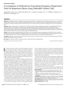
(a) GA 2,200,000 GDA SA


2,000,000 1,800,000 1,600,000 1,400,000 1,200,000 1,000,000 800,000 600,000 400,000

0

25,000

50,000

75,000 100,000 125,000 Number of Iterations

150,000

175,000

(b) SA & GDA 900,000 SA

come, finding solutions within 1.1% of those found with GDA alone in 49.44% less time. Again, consistency was improved, but it still did not match the consistency of the other optimisation methods. We can see how combining the algorithms can improve their performance by looking at Figures 1(a), 1(b) and 1(c). The first two graphs show how cost changes over the best run of the GA, SA and GDA. With the GA (Figure 1(a)), there is a sharp improvement initially, then after approximately 150 generations the improvements slow down. With SA, the cost also decreases sharply in the beginning like the GA, but solutions continue to fluctuate for a greater proportion of the run. With GDA the improvements are more gradual. Figure 1(c) shows the SA component of the best GA-SA run. This shows the improvements made by SA after the algorithm has been passed a solution by the GA. The GA has 1 of the generations in the run for 50 generations ( 10 GA test), and it can be seen that SA settles after around 25,000 iterations, less than 14 of the iterations taken in the SA test. 1 of the The combination of running the GA for 10 generations used in the GA test, then using SA to reach a near-optimal solution in less than a quarter of the time taken in the SA test, results in an algorithm that is able to find solutions close to the quality of SA in less than half the time of each method individually. The speed of stability achieved by SA in GA-SA makes clear that the starting point provided by the GA is better than starting SA from a random location. The GA finds a better region of the search space, once in this region SA is able to find better solutions and reach a minimum quicker than using the GA alone.

5 Conclusion


850,000 800,000 750,000 700,000 650,000 600,000 550,000 500,000 450,000

0

12,500

25,000 37,500 50,000 Number of Iterations

62,500

75,000

(c) GA-SA - SA component of the run

Figure 1: Improving best solutions GA-SA achieved the best results as we might expect. The tests showed that GA-SA was able to find solutions comparable (on average 1.3% higher) to those found in the SA tests in 52.4% less time. The GASA hybrid algorithm was also the most consistent of those tested. The GA-GDA produced a similar out-

In this paper we have presented a comparison of three individual optimisation methods, and two hybrid methods. Experimentation has shown that individually, SA provides us with the best performance. However, we have also seen that by combining a GA with SA we can obtain the benefits of both methods to achieve the lower costs SA finds, in much less time. Another outcome of the work is that it has illustrated the sensitivity of the algorithms to their settings. Although a good temperature and water level were discovered for this problem, taking these settings and applying the algorithm to another problem would yield unpredictable results. Further work in this area could include a more thorough investigation of each method’s sensitivities to parameters, and looking at methods for calculating temperature (or water level) based on the space of solutions to be

searched. For the GDA’s water level this could be as simple as taking the initial solution and adding a value to it, for SA it might be that we can calculate a proportion of the initial value that should be used.

Acknowledgment The research reported here has been funded by the Technology Strategy Board (Grant No. H0254E).

References D. Adler. Genetic algorithms and simulated annealing: A marriage proposal. In Proceedings of the IEEE International Conference on Neural Networks, volume 2, pages 1104–1109, 1993. R.A. Aliev, B. Fazlollahi, B.G. Guirimov, and R. R. Aliev. Fuzzy-genetic approach to aggregate production-distribution planning in supply chain management. Information Sciences, 177:4241– 4255, 2007. K. Bouleimen and H. Lecocq. A new efficient simulated annealing algorithm for the resourceconstrained project scheduling problem and its multiple mode version. European Journal of Operational Research, 149(2):268–281, 2003. E.K. Burke, Y. Bykov, J.P. Newall, and S. Petrovic. A time-predefined local search approach to exam timetabling problems. IIE Transactions on Operations Engineering, 36(67):1–19, 2004. G. Dueck. New optimization heuristics: The great deluge algorithm and record-to-record travel. Journal of Computational Physics, 104:86–92, 1993. C. Fayad and S. Petrovic. A fuzzy genetic algorithm for real-world job shop scheduling. In Proceedings of the 18th international conference on Innovations in Applied Artificial Intelligence. Bari, Italy., pages 524–533, 2005. H.A. Hagras. A hierarchical type-2 fuzzy logic control architecture for autonomous mobile robots. IEEE Transactions on Fuzzy Systems, 12(4):524– 539, August 2004. J.H. Holland. Adaptation in natural and artificial systems: an introductory analysis with applications to biology, control, and artificial intelligence. Ann Arbor: University of Michigan, 1975. R.I. John and S. Coupland. Type-2 fuzzy logic a historical view. IEEE Computational Intelligence Magazine, 2(1):57–62, February 2007. N.N. Karnik and J.M. Mendel. Applications of type-2 fuzzy logic systems to forecasting of timeseries. Information Sciences, 120:89–111, 1999. S. Kirkpatrick, C.D. Gelatt Jr., and M.P. Vecchi. Optimization by simulated annealing. Science, 220

(4598):671–680, May 1983. G.J. Klir and T.A. Folger. Fuzzy Sets, Uncertainty and Information. Prentice Hall, 1988. W.D. Li, S.K. Ong, and A.Y.C. Nee. Hybrid genetic algorithm and simulated annealing approach for the optimization of process plans for prismatic parts. International journal of production research, 40(8):1899–1922, 2002. S. Melouk, P. Damodaran, and P.Y. Chang. Minimizing makespan for single machine batch processing with non-identical job sizes using simulated annealing. International Journal of Production Economics, 87(2):141–147, 2004. J. M. Mendel. Advances in type-2 fuzzy sets and systems. Information Sciences, 177(1):84–110, January 2007. J.M. Mendel and R.I.B. John. Type-2 fuzzy sets made simple. IEEE Transactions on Fuzzy Systems, 10(2):117–127, April 2002. J.M. Mendel, R.I. John, and F. Liu. Interval type-2 fuzzy logic systems made simple. IEEE Transactions on Fuzzy Systems, 14(6):808–821, December 2006. S.M. Miller, V. Popova, R. John, and M. Gongora. Improving resource planning with soft computing techniques. In Proceedings of UKCI 2008, De Montfort University, Leicester, UK., September 2008. URL available at: http://www.cci.dmu.ac.uk/preprintPDF/ SimonUKCI(2).pdf. S.M. Miller, V. Popova, R. John, and M. Gongora. An interval type-2 fuzzy distribution network. In Proceedings of 2009 IFSA World Congress/EUSFLAT Conference, Lisbon, Portugal, July 2009. M. Sakawa and T. Mori. An efficient genetic algorithm for job-shop scheduling problems with fuzzy processing time and fuzzy duedate. Computers & Industrial Engineering, 36:325–341, 1999. O. Tang. Simulated annealing in lot sizing problems. International Journal of Production Economics, 88(2):173–181, 2004. J. Wang and Y-F. Shu. Fuzzy decision modelling for supply chain management. Fuzzy Sets and Systems, 150(1):107–127, 2005. K.P. Wong and Y.W. Wong. Combined genetic algorithm/simulated annealing/fuzzy set approachto short-term generation scheduling with take-or-pay fuel contract. IEEE Transactions on Power Systems, 11(1):128–136, 1996. K.P. Wong and Y.W. Wong. Hybrid genetic/simulated annealing approach to shorttermmultiple-fuel-constrained generation scheduling. IEEE Transactions on Power Systems, 12(2):776–784, 1997.