Paper presented at the 22nd Asian Conference on Remote Sensing, 5 - 9 November 2001, Singapore. Copyright (c) 2001 Centre for Remote Imaging, Sensing and Processing (CRISP), National University of Singapore; Singapore Institute of Surveyors and Valuers (SISV); Asian Association on Remote Sensing (AARS) ____________________________________________________________________________________________
A COMPARISON OF EMPIRICAL ALGORITHMS FOR CHLOROPHYLL CONCENTRATION IN SINGAPORE REGIONAL WATERS Md. Monirul Islam Research Fellow Tropical Marine Science Institute National University of Singapore 14 Kent Ridge Road, Singapore 119223 Tel: +65 874 4649, Fax: +65 872 4067 E-mail:
[email protected] Chan Weng Tat Associate Professor Department of Civil Engineering National University of Singapore 10 Kent Ridge Road, Singapore 119260 Tel: +65 874 2576, Fax: +65 779 1635 E-mail:
[email protected]
KEYWORDS: SeaWiFS data, SeaDAS, band ratio, chlorophyll ABSTRACT: The subject of this study is ocean color monitoring of the regional waters around Singapore. Remote sensing reflectance measurements were used to evaluate the performance of several published ocean color chlorophyll algorithms for use with SeaWiFS (Sea-viewing Wide Field-of-view Sensor) data. The radiancechlorophyll data were assembled from various SeaWiFS images spanning over a one - year period. Using the default chlorophyll algorithm (OC4-v4) used in SeaDAS (SeaWiFS Data Analysis System) as the basis of comparison, the study examined the characteristics of fifteen empirical chlorophyll/pigments algorithms. The results obtained in the study indicated that the chlorophyll-a concentration predictions could be categorized roughly into three regions: the first region ranges from 0.1 to 1 mg/m3 , the second from 1 to 5mg/m3 and the last region for chlorophyll-a concentrations greater than 5.0 mg/m3 . The algorithms Aiken-C, Aiken-P, CalCOFI-1, OC1a, OC1b, OC2-V2 and OC2-v4 show nominal divergence for the three regions; CalCOFI-2, OC1c, OC1d, OC2 and OC2c show nearly the same profile for the first region, nominal divergence in the second region but show the greatest amount of divergence compared with SeaDAS default chlorophyll concentration calculated by OC4-v4 in the third region. The Morel 4 algorithm shows much higher divergence of chlorophyll concentration for all three regions, whilst CAL-P6 shows nominal deviation for the second and third regions. In the third region, the values estimated by all algorithms show much more deviation from the SeaDAS default values, especially at higher chlorophyll-a concentrations. Aiken-P shows the least root mean square value (0.290691) of the divergence from the SeaDAS default algorithm, followed by OC2-v2 (0.59598), Aiken-C (0.855854), OC2-v4 (0.979607) and so on. 1. INTRODUCTION Satellite ocean color research began in the late 1970s with the coastal zone color scanner (CZCS) aboard the Nimbus 7 satellite which acquired data from October 1978 to June 1986 (Evans and Gordan, 1994; Acker, 1994). More than a decade after the end of the pioneer coastal zone scanner mission, a new generation of ocean color sensor SeaWiFS has emerged. Since the launch of the SeaWiFS aboard the SeaStar satellite in August 1997 (Chuanmin et al., 2000), global ocean color data has been available to scientists on a regular basis. SeaWiFS is superior to the original Coaster Zone Color Scanner (Hovis et al., 1980; Chuanmin et al., 2000). It has much more higher radiometric sensitivity and additional spectral bands to aid in atmospheric correction and bio-optical applications. This new sensor has more wave bands and higher precision and is designed to avoid some of the limitations of the CZCS (Hooker et al., 1993, Kahru and Mitchell, 1999). Satellite ocean color data provides the only practical means for monitoring the spatial and seasonal variation of near surface phytoplankton, information essential for the study of oceanic primary production, global carbon and other biological cycles, as well as for fisheries research. The influence of phytoplankton on the ocean color of seawater has been studied for several decades. It is well understood that chlorophyll-a, the primary photosynthetic pigment in phytoplankton, absorbs relatively more blue and red light then green, and the spectrum of backscattered sunlight or color of ocean water progressively shifts from deep blue to green as the concentration of phytoplankton increases (O,Reilly et al, 1998). In this study, SeaWiFS data was used to view the ocean color in the regional seas around Singapore. Data sets were downloaded from NASA Goddard Space Flight Centre and analysed using the SeaDAS software developed by NASA.
We briefly review the fifteen algorithms, derived from two band ratios: band 3 (490nm) and band 5 (555nm) for chlorophyll concentration, and we also present their suitability for operational use compared with the default SeaDAS algorithm. Most of the algorithms were developed by using SeaBAM (SeaWiFS Bio-optical Algorithm Mini-Workshop) and CalCOFI (the California Cooperative Oceanic Fisheries Investigations) data sets (O’Reilly et al., 1998; Kahru and Mitchell, 1999). 2. DATA PREPARATION AND SELECTED ALGORITHMS 2.1 SeaDAS software for data preparation and deriving chlorophyll concentration SeaWiFS LIA data was collected from NASA. The data files contain the reflectance data obtained for each of the eight SeaWiFS electromagnetic bands. Metadata like time of scanning, position of the scanned areas, characteristic of sensor during the scanning session etc. are also included in these files. The large size of each full scene file (70100 MB) puts a strain on processing time and physical storage space. To alleviate this, only the required portion corresponding to the area of interest was extracted. This area covered the whole of Singapore, part of Malaysia, Sumatra, Straits of Malacca and the South China Sea and is generally between latitude 6~-2o and longitude 98~109o . SeaDAS software was used to prepare the SeaWiFS data. The L1A SeaWiFS data only gives the reflectance measurements for each of the eight bands. An atmospheric correction procedure is first carried out to reduce the errors of both the water-leaving radiance and the chlorophyll concentration estimates (Chuanmin et al., 2000). Bio optical algorithms are then employed to create a level 2 end products. There are 176 level 2 products available for selection in the SeaDAS software. Any combination of these 176 products may be selected for output and written to physical files. The output products include 8 bands across 17 radiance categories like normalized water leaving radiance (Lnw), water leaving radiance (Lw), Rayleigh radiance, aerosol radiance, ozone transmittance (sun to ground, and ground to sensor), total oxygen transmittance, etc. There are also 40 additional miscellaneous products like chlorophyll concentration (using various algorithms like OC2, OC4-v4, Neural Net Pigment etc), pigment concentration (derived from chlorophyll concentration products), sensor and solar zenith, and azimuth angle. One of the products, L2_flags, allows certain flags to be used as masks. Processing is bypassed for masked pixels and the output value is set to zero. This product can be applied for land, sun glint, total radiance greater than the knee value, large sensor zenith angle, clouds, etc. Using the SeaDAS OC4-v4 algorithm, chlorophyll concentrations were estimated for several images for the selected areas. Similarly, Lwn files for band 3 and band 5 were prepared for the corresponding images. 2.2 Selected Algorithms Many empirical models, with varying degrees of complexity, have been proposed within the last two decades to relate the backscattering properties observed to the concentration of dissolved substances in the water column. These models may use information in single or multiple bands, and employ different functional forms like the power function, multiple regression hyperbolic, second-order and third-order polynomials, or most commonly the log-transformation. NASA convened a small working group at the SeaWiFS Bio -optical Algorithm MiniWorkshop (SeaBAM) with the goal of identifying suitable algorithms for the estimation of chlorophyll a (C) and chlorophyll a plus phaeo-pigments (C+P) from SeaWiFS data on an operational basis (Fireston and Hooker, 1998; O’Reilly et al., 1998). Altogether, fifteen empirical algorithms (Table 1) identified during the workshop, as well as others suggested by S. Maritorena, and Kahru and Mitchell (Kahru and Mitchell, 1999) were evaluated in this study on the area of interest. Some of the algorithms require remote sensing reflectance, Rrs, and others require normalized water leaving radiance, Lwn. The formulae for Aiken-C, Aiken-P, CalCOFI-1 (two band power), CalCOFI-2 (two band cubic), Morel 2, Morel 4, OC1a, OC1b, OC1c, OC1d, OC2, OC2-v2, OC2c, OC2-v4 and CAL-P6 are shown in Table 1. The Aiken hyperbolic models estimates chlorophyll (C) and the combination of chlorophyll and pigments (C+P) by the comb ination of a hyperbolic function up to 2 µmL-1 with a power function at higher concentrations (Aiken et al., 1995) using a 2-band ratio Lwn490/Lwn555. The CalCOFI algorithms were derived from CalCOFI data (Mitchell and Kahru, 1998) and estimate chlorophyll using a power equation of a 2-band ratio Rrs490/Rrs555. The Morel-2 algorithm uses the band ratio Rrs490/Rrs555 and Morel-4 is a cubic polynomial with Rrs490/Rrs555, which was derived from in situ measurements and an updated version of the Morel (Morel 1988) semi analytic model (O’ Reilly, 1998). The empirical chlorophyll algorithms OC1a to OC1d and OC2 were tuned to the SeaBAM data.
Table 1. Empirical Algorithms Algorithm
Type
Equations
Band ratio (R) & Coefficients (a)
Aiken-C
Hyperbolic +power
C 21 = exp(a0 + a1* ln( R ))
If [C + P ] < 2.0µgL−1 then [C + P ] = C 24
R = Lwn 490/ Lwn555 a = [ 0.464, −1.989, − 5.29, 0.719, − 4.23] R = Lwn490/ Lwn555 a = [ 0.696, − 2.085, − 5.29, 0.592, − 3.48]
Aiken-P
Hyperbolic +power
C 23 = ( R + a2) /(a3 + a 4 * R ) C = C 21 ; if C < 2.0µgL−1 then C = C 23 C22 = exp(a0 + a1* ln(R )) C24 = (R + a 2) /(a3 + a4 * R ),[C + P ] = C 21
CalCOFI two band
Power
C = 10 ( a 0 + a1* R )
R = log(Rrs490/ Rrs555)
CalCOFI two band
Cubic
C = 10
a = [0.444, − 2.431] R = log(Rrs490/ Rrs555)
Morel 2
Power
C = exp( a 0 + a1 * R )
Morel 4
Cubic
C = 10 ( a 0 + a1* R + a 2 *R
OC1a
Power
OC1b
Geometric
OC1c
Quadratic polynomial
OC1d
( a 0 +a1*R + a 2* R 2 +a 3* R3 )
a = [ 0.450, − 2.86, 0.996, − 0.3674]
R = ln( Rrs 490 / Rrs 555 ) a = [1 .077835 , − 2.542605 ] R = log( Rrs 490 / Rrs 555 ) a = [1.03117 , − 2.40134
+ a 3* R 3 )
2
0 .3219897 , − 0.291066 ] C = 10
( a 0 + a1* R )
R = log(Rrs490/ Rrs555)
C = 10
( a 0 +a 1* R )
a = [ 0.3734, − 2.4529] R = log(Rrs490/ Rrs555)
C = 10
( a 0 +a 1* R + a 2 *R 2 )
Cubic polynomial
C = 10
( a 0+ a 1* R + a 2 *R 2 + a 3* R 3 )
OC2
Modified cubic polynomial
C = 10 (a 0 +a 1* R + a 2* R
2
+a 3*R 3 )
+ a4
OC2-v2
Modified cubic polynomial
C = 10 (a 0 +a 1* R + a 2* R
2
+a 3*R 3 )
+ a4
OC2c
MCP
C = 10 (a 0 +a 1* R + a 2* R
2
+a 3*R 3 )
+ a4
OC2-v4
MCP
C = 10
CAL-P6
Sixth order polynomial
C = 10 ( a 0 + a1*R + a 2 * R
+ a2
a = [ 0.3636, − 2. 350, − 0. 010] R = log(Rrs 490/ Rrs555)
(a 0 +a 1* R + a 2* R 2 +a 3*R 3 )
2
a = [0.3920, − 2.8550, 0.6580] R = log(Rrs490/ Rrs555) a = [0.3335, − 2.9164, 2.4686, − 2. 5195]
R = log( Rrs 490 / Rrs 555) a = [0.341, − 3.001, 2.811, − 2.041, − 0.04] R = log( Rrs 490 / Rrs 555 ) a = [0 .2974 , − 2 .2429 , 0.8358 − 0 .0077 , − 0 .0929 ] R = log(Rrs 490/ Rrs555) a = [0.341, − 3.001, 2.811, 2.041, − .040] R = log(Rrs 490/ Rrs555)
+ a4
a = [0.319, − 2. 336, 0.879, −.135, − .071]
+ a 3* R + a 4 *R + a 5* R +a 6 *R ) 3
4
5
6
R = Log(Lwn 490/ Lwn555) a = [0.565, − 2.561, −1.051, − 0.294,5.561,3.130,−10.816]
The functions for the algorithms OC1a, OC1b, OC1c, OC1d and OC2 are power, geometric, quadric polynomial, cubic polynomial and modified cubic polynomial, respectively, using the band ratio of Rrs490/Rrs555. The functions for the modified cubic polynomial algorithms OC2, OC2-v2, OC2c and OC2-v4 also use the logarithmic ratio of Rrs490/Rrs555. The OC2 chlorophyll algorithm that is used by the National Aeronautics and Space Administration in the operational processing of SeaWiFS data (Fu et al. 1998; Kahru and Mitchell 1999) is more fully described elsewhere (O'Reilly, 1998).
100
1
Aiken-P
Seadas
Seadas
0.1 1 10 Chl-a (seadas)
100
1 10 Chl-a (seadas)
100
1
Morel 2 Seadas 0.1
1 10 Chl-a (seadas)
1
Morel 4
1 10 Chl-a (seadas)
OC 1c
10
1
OC 1d
Seadas 0.1 100
100
100 Chl-a (OC2-v4)
0.1
Chl-a (OC2c)
1 10 Chl-a (seadas)
10
1 10 Chl-a (seadas)
100
OC2c
1
OC2-v4 Seadas
1 10 Chl-a (seadas)
100
1 10 Chl-a (seadas)
0.1
1 10 Chl-a (seadas)
100
100
1 10 Chl-a (seadas)
10 1
OC 1b Seadas 0.1
100
1 10 Chl-a (seadas)
100
100
10
1
OC2
0.1
1 10 Chl-a (seadas)
10 1
OC2-v2 Seadas
0.1 100
0.1
1 10 Chl-a (seadas)
10 1
CAL-P6 Seadas
0.1
0.1 0.1
0.1
100
Seadas 0.1
Seadas
0.1
0.1
10
1
OC 1a
Seadas
Seadas
0.1 0.1
100
100 Chl-a (OC2)
1
1
0.1
Chl-a (CAL-P6)
10
10
10
100
100 Chl-a (OC 1d)
100
1
0.1 0.1
CalCOFI-2
0.1
Seadas
0.1 100
1
100
Seadas
0.1
Seadas
100
10
10
CalCOFI-1
10
Chl-a (seadas)
Chl-a (OC 1a)
Chl-a (Morel 4)
Chl-a (Morel 2)
0.1 100
100
Chl-a (OC 1c)
0.1 0.1
0.1 0.1
1
Chl-a (CalCOFI-2)
Aiken-C
10
Chl-a (OC 1b)
1
10
100
Chl-a (OC2-v2)
10
Chl-a (CalCOFI-1)
100 Chl-a (Aiken-P)
Chl-a (Aiken-C)
100
0.1
1 10 Chl-a (seadas)
100
Figure 1. Comparison of chlorophyll-a predictions of selected algorithms vs. default SeaDas algorithm (OC4-v4) The sigmoid form of the OC2 algorithm is very sensitive to small variations of low Rrs490/Rrs555, producing unrealistically high chlorophyll estimates in cases of high gelbstoff, dertrital and/or accessory pigment absorption. The new algorithm OC2-v2, is similar to OC2 accept for the values of coefficients, which have been chosen to eliminate the dramatic overestimation at high concentrations but accentuates the underestimation in the intermediate chlorophyll range for California current area (Kahru and Mitchell, 1999). The CAL-P6 algorithm, developed by Kahru and Mitchell (1999) uses a sixth-order polynomial and is formulated as a function of the ratio of Lwn490/Lwn555, which corrected the problem with OC2-v2 algorithm in the California current area. The objective of this paper is pres ent comparisons of the selected empirical algorithms for SeaWiFS data in the regional waters around Singapore. Although no calibration with ground truth data was done for the remote sensing images collected, the study presented lays the foundation for future work in integrating field data collection, remote sensing and numerical modeling for Singapore regional waters.
3. RESULTS AND DISCUSSION The major focus of this paper is the comparison of the SeaDAS default chlorophyll-a algorithm (OC4-v4) with other developed algorithms which estimate in situ chlorophyll concentration from SeaWiFS. The analyses are based on the data collected from Singapore and its surrounding waters spanning over one year. Differences in data acquisition, methodologies, radiometric design, calibration, data processing and environmental factors are probably responsible for part of the variability observed. Moreover, measurements of chlorophyll concentration may vary with season, location, depth and concentration range of data and the way of pigments were separated and the kind of statistical analyses performed.
100
R = 0.9831
0.1
0.1 Lwn490/Lwn555
Chl-a (Morel-2)
100
0.6
Expon. (Morel-2)
10
-0.4
-5.8546x
y = 2.9383e
1
R =1
-0.4
-5.5525x
y = 11.126e
Expon. (OC1c)
10 1
-6.4806x
y = 2.6529e
-6.9612x
y = 2.8155e
-5.581x
y = 2.1627e
Chl-a (CAL-P6)
Chl-a (OC2-v4)
Expon. (OC2-v4)
0.1 -0.4
0.1 Rrs490/Rrs555
1
0.1 Rrs490/Rrs555
0.1 0.6
-0.4
Expon. (OC1b)
1
-5.4554x
y = 2.2904e R =1
-0.4
-7.1809x
1
-5.9441x
y = 3.4396e
0.6
OC2-v2 Expon. (OC2-v2)
10
-5.4333x
y = 2.0069e 2
0.1
0.1 Rrs490/Rrs555
100
Expon. (CAL-P6)
0.6
-0.4
R = 0.9977
0.1
0.6
Rrs490/Rrs555
OC2c Expon. (OC2c)
10
1
-7.1809x
y = 2.8759e
R = 0.9984 0.1 Lwn490/Lwn555
R = 0.9687
-0.4
0.1 Rrs490/Rrs555
100
OC2
y = 2.8759e
2
R = 0.9968
10
0.6
Expon. (OC2)
1
0.6
OC1b
0.1
10
0.6
CAL-P6
10
2
0.1 Rrs490/Rrs555
2
0.1 Rrs490/Rrs555
0.1
100
OC2-v4
10
-0.4
0.6
R =1
-0.4
R =1
-0.4
-5.8546x
2
2
R = 0.9719
0.1
0.1 Rrs490/Rrs555
100
1
-5.648x
y = 2.3627e
2
R = 0.9972
-0.4
10
100
Expon. (OC1d)
2
0.1
0.6
OC1d
1
y = 2.9383e
100
Expon. (OC1a)
0.1
10
1
2
0.1
100
OC1c
Expon. (CalCOFI-2)
10
0.6
OC1a
1
CalCOFI-2
0.1
0.1 Rrs490/Rrs555
Rrs90/Rrs555
Chl-a (OC1d)
Chl-a (OC1c)
100
-0.4
R = 0.9992
-0.4
0.6
R =1
2
0.1
0.1 Rrs490/Rrs555
2
100
Expon. (Morel-4)
2
0.1
0.6
Morel-4
10
-5.5976x
y = 2.7797e
0.1
0.1 Lwn490/Lwn555
100
Morel-2
1
R = 0.9907
1
Chl-a (CalCOFI-2)
-4.6386x 2
Chl-a (OC2)
-0.4
Chl-a (Morel-4)
0.1
10
y = 1.9629e
2
Expon. (CalCOFI-1)
Chl-a (OC1b)
1
100
CalCOFI-1
Chl-a (OC2-v2)
-4.4013x
y = 1.4662e
Expon. (Aiken-P)
10
Chl-a (OC2c)
1
Chl-a (CalCOFI-1)
Expon. (Aiken-C)
10
100
Aiken-P
Chl-a (OC1a)
100
Aiken-C
Chl-a (Aiken-P)
Chl-a (Aiken-C)
100
2
0.6
0.1 -0.4
R = 0.9687 0.1
Rrs490/Rrs555
0.6
Figure 2. Comparison among the considered algorithms: scattered plots of the measured Chlorophyll concentration (mg/m3 ) versus band ratio in logarithmic scale The algorithms in Table 1 using the 490/555 band ratio were used in this study, because the 490 nm band allows reliable chlorophyll estimation over a wide range of concentrations and statistical results using the 490/555 band ratio were superior to any other two-band combination. The comparison between the results derived from different algorithms and the default SeaDAS chlorophyll-a (OC4-v4) concentrations are shown in Figure 1. The results obtained in the study indicate that the chlorophyll-a concentration predictions could be categorized roughly into three regions: the first region ranges from 0.1 to 1 mg/m3 , the second from 1 to 5mg/m3 and the last region for chlorophyll-a concentrations greater than 5.0 mg/m3 . The algorithms Aiken-C, Aiken-P, CalCOFI-1, OC1a, OC1b, OC2-V2 and OC2-v4 show nominal divergence for the three regions, and CalCOFI-2, OC1c, OC1d, OC2 and OC2c show nearly the same profile for the first region, nominal divergence for the second region, but a much higher divergence for the third region, from chlorophyll-a concentrations estimated by SeaDAS default algorithm. The Morel 4 algorithm shows much higher divergence for all three regions whilst CAL-P6 shows only nominal divergence for the second and third regions. In the third region, the values estimated by all algorithms show much more divergence from the SeaDAS default values, especially at higher chlorophyll-a concentration level. To find the algorithm that gives the best fit, root mean square values of the difference between of all the selected algorithms and SeaDAS default algorithm were calculated. Aiken-P shows the smallest root mean square value (0.290691) of divergence from the SeaDAS default algorithm, followed by OC2-v2 (0.59598), Aiken-C (0.855854), OC2-v4 (0.979607) and so on. Therefore, it can be conclude that the Aiken-P algorithm has the best statistical fit with the SeaDAS algorithm for Singapore regional waters. Figure 2 shows a comparison between the selected algorithms as scatter plots of the estimated chlorophyll using the selected algorithms against the band ratio (Lwn490/Lwn555 or Rrs490/Rrs555). The band ratio
Lwn490/Lwn555 is used in the Aiken-C, Aiken-P and CAL-P6 and Rrs490/Rrs555 algorithms, whilst the band ratio of Rrs490/Rrs555 is used in the other algorithms. Therefore, this figure shows the variation and trend of the deviation and predictability of the selected algorithms. As band 490nm represents the blue-green light wave, an increase in the water leaving radiance means that there is less absorption occurring in the surface water. Similarly, band 555nm represents electromagnetic wave energy in the green light spectrum, and a decrease in the measured radiance in this band represents an increase in the absorption of the wave. Phytoplankton contains chlorophyll and absorbs electromagnetic energy in the blue and red spectrum and reflects in the green. It is reasonable to conclude that a high Lwn or Rrs ratio would correspond to a low concentration of chlorophyll. This is a preliminary study of the use of SeaWiFS data for ocean color monitoring. Two recommendations are suggested to improve the present study. Firstly, it is obvious that all the algorithm predictions (including the SeaDAS default algorithm for Chlorophyll –a) have to be compared with ground truth data when these become available. Only then will it be possible to establish which algorithm works best for Singapore regional waters. It may be the case that a new algorithm may have to be derived to cater to local conditions. Secondly, change analysis on a set of SeaWiFS images should be performed to detect spatial and temporal trends. Such trend analysis will be central in any long term monitoring effort of chlorophyll concentrations in regional waters of Singapore. As an overall conclusion, remote sensing of ocean color using SeaWiFS satellite would greatly help in future applications of phytoplankton monitoring in regional waters. REFERENCES Acker, J. G.,1994. The heritage of SeaWiFS: A Retrospective on the CZCS NIMBUS Experiment Team (NET) Program, NASA Tech. Memo. 104566,edited by S. B. Hooker and E. R. Firestone, NASA Goddard Space Flight Cent., Greenbelt, Md., 21, 44 pp. Aiken, J., More, G. F., Trees, C. C., Hooker, S. B., and Clark, D. K., 1995. The SeaWiFS CZ CS-type pigment algorithm. NASA Tech. Memo. 104566, SeaWiFS Technical Report Series, NASA, Greenbelt, MD, 29, 34 pp. Chuanmin, H., Kendall, L. and Frank E. M., 2000. Atmospheric correction of SeaWiFS imagery over turbid coastal waters. Remote Sens. Environ. 74, pp. 195-206. Evans, R. H., and Gordon, H. R., 1994. Coastal zone color scanner “system calibration": A retrospective examination, J. Geophys. Res., 99, pp. 7293-7307. Fireston, E. R., and Hooker, S. B., 1998. SeaWiFS prelaunch technical report series final cumulative index, NASA Tech. Memo., TM-1998-104566, 43, pp. 4-8. Fu, G., Settle, K., and McClain, C. R., 1998. SeaDAS: The SeaWiFS Data Analysis System. Proc. Of the Fourth Pacific Ocean Remote Sensing Conference, Qingdao, China, 28-31 July 1998 (Beijing, China: PORSEC’ 98 Secretariat), pp. 73-77. Hooker, S. B., McClain, BC. R., and Holmes, A., 1993. Ocean Color Imaging: CZCS to SeaWiFS, Marine Technol. Soc., 27(1), pp 2-15. Hovis, W. A., Clark, D. K., Anderson, F., Austin, R. W., Wilson, W. H., Baker, E. T., Ball, D., Gordon, H. R., Mueller, J. L., Sayed, S. Y. E., Strum, B., Wrigley, R. C., and Yentsch, C. S., 1980. Nimbus 7 coastal zone color scanner: system description and initial imagery. Science, 210, pp. 60-63. Kahru, M., and Mitchell, B. G., 1999. Empherical chlorophyll algorithm and preliminary SeaWiFS validation for the California current, Int. J. Remote Sensing, 20 (17), pp. 3423-3429. Morel, A., 1988. Optical modeling of the upper ocean in relation to its biogenous matter content (Case 1 water), J. Geophys. Res. 93(10), pp. 749-768. O,Reilly, J. E., Maritorena, S., Mitchell, B. G., Siegel, K. L., Garver, S. A., Kahru, M., and McClain, C., 1998. Ocean color chlorophyll algorithms for SeaWiFS, J. Geophys. Res., 103(11), pp. 24937-24953.