Jan 13, 2010 - are considered benchmark data sets for the graph classification problem. Additionally ... In the past, machine learning research has focused on attribute- .... if any of the graphs in the decision list are present in the example, it.
Empirical Comparison of Graph Classification Algorithms Nikhil S. Ketkar, Lawrence B.Holder, Diane J. Cook Abstract— The graph classification problem is learning to classify separate, individual graphs in a graph database into two or more categories. A number of algorithms have been introduced for the graph classification problem. We present an empirical comparison of the major approaches for graph classification introduced in literature, namely, SubdueCL, frequent subgraph mining in conjunction with SVMs, walkbased graph kernel, frequent subgraph mining in conjunction with AdaBoost and DT-CLGBI. Experiments are performed on five real world data sets from the Mutagenesis and Predictive Toxicology domain which are considered benchmark data sets for the graph classification problem. Additionally, experiments are performed on a corpus of artificial data sets constructed to investigate the performance of the algorithms across a variety of parameters of interest. Our conclusions are as follows. In datasets where the underlying concept has a high average degree, walk-based graph kernels perform poorly as compared to other approaches. The hypothesis space of the kernel is walks and it is insufficient at capturing concepts involving significant structure. In datasets where the underlying concept is disconnected, SubdueCL performs poorly as compared to other approaches. The hypothesis space of SubdueCL is connected graphs and it is insufficient at capturing concepts which consist of a disconnected graph. FSG+SVM, FSG+AdaBoost, DT-CLGBI have comparable performance in most cases.
I. I NTRODUCTION In the past, machine learning research has focused on attributevalued data or data that is naturally expressed as a single table. Although these methods have achieved great success in a variety of real world domains, data in a majority of domains has an inherent structure which prevents it from being expressed as attribute-valued data and hence new approaches for dealing with such data have been developed. The two main approaches for dealing with such data are based on representing such data in first-order logic and graphs. A variety of problems based on graphical representation of structured data have been studied in the past. The problem that this work focuses on is that of graph classification which is learning to classify separate, individual graphs in a graph database into two or more categories. The problem of graph classification was first studied by [1] who proposed the SubdueCL algorithm for the task and had promising initial results. The approach was based on a greedy search for subgraphs which distinguish one class of graphs from all other classes. Since then, a variety of new algorithms and approaches based on extending existing attribute-valued algorithms have been studied. [2] applied the FSG system to mine frequent sub-graphs in a graph database which were represented as a feature vector, and support vector machines were then applied to classify these feature vectors. [3] proposed the DT-CLGBI algorithm which learns a decision tree for graph classification in which each node is associated with a sub-graph and represents an existence/nonexistence test. [4] proposed an approach based on boosting decision stumps where a decision stump is associated with a sub-graph and represents an existence/nonexistence test. [5] proposed an approach based on using support vector machines for the task of graph classification by developing graph kernels. Two kernels, namely, the walk-based (direct product) kernel and the cyclebased graph kernel were proposed in this work. [6] recently proposed another walk-based graph kernel. The variety of algorithms and approaches introduced for the task of graph classification raises the following natural question.
What are the comparative strengths and weaknesses of these algorithms/approaches? The overall goal of this research is to answer this question by conducting a comprehensive empirical comparison of approaches for graph classification in order to identify their underlying strengths and weaknesses. Our empirical comparison included all the major approaches/algorithms for graph classification introduced in literature, namely, SubdueCL, frequent subgraph mining in conjunction with SVMs, walk-based graph kernel, frequent subgraph mining in conjunction with AdaBoost and DT-CLGBI. Experiments are performed on five real world data sets from the Mutagenesis and Predictive Toxicology domain which are considered benchmark data sets for the graph classification problem. Additionally, experiments are performed on a corpus of artificial data sets constructed to investigate the performance of the algorithms across a variety of parameters of interest. The rest of the document is organized as follows. In Section 2 we present a concise overview of the algorithms/approaches for the graph classification problem introduced in literature. In Section 3, we discuss our experiments and results with real world data. In Section 4, we discuss our experiments and results with artificial data. Section 5 concludes. II. A PPROACHES TO G RAPH C LASSIFICATION In this section, we present a concise overview of the algorithms/approaches for the graph classification problem introduced in literature. First, we formulate the graph classification problem. A labelled graph is defined as G = (V, E, α, β) where V is the set of vertices, E ⊆ V × V is a set of edges, α is the vertex labelling function α : V → ΣV where ΣV is the alphabet of vertex labels and β is the edge labelling function β : E → ΣE where ΣE is the alphabet of edge labels. Given a set of L training examples T = {$xi , yi %}L i=0 where xi ∈ X is a graph and yi ∈ {+1, −1}, the graph classification problem is to induce a mapping f : X → {+1, −1}. A. SUBDUE The SubdueCL algorithm proposed by [1] is the pioneering algorithm for the graph classification problem. The key aspect of the algorithm is the greedy, heuristic search for subgraphs present in positive examples and absent in the negative examples. The hypothesis space of Subdue consists of all the connected subgraphs of all the example graphs labeled positive. Subdue performs a beam search which begins from subgraphs consisting of all vertices with unique labels. The subgraphs are extended by one vertex and one edge or one edge in all possible ways, as guided by the input graphs, to generate candidate subgraphs. Subdue maintains the instances of subgraphs (in order to avoid subgraph isomorphism) and uses graph isomorphism to determine the instances of the candidate substructure in the input graph. Candidate substructures are evaluated according to classification accuracy or the minimum description length principle introduced by [7]. The length of the search beam determines the number of candidate substructures retained for further expansion. This procedure repeats until all substructures are considered or the user imposed computational constraints are exceeded. At the end of this procedure the positive examples covered by the best substructure are removed.
978-1-4244-2765-9/09/$25.00 ©2009 IEEE Authorized licensed use limited to: Washington State University. Downloaded on January 13, 2010 at 15:49 from IEEE Xplore. Restrictions apply.
The process of finding substructures and removing positive examples continues until all the positive examples are covered. The model learned by Subdue thus consists of a decision list each member of which is connected graph. Applying this model to classify unseen examples involves conducting a subgraph isomorphism test; if any of the graphs in the decision list are present in the example, it is predicted as positive, if all the graphs in the decision list are absent it the example, it is predicted as negative. B. Frequent Subgraph Mining in Conjunction with SVMs The approach introduced by [2] for graph classification involves the combination of work done in two diverse fields of study, namely, frequent subgraph mining and support vector machines. First, we present a quick overview of the work done on the frequent subgraph mining problem. The frequent subgraph mining problem is to produce the set of subgraphs occurring in at least # of the given n input example graphs (which are referred to as transactions). The initial work in this area was the AGM system proposed by [8] which uses the apriori level-wise search approach. The FSG system proposed by [9] takes a similar approach and further optimizes the algorithm for improved running times. The gSpan system proposed by [10] uses DFS codes for canonical labeling and is much more memory and computationally efficient than the previous approaches. The most recent work on this problem is the Gaston system proposed by [11] which efficiently mines graph datasets by first considering frequent paths which are transformed to trees which are further transformed to graphs. Contrasting to all these approaches to frequent subgraph mining which are complete, the systems Subdue by [12] and GBI by [13] are based on heuristic, greedy search. The key idea in combining frequent subgraph miners and SVMs in order to perform graph classification is to use a frequent subgraph mining system to identify frequent subgraphs in the given examples, then to construct feature vectors for each example where each feature is the presence or absence of a particular subgraph and train a support vector machine to classify these feature vectors. The model produced by this approach thus consists of a list of graphs and a model produced by the SVM. Applying this model to classify unseen examples involves conducting a subgraph isomorphism test; a feature vector for the unseen example is produced wherein each feature represents the presence or absence of a graph in the list in the unseen example and this feature vector is classified as positive or negative by the model produced by the SVM. C. Walk-based Graph Kernels Another approach to applying SVMs to graph classification is to use graph kernels which, given two input graph output a similarity measure between the tow graphs. This similarity measure is basically the inner product of the feature vectors of these graphs over a high dimensional feature space which can feasibly computed without actually having to generate the feature vectors. The key work on this approach is due to [5] who introduced the walk-based (direct product) kernel and the cycle-based graph kernel, and [6] who recently introduced another kernel based on random walks on graphs. Here we describe the walk-based (direct product) kernel in detail. To describe the direct product kernel we need some more notions and notation. A walk w in a graph g is a sequence of edges e1 , e2 , ...en such that for every ei = (u, v) and ei+1 = (x, y), v = x is obeyed. Every walk is associated with a sequence of vertex and edge labels.
An adjacency matrix Mg of graph g is defined as, ( 1, if (vi , vj ) ∈ E [Mg ]ij = 0, otherwise A direct product of two graphs g1 = (V1 , E1 , α1 , β1 ) and g2 = (V2 , E2 , α2 , β2 ) (with identical edge label alphabet Σ) g1 × g2 is defined as, 1) Vg1 ×g2 = {(v1 , v2 ) ∈ V1 × V2 } 2) Eg1 ×g2 = {((u1 , u2 ), (v1 , v2 )) ∈ E1 × E2 } such that, a) (u1 , v1 ) ∈ E1 b) (u2 , v2 ) ∈ E2 c) α(u1 ) = α(u2 ) d) α(v1 ) = α(v2 ) e) β1 ((u1 , v1 )) = β2 ((u2 , v2 )) An important observation here that taking a walk on a direct product graph g1 × g2 is equivalent to taking an identical walk on graphs g1 and g2 . Stated differently, this means that we can take a certain walk on g1 × g2 if and only if there exists a corresponding identical walk in both g1 and g2 . For two graphs g1 = (V1 , E1 , α1 ) and g2 = (V2 , E2 , α2 ) (with identical edge label alphabet Σ) let Mg1 ×g2 be the adjacency matrix of their direct product graph g1 × g2 . With a sequence of weights λ0 , λ1 , ... such that λi ∈ R and λi ≥ 0 for all i ∈ N, the direct product kernel k×(g1 ,g2 ) is defined as, k×(g1 ,g2 ) =
|Vg1 ×g2 | » ∞ X X i,j=1
!=0
λ! Mg!1 ×g2
–
ij
if the limit exists. Intuitively, the direct product kernel computes the powers of the adjacency matrix of the direct product graph Mg1 ×g2 and sums them. This is equivalent to counting the identical walks that can be taken in both the input graphs. This is because any walk in g1 ×g2 corresponds to an identical walk in both g1 and g2 and the %th power of Mg1 ×g2 captures all walks of length % in Mg1 ×g2 . The authors describe two ways in which the direct product kernel can be computed, the first based on matrix diagonalizing and the second based on matrix inversion. The key issue in computing the kernel is that of computing the powers of the adjacency matrix of the direct product graph. The approach based on matrix diagonalizing involves diagonalizing the adjacency matrix of the direct product graph. If Mg1 ×g2 can be expressed as Mg1 ×g2 = T −1 DT , then Mgn1 ×g2 = (T −1 DT )n . Then, Mgn1 ×g2 = T −1 Dn T and computing arbitrary powers of the diagonal matrix D can be performed in linear time. It follows that the hardness of computing the direct product kernel is equivalent to that of diagonalizing the adjacency matrix of the direct product graph. Matrix diagonalizing is O(m3 ) where m is the size of the matrix. The second approach based on matrix inversion involves inverting a matrix equal in size to the product graph (for details refer to [5]). The point to note here is that this approach involves inverting a matrix equal in size to the adjacency matrix of the direct product graph, and matrix inversion is O(m3 ) where m is the size of the matrix. D. Frequent Subgraph Mining in Conjunction with AdaBoost The approach proposed by [4] involves combining aspects of frequent subgraph miners and AdaBoost in a more integrated way that FSG+SVM approach by [2] discussed before. Broadly speaking, the approach involves boosting decision stumps where a decision stump is associated with a graph and represents an existence/nonexistence test in an example to be classified.
Authorized licensed use limited to: Washington State University. Downloaded on January 13, 2010 at 15:49 from IEEE Xplore. Restrictions apply.
The novelty of this work is that the authors have adapted the search mechanism of gSpan which is based on canonical labelling and the DSF code tree for the search for such decision stumps. The key idea behind canonical labelling and the DSF code tree in gSpan is to prune the search space by avoiding the further expansion of candidate subgraphs that have a frequency below the user specified threshold as no supergraph of a candidate can have a higher frequency than itself. This idea cannot be directly applied to graph classification as the objective of the search is not to find frequent subgraphs but subgraphs whose presence or absence distinguishes positive examples form the negative ones. [4] prove a tight upper bound on the gain any supergraph g) of a candidate subgraph g can have. Using this result, the proposed algorithm uses the search mechanism of gSpan, calculates and maintains the current highest upper bound on gain τ and prunes the search space by avoiding the further expansion of candidate subgraphs that have a gain lower that τ . The boosting of these decision stumps is identical to the meta learning algorithm AdaBoost introduced by [14].
Fig. 1. Dataset
Graph-based Representation for a compound in the Mutagenesis
E. DT-CLGBI The approach proposed by [3] involves combining aspects of frequent subgraph mining system GBI [13] and decision trees. The approach induces a decision tree where every node is associated with a graph and represents an existence/nonexistence test in an example to be classified. As described before, the GBI system performs a heuristic, greedy search. In this approach, a variant of the GBI system, B-GBI proposed by [15] which deals with overlapping candidate subgraphs is used for feature generation. Broadly speaking, the approach involves a typical decision tree algorithm except that B-GBI is invoked to generate features at each node, the gain of each feature is computed on the basis of how the existence the feature graph splits the examples at that node and this the procedure is recursively applied until pure nodes with examples only from a single class are reached. In order to avoid over fitting, pessimistic pruning identical to C4.5 by [16] is performed.
(a) Number of Examples
(b) Number of Vertices
(c) Number of Edges
(d) Average Degree
(e) Vertex Labels
(f) Edge Labels
III. C OMPARISON WITH R EAL W ORD DATA S ETS In this section we present our experiments and results with real world data. First, we discuss the datasets and the graph-based representation of the data. A. Datasets and Representation For experiments with real world data, we selected the Mutagenesis data set introduced by [17] and the Predictive Toxicology Challenge (PTC) data introduced by set[18]. The Mutagenesis data set has been used as a benchmark data set in graph classification for many years. The data set has been collected to identify mutagenic activity in a compound based on its molecular structure. The Predictive Toxicology Challenge (PTC) data set has also been used in the literature for several years. The PTC carcinogenesis databases contain information about chemical compounds and the results of laboratory tests made on rodents in order to determine if the chemical induces cancer. The data consists of four categories: male rats MR, female rats FR, male mice MM, or female mice FM. Each of the data sets were represented as graphs by introducing a vertex for every atom, labeled with its compound and by introducing an edge for every bond, labeled with its type. An example of such a representation for a compound in the Mutagenesis dataset is shown in Figure 1. A barchart of the number of examples in each class along with box-and-whisker plots of the vertices, number of edges, average degree number of vertex labels and
Fig. 2.
Characteristics of the Datasets
the number of edge labels of the graphs in these datasets is illustrated in Figure 2. B. Algorithms and Implementation As mentioned earlier, the empirical comparison included SubdueCL, frequent subgraph mining in conjunction with SVMs, walkbased graph kernel, frequent subgraph mining in conjunction with AdaBoost and DT-CLGBI. For SubdueCL, we use the implementation from the Subdue described in [19]. For frequent subgraph mining in conjunction with SVMs we use the Gaston system by [11] and SVMLight by [20]. The walk-based (direct product) graph kernel was implemented using SVMLight. The frequent subgraph mining in conjunction with AdaBoost approach was implemented using code from Gaston and the Weka machine learning framework by [21]. The DT-CLGBI was also implemented using code form Gaston and the Weka machine learning framework.
Authorized licensed use limited to: Washington State University. Downloaded on January 13, 2010 at 15:49 from IEEE Xplore. Restrictions apply.
(a) (a) Accuracy Fig. 3.
(b) AUC
Performance on real world data
C. Results and Analysis We compared the performance of the five algorithms/approaches on the five datasets using a five fold cross validation. We measured accuracy for all the five algorithms/approaches and the area under the ROC curve (AUC) discussed in [22] for all the algorithms/approaches. Computing the AUC for SubdueCL involves some difficulties which are described next. In order to plot ROC curves and compute the AUC it is essential to produce a real valued prediction between zero and one representing the degree of membership (where zero implies the negative class and one the positive class). Binary predictions made by classifiers can be trivially converted to a real valued predictions, by considering the learning algorithm and the way in which the model is applied. For example, for decision trees, the class distribution at the leaf can be translated to such a real valued prediction. For SubdueCL, producing such a value is not straightforward. As mentioned before, the model learned by Subdue consists of a decision list each member of which is a connected graph. If any of the graphs in the decision list are present in the example, it is predicted as positive. If all the graphs in the decision list are absent it the example, it is predicted as negative. We considered applying approaches studied by [23] for scenarios like this, all of which are based on combining and reporting the confidence of the rules (in the decision list) on the training set. Strategies for combining the confidence include voting, weighted voting, using the first matching rule, applying a random rule and applying rule with lowest false positive rate. None of these is in accordance with the particular way in which the model learned by SubdueCL is supposed to be applied. The key problem here is that absence of a single graph (in the decision list) in an unseen example, does not imply that the example is predicted to be negative. All the graphs in the decision list have to be absent in the example for it to be predicted as negative. We therefore approximate the AUC for SubdueCL using a single point in the ROC space. This does not accurately reflect the performance of SubdueCL but is a reasonable approximation of the same. The results of the experiments are reported in Figure 3. None of the approaches/algorithms had significantly better performance than the others on the real world datasets we considered. Revisiting, our original question on the comparative strengths and weaknesses of the algorithms/approaches, we decided to further compare their actual predictions and the agreements/disagreements among predictions on specific examples. The intuition behind this comparison is that comparable performance does not imply similar behavior. Two algorithms could differ in predictions, make different mistakes and be correct on different examples and end up in having comparable performance, overall. We conducted a literature survey on how such a comparison can be performed and to our knowledge no framework for such analysis was found in literature. We therefore introduced the following visual mechanism to perform such an analysis. Note here that the purpose
Fig. 4.
(b)
Comparing predictions made by the classifiers
of the mechanism is exploratory and not confirmatory. The key idea is to generate a scatterplot between the predictions made by two classifiers on a set of test examples. Note here that all the algorithms/approaches except for SubdueCL can be made to predict a real value between zero and one representing the degree of membership (where zero implies the negative class and one the positive class). Given a set of test examples, we first separate them according to their class and for two classifiers, say, A and B, get a scatterplot of their predictions on the positive set and the negative set. When such a scatterplot is generated with both the X-axis and the Y-axis having a range from zero to one, we get two plots as shown in Figure 4. Every point on such scatterplots would fall in one of the following four zones assuming the threshold to be at 0.5, both classifiers make a similar correct prediction, both classifiers make similar incorrect predictions, A is correct and B is incorrect and vise versa. Note here that the positive and negative examples need to be separated as the four zones are different for each case. Furthermore, by looking at how far a point is from each axis, we can get an indication of how much the predictions are similar/dissimilar. Figure 5 illustrate such scatterplots for each of the five datasets (note that SubdueCL was omitted from this analysis). On all the datasets, a higher agreement is observed between the predictions made by the graph kernel and the FSG+SVM approach. There is a much larger disagreement observed among all other algorithms/approaches. We stress here that this observation is exploratory in nature, we cannot conclude disagreement at a statistically significant level as this is a null hypothesis (r = 0) as in correlation analysis and can only be rejected. However, for the purposes of our study this was sufficient indication that a further comparison on artificial datasets wherein we could evaluate the algorithms/approaches on specific parameters of interest was necessary. IV. C OMPARISON WITH A RTIFICIAL DATA S ETS In this section we discuss our experiments and results with artificial datasets. First, we discuss our artificial dataset generator. A. Artificial Data Generator Our artificial dataset generator comprises two major components, namely, the graph generator and concept generator. The graph generator generates connected graphs based on five user specified parameters, namely, NV which is the number of vertices, NE which is the number of vertices, Nα which is the number of vertex labels, Nβ is the number of edge labels and S is the seed for the random number generator. It is required that NE ≥ NV − 1, to ensure a connected graph. Based on these parameters, a connected graph gS = (VS , ES , αS , βS ) is generated as follows. 1) NV vertices are generated and assigned labels from αS (uniform) randomly. 2) These vertices are connected by adding NV − 1 edges, forcing them to form a path of length NV . These edges are assigned labels from βS (uniform) randomly.
Authorized licensed use limited to: Washington State University. Downloaded on January 13, 2010 at 15:49 from IEEE Xplore. Restrictions apply.
(a) Mutagenesis
(b) MR
(c) FR
(f) Positive Examples (Mutagen- (g) Negative Examples (Mutageesis) nesis)
(j) Positive Examples (FR)
Fig. 5.
(d) MM
(h) Positive Examples (MR)
(k) Negative Examples (FR)
(l) Positive Examples (MM)
(n) Positive Examples (FM)
(o) Negative Examples (FM)
(e) FM
(i) Negative Examples (MR)
(m) Negative Examples (MM)
ROC curves and agreement/disagreement between the classifier predictions
3) Lastly, NE − NV + 1 edges are added to the graph by first picking two vertices from VS , (uniform) randomly and adding an edge between these two vertices with a label from βS selected (uniform) randomly.
We describe the embedding procedure below. It is required that the number of vertices in the concept are less that or equal to the number of vertices in the input graph.
The concept generator is similar to the graph generator except that the concept is a graph that is not assumed to be connected. So the generation process is identical except that step 2 is not performed and in step 3, NE edges are added. For any dataset generation, given user specified parameters for the graphs and the concepts, first a concept is generated. A negative example is simply any graph generated by the user specified parameters. A positive example is any graph in which the concept is embedded.
1) Select n vertices randomly from the example graph where n is the number of vertices in the concept. Each selected vertex in the example graph is assigned to a vertex in the concept. 2) Change the labels of the n selected vertices in the graph so that they match the vertices in the concept. 3) For every edge between two vertices in the concept introduce an edge between the corresponding vertices in the example graph. If such an edge already exists, only a label change is required.
Authorized licensed use limited to: Washington State University. Downloaded on January 13, 2010 at 15:49 from IEEE Xplore. Restrictions apply.
Overall, the assumptions underlying the generation process are as follows. 1) The distribution of vertex labels, edge labels and the degree distribution is assumed to be uniform and independent of each other, both in the concept and the example graph. 2) Examples are generated using a random process, based on the user specified parameters and are connected graphs. 3) Concepts are generated using a random process, based on the user specified parameters. 4) Positive examples are generated by embedding the concept in an example, negative examples are those examples in which the concept has not been embedded. B. Results We use the artificial dataset generator described in the previous subsection to compare the performance of the five algorithms/approaches across various parameters of interest. For each experiment, five training sets and five test sets are generated, using different seeds. The algorithms are trained on the trained set and prediction accuracy is measured on the test set. All plots show mean accuracy on the five test sets versus a parameter of interest. 1) Varying Number of Concept Vertices: We vary the number of concept vertices from 1 to 10 adding a single edge with every additional vertex, with the example set to 100 vertices and 100 edges, 50 positive example and 50 negative examples both in the training and test sets. Figure 6 (a, b, c, d) shows the mean accuracies for different number of vertex and edge labels. It can be observed in all the plots that initially when the number of vertices in the concept is small, all classifiers perform poorly as the training examples and test examples are indistinguishable. This changes as the number of vertices in the concept are gradually increased and the performance of all the classifiers improves. Eventually, the concept is large enough to sufficiently distinguish the examples and all the classifiers achieve high accuracy. Another observation is that as the number of vertex and edge labels increases, the task becomes easier as it is possible to distinguish the examples by learning a small part of the concept. The difference in performance of the algorithms is noticeable only with both vertex labels and edge labels equal to 2. This difference was found to be significant at only concept size 3, 4, 5 and 6 and we conclude that overall the performance was found to be comparable. 2) Varying Concept Degree: We vary the concept degree by increasing the number of concept edges with the example set to 100 vertices and 100 edges, 50 positive example and 50 negative examples both in the training and test sets. Figure 6 (e, f, g) shows the mean accuracies for different number of vertices in the concept. It can be observed in all the plots that initially all classifiers perform poorly as the training examples and test examples are indistinguishable. This changes as edges are gradually added to the concept. All the algorithms/approaches except for the graph kernel are able to use these additional distinguishing features to improve on their performance at a significant level. The graph kernel performs poorly and gains accuracy slowly as compared to the all the other algorithms/approaches. As the degree of the concept increases, distinguishing the examples does become easier but capitalizing on this difference to improve the performance requires learning concepts with structure (like trees and graphs). We postulate that the hypothesis space of the kernel is walks and it is insufficient at capturing concepts involving structure. 3) Varying Number of Example Vertices: We vary the number of vertices in the example by increasing the number of vertices adding a single edge with every additional vertex, with the concept set to 10 vertices and 10 edges, 50 positive example and 50 negative examples
both in the training and test sets. Figure 6 (h) shows the mean accuracies for different number of vertices in the concept. It can be observed that the performance of SubdueCL and the graph kernel drops with additional example size. This difference was found to be significant at all the cases with example vertices greater that 100. As the number of vertices in the example increases, the concept which is a disconnected graph and embedded at random positions is spread over larger distances. We postulate that the hypothesis space of SubdueCL is connected graphs and it demonstrates poor performance as it fails to learn disconnected concepts. 4) Varying Example Degree: We vary the degree of the example by increasing the number of edges with the concept set to 5 vertices and 5 edges, example vertices set to 10, 50 positive example and 50 negative examples both in the training and test sets. Figure 6 (i) shows the mean accuracies for different number of vertices in the concept. It can be observed that the performance of SubdueCL and the graph kernel drops with additional example size. This difference was found to be significant at all the cases with number of edges greater that 30. In the case of SubdueCL, we postulate that this poor performance is due to the increased number of candidates in the search which causes the greedy search to miss relevant concepts. The graph kernel also has to consider a increased number of walks which causes a poor performance. 5) Varying Concept Noise: Varying the concept noise involves varying two parameters: how many examples contain the noisy concept and by what amount is the concept is made noisy. We vary the noise in the concept by changing the labels on the vertices and edges in the concept. We refer to this as the noise level. Noise level in the concept is measured as the fraction of the labels changed. Experiments are performed by introducing an increasing number of noisy examples for a variety of noise levels. Figure 6 (j, k, l, m, n, o) shows the performance at different noise levels. Accuracy drops as the number of noisy examples increase and as the noise level increases. The difference in performance of the algorithms is noticeable with in all the cases. The graph kernel and SubdueCL perform poorly and lose accuracy faster as compared to the all the other algorithms/approaches. This difference was found to be significant at noise levels 0.1 and 0.2. It must be noted here that both SubdueCL and the graph kernel had poor performance even without noise. We postulate that their poor performance is due to difficulty learning the concept, even without noise. 6) Varying Mislabelled Examples: We vary the number of mislabelled examples, by mislabelling positive examples, mislabelling negative examples and swapping class labels on positive and negative examples. For the experiments involving mislabelling positive examples and mislabelling negative examples an additional amount of positive examples and negative examples were added to ensure a balanced dataset. This was because we wanted to analyze the effect of mislabelled examples and the increased negative and positive examples (mislabelled) would skew the training data and it would not be possible to determine if the effect was due to the skewed training data or the noise (we also perform experiments with skewed training data which are reported later). The experiment involving swapping labels on positive and negative examples did not have this problem. The results are shown in Figure 6 (p, q, r). Performance drops as the number of mislabelled examples are increased. The difference in performance of the algorithms is noticeable with in all the cases. SubdueCL and DT-CLGBI outperform the others in the mislabelled positives case and the mislabelled negatives case. In the case where the labels are swapped, SubdueCL outperforms all the
Authorized licensed use limited to: Washington State University. Downloaded on January 13, 2010 at 15:49 from IEEE Xplore. Restrictions apply.
(a) Vertex Labels 2, Edge Labels (b) Vertex Labels 3, Edge Labels (c) Vertex Labels 4, Edge Labels (d) Vertex Labels 5, Edge Labels 2 3 4 5
(e) Concept Vertices 4
(f) Concept Vertices 5
(g) Concept Vertices 6
(h) Increasing the Example Size
(i) Increasing the Example Degree
(j) Concept Noise 0.1
(k) Concept Noise 0.2
(l) Concept Noise 0.3
(m) Concept Noise 0.4
(n) Concept Noise 0.5
(o) Concept Noise 0.6
(p) Mislabeled Positive
(q) Mislabeled Negative
(r) Class Label Swapped
(s) Varying Number of Training Examples
(t) Positive
(u) Negative Fig. 6.
Results on Artificial Datasets
Authorized licensed use limited to: Washington State University. Downloaded on January 13, 2010 at 15:49 from IEEE Xplore. Restrictions apply.
others. The model learned by SubdueCL is a list of graphs present only in the positive examples. Due to this, mislabelled examples do not affect its performance as much as the other algorithms/approaches are affected. Eventually however as the number of mislabelled examples increases to 50% of the training data, its performance drops to that of random guessing. 7) Varying Number of Training Examples: We vary the number of training examples and an increase in performance is observed as shown in Figure 6 (s). The difference in performance of the algorithms is noticeable with in all the cases. The best performance is achieved by FSG+AdaBoost and DT-CLGBI, the next better performance is achieved by FSG+SVM followed by SubdueCL and graph kernel. 8) Varying Class Skew: We vary the class skew in the training examples by increasing in turn, the positive and negative examples while holding the others constant. The results are presented in Figure 6 (t, u). SubdueCL and graph kernels show poor performance as compared to others in both the cases. It must be noted here that the graph kernel had poor performance even without the skew. We postulate that their poor performance is due to difficulty learning the concept, even without the skew. In the case of SubdueCL the poor performance is because it learns a list of graphs present only in the positive examples. Due to this, it is affected more by the skew. V. C ONCLUSIONS AND F UTURE W ORK We performed an empirical comparison of the major approaches for graph classification introduced in literature, namely, SubdueCL, frequent subgraph mining in conjunction with SVMs, walk-based graph kernel, frequent subgraph mining in conjunction with AdaBoost and DT-CLGBI. Experiments were performed on performed on five real world data sets from the Mutagenesis and Predictive Toxicology domain, and a corpus of artificial data sets. The conclusions of the comparison are as follows. In datasets where the underlying concept has a high average degree, walk-based graph kernels perform poorly as compared to other approaches. The hypothesis space of the kernel is walks and it is insufficient at capturing concepts involving significant structure. In datasets where the underlying concept is disconnected, SubdueCL performs poorly as compared to other approaches. The hypothesis space of SubdueCL is connected graphs and it is insufficient at capturing concepts which consist of a disconnected graph. FSG+SVM, FSG+AdaBoost, DT-CLGBI have comparable performance in most cases. Given the overall goal of conducting a comprehensive empirical comparison of approaches for graph classification in order to identify their underlying strengths and weaknesses, our empirical comparison has two major limitations. Firstly, the artificial datasets were generated according to a model that assumed a uniform distribution of vertex labels, edge labels and a uniform degree distribution. Furthermore, it assumed that these distributions are independent. Secondly, a qualitative comparison of the learned models was not performed. An approach that learns a model involving fewer/smaller graphs is superior as prediction involves performing subgraph isomorphism. We plan to expand on our initial empirical comparison by working with a more realistic data generator and by comparing the complexity of the models generated by the different approaches.
[2] M. Deshpande, M. Kuramochi, and G. Karypis, “Frequent Sub-StructureBased Approaches for Classifying Chemical Compounds,” IEEE Transactions on Knowledge and Data Engineering, vol. 17, no. 8, pp. 1036– 1050, 2005. [3] P. Nguyen, K. Ohara, A. Mogi, H. Motoda, and T. Washio, “Constructing Decision Trees for Graph-Structured Data by Chunkingless Graph-Based Induction,” Proc. of PAKDD, pp. 390–399, 2006. [4] T. Kudo, E. Maeda, and Y. Matsumoto, “An application of boosting to graph classification,” Advances in Neural Information Processing Systems, vol. 17, pp. 729–736, 2005. [5] T. G¨artner, P. Flach, and S. Wrobel, “On graph kernels: Hardness results and efficient alternatives,” Sixteenth Annual Conference on Computational Learning Theory and Seventh Kernel Workshop, COLT. Springer, 2003. [6] H. Kashima, K. Tsuda, and A. Inokuchi, “Marginalized kernels between labeled graphs,” Proceedings of the Twentieth International Conference on Machine Learning, pp. 321–328, 2003. [7] J. Rissanen, Stochastic Complexity in Statistical Inquiry Theory. World Scientific Publishing Co., Inc., River Edge, NJ, 1989. [8] A. Inokuchi, T. Washio, and H. Motoda, “An Apriori-Based Algorithm for Mining Frequent Substructures from Graph Data,” Principles of Data Mining and Knowledge Discovery: 4th European Conference, PKDD 2000, Lyon, France, September 13-16, 2000: Proceedings, 2000. [9] M. Kuramochi and G. Karypis, “Frequent subgraph discovery,” Proceedings of the 2001 IEEE International Conference on Data Mining, pp. 313–320, 1929. [10] X. Yan and J. Han, “gSpan: Graph-based substructure pattern mining,” Proc. 2002 Int. Conf. on Data Mining (ICDM02), pp. 721–724, 2002. [11] S. Nijssen and J. Kok, “A quickstart in frequent structure mining can make a difference,” Proceedings of the 2004 ACM SIGKDD international conference on Knowledge discovery and data mining, pp. 647–652, 2004. [12] D. Cook and L. Holder, “Substructure Discovery Using Minimum Description Length and Background Knowledge,” Journal of Artificial Intelligence Research, vol. 1, pp. 231–255, 1994. [13] H. Motoda and K. Yoshida, “Machine learning techniques to make computers easier to use,” Artificial Intelligence, vol. 103, no. 1-2, pp. 295–321, 1998. [14] Y. Freund and R. Schapire, “Experiments with a new boosting algorithm,” Machine Learning: Proceedings of the Thirteenth International Conference, vol. 148, p. 156, 1996. [15] T. Matsuda, H. Motoda, T. Yoshida, and T. Washio, “Mining Patterns from Structured Data by Beam-Wise Graph-Based Induction,” Discovery Science: 5th International Conference, DS 2002, L¨ubeck, Germany, November 24-26, 2002: Proceedings, 2002. [16] J. Quinlan, C4. 5: Programs for Machine Learning. Morgan Kaufmann, 1993. [17] A. Srinivasan, S. Muggleton, M. Sternberg, and R. King, “Theories for mutagenicity: a study in first-order and feature-based induction,” Artificial Intelligence, vol. 85, no. 1-2, pp. 277–299, 1996. [18] C. Helma, R. King, S. Kramer, and A. Srinivasan, “The Predictive Toxicology Challenge 2000-2001,” pp. 107–108, 2001. [19] N. Ketkar, L. Holder, and D. Cook, “Subdue: compression-based frequent pattern discovery in graph data,” Proceedings of the 1st international workshop on open source data mining: frequent pattern mining implementations, pp. 71–76, 2005. [20] T. Joachims, “SVMLight: Support Vector Machine,” SVM-Light Support Vector Machine http://svmlight. joachims. org/, University of Dortmund, November, 1999. [21] I. Witten, E. Frank, L. Trigg, M. Hall, G. Holmes, and S. Cunningham, “Weka: Practical Machine Learning Tools and Techniques with Java Implementations,” ICONIP/ANZIIS/ANNES, pp. 192–196, 1999. [22] F. Provost, T. Fawcett, and R. Kohavi, “The case against accuracy estimation for comparing induction algorithms,” Proceedings of the Fifteenth International Conference on Machine Learning, pp. 445–453, 1998. [23] T. Fawcett, “Using rule sets to maximize roc performance,” IEEE Conference on Data Mining, p. 131, 2001.
R EFERENCES [1] J. Gonzalez, L. Holder, and D. Cook, “Graph-based relational concept learning,” Proceedings of the Nineteenth International Conference on Machine Learning, 2002.
Authorized licensed use limited to: Washington State University. Downloaded on January 13, 2010 at 15:49 from IEEE Xplore. Restrictions apply.