A comparison of linear genetic programming and neural networks in ...

IEEE TRANSACTIONS ON EVOLUTIONARY COMPUTATION, VOL. 5, NO. 1, FEBRUARY 2001

17

A Comparison of Linear Genetic Programming and Neural Networks in Medical Data Mining Markus Brameier and Wolfgang Banzhaf

Abstract—We introduce a new form of linear genetic programming (GP). Two methods of acceleration of our GP approach are discussed: 1) an efficient algorithm that eliminates intron code and 2) a demetic approach to virtually parallelize the system on a single processor. Acceleration of runtime is especially important when operating with complex data sets, because they are occuring in real-world applications. We compare GP performance on medical classification problems from a benchmark database with results obtained by neural networks. Our results show that GP performs comparable in classification and generalization. Index Terms—Data mining, evolutionary computation, genetic programming, neural networks.

I. INTRODUCTION

G

ENETIC programming (GP) has been formulated originally as an evolutionary method for breeding programs using expressions from the functional programming language LISP [15]. We employ a new variant of linear GP (LGP) that uses sequences of instructions of an imperative programming language. More specifically, the method operates on genetic programs that are represented as linear sequences of C instructions. One strength of our LGP system is that noneffective code, called introns, i.e., dispensible instructions that do not affect program behavior, can be removed before a genetic program is executed during fitness calculation. This does not cause any changes to the individuals in the population during evolution or in behavior, but it results in an enormous acceleration in execution speed. Introns are also found in biological genomes, in which they appear in DNA of eucaryotic cells. It is interesting to realize that these natural introns are also removed before proteins are synthesized. Although eliminating introns reduces total runtime, a demetic population has been employed to decrease the training time further, even on a serial machine. GP and artificial neural networks (NNs) can be seen as alternative techniques for the same tasks, like, e.g., classification and approximation problems. In the analysis of medical data, NNs have become an alternative to classic statistical methods in recent years. Ripley and Ripley [23] have reviewed several NN techniques in medicine, including methods for diagnosis and prognosis tasks, especially survival analysis. Most applications of NNs in medicine refer to classification tasks. A comprehensive list of medical applications of NNs can be found in [4]. Manuscript received September 30, 1998; revised July 13, 1999. This work was supported by the Deutsche Forschungsgemeinschaft, under Sonderforschungsbereich SFB 531, Project B2. The authors are with the Fachbereich Informatik, Universität Dortmund, 44221 Dortmund, Germany (e-mail: [email protected]). Publisher Item Identifier S 1089-778X(01)02135-X.

In contrast to NNs, GP has not been used extensively for medical applications to date. Gray et al. [11] report from an early application of GP in cancer diagnosis, where the results had been found to be better than with an NN. In [16], a grammarbased GP variant is used for knowledge extraction from medical databases. Rules for the diagnosis have been derived from the program tree that uncover relationships among data attributes. The outcomes of different types of classifiers, including NNs and genetic programs, are combined in [25]. This strategy results in an improved prediction of thyroid normal and thyroid carcinoma classes. In the present paper, GP is applied to medical data widely tested in the machine learning community. More specifically, our linear variant of GP is tested on six diagnosis problems that have been taken from the PROBEN1 benchmark set of real-world problems [21]. The main objective here is to show that for these problems, GP is able to achieve classification rates and generalization performance similar to NNs. The application further demonstrates the ability of GP in data mining, in which general descriptions of information are to be found in large real-world databases. For supervised learning tasks, this normally means to create predictive models, i.e., classifiers or approximators, that generalize from a set of learned data to a set of unknown data. The paper is organized as follows. In Section II, the GP paradigm in general and LGP in particular are introduced. We further present an efficient algorithm that removes noneffective code from linear genetic programs before execution. A detailed description of the medical data we have used can be found in Section III. The setup of all experiments is described in Section IV, whereas Section V presents results concerning intron elimination, classification ability, and training time. Finally, we discuss some prospects for future research.

II. GENETIC PROGRAMMING Evolutionary algorithms (EA) mimic aspects of natural evolution to optimize a solution toward a defined goal. Following Darwin’s principle of natural selection, differential fitness advantages are exploited in a population to lead to better solutions. Different research subfields of evolutionary algorithms have emerged, such as genetic algorithms [12], evolution strategies [24], and evolutionary programming [8]. In recent years, these methods have been applied successfully to a wide spectrum of problem domains, especially in optimization. A general evolutionary algorithm can be summarized as follows. Algorithm 1 (Evolutionary Algorithm): 1) Randomly initialize a population of individual solutions.

1089–778X/01$10.00 © 2001 IEEE

18

IEEE TRANSACTIONS ON EVOLUTIONARY COMPUTATION, VOL. 5, NO. 1, FEBRUARY 2001

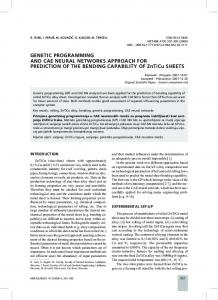
Fig. 1. Crossover in tree-based GP. Subtrees in parents are selected and exchanged.

2) Randomly select individuals from the population, and compare them with respect to their fitness. The fitness measure defines the problem the algorithm is expected to solve. 3) Modify fitter individuals using some or all of the following variation operations: • Reproduction—Copy an individual without change. • Recombination—Exchange substructures between two individuals. • Mutation—Exchange a unit in an individual at a random position. . 4) If the termination criterion is not reached, 5) Stop. The best individual represents the best solution found. A comparatively young and growing research area in the context of evolutionary algorithms is GP that uses computer programs as individuals. In early work, Friedberg [9], [10] attempted to solve simple problems by teaching a computer to write computer programs. Because of his choice of search strategy, however, he failed. Based on the success of EAs in the 1980s, Cramer applied an evolutionary algorithm to computer programs. Programs were already represented as variable-length tree structures in his TB language [7]. It was then with the seminal work of Koza [14], [15] that the field of GP really took off. In GP, the individual programs map-given input–output examples, called fitness cases, whereas their fitness depends on the mapping error. The inner nodes of the program trees are functions, and the leafs are terminals that mean input variables or constants. The operators applied to generate individual variants, i.e., recombination and mutation, must guarantee that no syntactically incorrect programs are allowed to be generated during evolution (syntactic closure). Fig. 1 illustrates the recombination operation in a tree-based GP system.

In recent years, the scope of GP has expanded considerably and now includes evolution of linear and graph representations of programs as well, in addition to tree representations [3]. A strong motivation for investigating different program representations in GP is that for each representation form as well as for different learning methods in general, problem domains exist that are more suitable than are others. A. Linear Genetic Programming In the experiments described below, we use linear GP, a GP approach with a linear representation of individuals. Its main characteristic in comparison to tree-based GP is that expressions of a functional programming language (like LISP) are substituted by programs of an imperative language (like C). The use of linear bit sequences in GP again goes back to Cramer and his JB language [7]. Cramer later discarded his approach in favor of a tree representation. A more general linear approach was introduced by Banzhaf [2]. Nordin’s idea of using machine code for evolution was the most radical “down-to-bones” approach [17] in this context. It was subsequently expanded [18] and led to the automatic induction of machine code by genetic programming (AIMGP) system [3], [20]. In AIMGP, individuals are manipulated directly as binary machine code in memory and are executed directly without passing an interpreter during fitness calculation. This results in a significant speedup compared with interpreting systems. Because of their dependence on specific processor architectures, however, AIMGP systems are restricted in portability. Our LGP system implements another variant of LGP. An individual program is represented as a variable-length string composed of simple C instructions. An excerpt of a linear genetic program is given as follows.

BRAMEIER AND BANZHAF: A COMPARISON OF LINEAR GENETIC PROGRAMMING AND NEURAL NETWORKS IN MEDICAL DATA MINING

Fig. 2.

19

Crossover in LGP. Continuous sequences of instructions are selected and exchanged between parents.

TABLE I INSTRUCTIONS IN LGP

{

} The instruction set (or function set) of the system is composed of arithmetic operations, conditional branches, and function calls. The general notation of each instruction type listed in Table I shows that—except for the branches—all instructions (destination implicitly include an assignment to a variable variable). This facilitates the use of multiple program outputs in LGP, whereas in tree-based GP those side effects need to be incorporated explicitly. Instructions either operate on two variables (operand variables) or on one variable and one integer constant . At the beginning of program execution, these variables hold the program inputs, and at the end, the program output(s). Variables and constants form the “terminal set” of LGP. Each instruction is encoded into a four-dimensional vector that holds the instruction identifier, indexes of all participating variables, and a constant is represented as value (optionally). For instance, . Because each vector component uses one byte of memory only, the maximum number of variables is restricted to 256 and constants range from 0 to 255 at maximum. This representation allows an efficient recombination of the programs as well as an efficient interpretation.

Partially defined operations and functions are protected by returning a constant value (here, 1) for all undefined inputs. Sequences of branches are interpreted as nested branches like in C that allows complex conditions to be evolved. If the condition of a branch or nested branch is false, only one instruction is skipped, namely, the next nonbranch in the program. This treatment of conditionals has enough expressive power because leaving out or executing a single instruction can deactivate much of the preceding effective code or reactivate preceding noneffective code, respectively (see Section II-B). The evolutionary algorithm of our GP system applies tournament selection and puts the lowest selection pressure on the individuals by allowing only two individuals to participate in a tournament. The loser of each tournament is replaced by a copy of the winner. In such a steady-state EA, the population size is always constant and determines the number of individuals created in one generation. Fig. 2 illustrates the two-point string crossover used in LGP for recombining two tournament winners. A segment of random position and random length is selected in each of the two parents and exchanged. If one of the resulting children would exceed the maximum length, crossover is aborted and restarted with exchanging equally sized segments. The crossover points only occur between instructions. Inside instructions, the mutation operation randomly replaces the instruction identifier, a variable, or the constant (if existent) by equivalents from valid ranges. Constants are modified through a certain standard deviation (mutation step size) from the current value. Exchanging a variable, however, can have an enormous effect on the program flow that might be the reason why in LGP, high mutation rates have been experienced to produce better results. In GP, the maximum size of the program is usually restricted to prevent programs from growing without bound. In our LGP system, the maximum number of instructions allowed per pro-

20

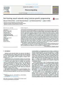
Fig. 3.

IEEE TRANSACTIONS ON EVOLUTIONARY COMPUTATION, VOL. 5, NO. 1, FEBRUARY 2001

Elimination of intron code (white) in LGP. Only effective code (black) is copied to the execution buffer.

gram has been set to 256. For all tested problems, this configuration has been experienced to be a sufficient maximum length. Nevertheless, individual programs of maximum length can still vary in size of their effective code (effective length; see Section II-B). Because each instruction is encoded into four bytes of memory, an individual holds at most 1 KB of memory. That makes the system memory efficient as well.

manipulating variables that are not used for the calculation of the outputs at that program position. In contrast to that, a semantical intron is an instruction or a sequence of instructions that manipulate relevant variables in which the state of the variables remains constant. Three rather simple examples of semantical introns are as follows: 1) 2)

B. Removing Introns at Runtime In nature, introns denote DNA segments in genes with information that is not expressed in proteins. The existence of introns in eucaryotic genomes may be explained in different ways: 1) because the information for one gene is often located on different exons (gene parts that are expressed), introns may help to reduce the number of destructive recombinations between chromosomes by simply reducing the probability that the recombination points will fall within an exon region [28]. In this way, complete protein segments encoded by specific exons are more frequently mixed than interrupted during evolution. 2) Perhaps even more important for understanding the evolution of higher organizms is the realization that new genetic material can be “tested” while retaining a copy of the original information in intron code. After the DNA is copied, the introns are removed from the resulting messenger-RNA that actually participates in gene expression, i.e., protein biosynthesis. A biological reason for the removal of introns might be that genes are more efficiently translated during protein biosynthesis in this way. Without being in conflict with ancient information held in introns, this might have an advantage, presumably through decoupling of DNA size from direct evolutionary pressure. In analogy, an intron in a genetic program is defined as a program part without any influence on the calculation of the output(s) for all possible inputs. Other intron definitions common in GP postulate this to be true only for the fitness cases [3], [19]. Introns in GP play a similar role as introns in nature in that they act as redundant code segments that protect advantageous building blocks from being destroyed by crossover. Further, they also contribute to the preservation of the diversity of the population by retaining genetic material from direct evolutionary pressure. Two types of introns can be distinguished in LGP. Structural introns denote single noneffective instructions that emerge from

3) Example (3) is a special case because the operation is not executed at all because of the condition of the branch, which is never fulfilled. Because it is much easier for the GP system to implement structural introns, the rate of semantical introns in linear genetic programs is usually low. In the following, the term “intron” always denotes a structural intron. The program structure in LGP allows introns to be detected and eliminated much easier than in tree-based GP. In LGP, all noneffective instructions are removed from a genetic program before evaluating fitness cases. This is done by copying all effective instructions to a temporary program buffer. This action does not affect the representation of the individuals in the population (see Fig. 3). Thus, the important property of the noneffective code to protect the information holding code from being disrupted is preserved. In analogy to the elimination of introns in nature, the linear genetic code is interpreted more efficiently. Because of this analogy, the term “intron” might be more justified here than in tree-based GP. The following algorithm detects all structural introns in a linear genetic program. Note that whether a branch is an intron only depends on the status of the operation that directly follows. In the example program from Section II-A, all instrucare introns, provided that the program tions marked with an and . outputs are stored in Algorithm 2 (Intron Detection): 1) Let the set always contain all program variables that have an influence on the final program output at the current position. is output variable Start at the last program instruction, and move backward. . 2) Mark the next operation with destination variable . If such an instruction is not found,

BRAMEIER AND BANZHAF: A COMPARISON OF LINEAR GENETIC PROGRAMMING AND NEURAL NETWORKS IN MEDICAL DATA MINING

21

TABLE II MEDICAL DIAGNOSIS TASKS OF PROBEN1 BENCHMARK DATA SETS

3) If the operation directly follows a branch or a sequence of branches, mark these instructions also; else, remove from . 4) Insert the operand variables of new marked instructions in if not already contained, . 5) Stop. All nonmarked instructions are introns. All marked instructions are copied to form the effective proat worst, where gram. The algorithm needs linear runtime is the maximum length of the genetic program. Actually, detecting and removing the noneffective code from a program only requires about the same time as calculating one fitness case. The more fitness cases that are calculated, the more this computational overhead will pay off. By ignoring noneffective instructions during fitness evaluation, a large amount of computation time can be saved. A good estimate of the overall acceleration in runtime is the factor (1) denotes the average intron percentage of a genetic where denotes the respective percentage of program and effective code. The intron percentage of all individuals is computed by this algorithm and can be put to further use, e.g., for statistical analysis. LGP programs can be transformed into functional expressions by a successive replacement of variables starting with the last effective instruction. It is obvious that such a tree would grow exponentially with effective program length and could become extremely large. These trees normally contain many identical subtrees, because the more they grow, the more instances of a variable are likely to be replaced by the next assignment. This might give an indication of what we believe is the expressive power of a linear representation. III. THE MEDICAL DATA SETS In this contribution, GP is applied to six medical problems. Table II gives a brief description of the diagnosis problems and the diseases that are to be predicted. Medical diagnosis problems always describe classification tasks that are much more frequent in medicine than approximation problems. The data sets have been taken unchanged from an existing collection of real-world benchmark problems, PROBEN1 [21], that was established originally for NNs. The results obtained with one of the fastest learning algorithms for feedforward NNs (RPROP) accompany the PROBEN1 benchmark set to serve as

TABLE III PROBLEM COMPLEXITY OF PROBEN1 MEDICAL DATA SETS

a direct comparison with other methods. Comparability and reproducibility of the results are facilitated by careful documentation of the experiments. Following the benchmarking idea, the results for NNs have been adopted completely from [21]. But most results have been verified by test simulations. The main objective of the project was to realize a fair comparison between GP and NNs in medical classification and diagnosis. We will show that for all problems discussed, the performance of GP in generalization comes close to or is even better than the results documented for NNs in [21]. All PROBEN1 data sets originate from the UCI Machine Learning Repository [5]. They are organized as a sequence of independent sample vectors divided into input and output values. For better comparability of results, the representation of the original (raw) data sets has been preprocessed in [21]. Values have been normalized, recoded, and completed. All inputs are restricted to the continuous range [0, 1], except for data set that holds or only. For the outputs, the a binary 1-of-m encoding is used in which each bit represents one of the -possible output classes of the problem definition. Only the correct output class carries a “1,” whereas all others carry “0.” It is characteristic for medical data that they suffer from unknown attributes. In PROBEN1, most of the UCI data sets with missing inputs have been completed by 0 (30% in data set). case of the Table III gives an overview of the specific complexity of each problem expressed in the number of attributes, divided into continuous and discrete inputs, plus output classes and number of samples. Note that some attributes have been encoded into more than one input value. IV. EXPERIMENTAL SETUP A. Genetic Programming For each data set, an experiment with 30 runs has been performed with LGP. Runs differ only in their choice of a random

22

IEEE TRANSACTIONS ON EVOLUTIONARY COMPUTATION, VOL. 5, NO. 1, FEBRUARY 2001

TABLE IV PARAMETER SETTINGS FOR LINEAR GP

seed. Table IV lists the common parameter settings used for all problems. For benchmarking, the partitioning of the data sets was adopted from PROBEN1. The training set always included the first 50% of the samples from the data set, the next 25% were defined as the validation set, and the last 25% were the test set. In PROBEN1, three different compositions of each data set were prepared, each with a different order of samples. This should increase the confidence that results are independent of the particular distribution into training, validation, and test set. The fitness of an individual program is always computed using the complete training set. After each generation, generalization performance is checked by calculating the error of the best-so-far individual using the validation set to check its ability during training. The test set is used only for the individual with minimum validation error after training. of an individual program Throughout this paper, fitness has two parts, the mean square error (MSE) and the classification error (CE). The MSE is calculated using the squared and the desired difference between the predicted output for all -training samples and -outputs. The mean output classification error (MCE) is computed as the average number of incorrectly classified examples

(2) The mean CE is weighted by a parameter (see Table IV). In this way, the classification performance of a program determines selection directly. The MSE allows additional continuous fitness improvements. For fair comparison, the winner-takes-all classification method has been adopted from [21]. Each output class corresponds to exactly one program output. The class with the highest output value designates the response according to the 1-of-m output representation introduced in Section III. Because only classification problems are dealt with in this contribution, the test classification error characterizing the generalization performance and the generation in which the indi-

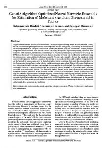
vidual with the minimum validation error appeared (effective training time) are the quantities of main interests. 1) Population Structure: In evolutionary algorithms, the population of individual solutions may be subdivided into multiple subpopulations. Migration of individuals among the subpopulations causes evolution to occur in the population as a whole. Wright first described this mechanism as the island model in biology [29] and reasoned that in semi-isolated subpopulations, called demes, evolution progresses faster than in a single population of equal size. This inherent acceleration of evolution by demes could be confirmed for evolutionary algorithms [27] and for GP in particular [26], [1]. One reason for this acceleration may be that genetic diversity is preserved better in multiple demes with restricted migration. Diversity in turn influences the probability that the evolutionary search hits a local minimum. A local minimum in one deme might be overcome by other demes with better search direction. A nearly linear acceleration can be achieved in evolutionary algorithms if demes are run in parallel on multiprocessor architectures [1], [6]. A special form of the island model, the stepping-stone model [13], assumes that migration of individuals is only possible between certain adjacent demes that are organized as graphs with fixed connecting links. Individuals can reach remote populations only after passing through these neighbors. In this way, the possibility that there will be an exchange of individuals between two demes depends on their distance in the graph topology. Common topologies are ring or matrix structures. In our experiments, the population is subdivided into ten demes, each holding 500 individuals. This partitioning has been found to be sufficient for investigating the effect of multiple demes. The demes are connected by a directed ring of migration links by which every deme has exactly one successor (see Fig. 4). After each generation, a certain percentage of best individuals from each deme, determined by the migration rate, emigrates into the successor deme, thereby replacing the worst individuals. By reproducing locally best solutions into several demes of the population, learning may accelerate because these individuals might further develop simultaneously in different demes. Care has to be taken, however, against premature loss of diversity caused by a faster proliferation of

BRAMEIER AND BANZHAF: A COMPARISON OF LINEAR GENETIC PROGRAMMING AND NEURAL NETWORKS IN MEDICAL DATA MINING

PERCENTAGE

OF INTRONS,

TABLE V EFFECTIVE CODE, AND BRANCHES PER RUN WITH SPEED-UP FACTORS FOR REMOVING INTRONS PROGRAM EXECUTION. NOTABLE DIFFERENCES EXIST BETWEEN PROBLEMS

Fig. 4. Stepping-stone model of directed migration on a ring of demes.

best individuals in the population. Specifically, if the migration between demes is not restricted to certain migration paths or occurs too frequently, this might happen. Therefore, migration between demes has been organized in a ring topology here with a modest migration rate of about 5%. B. Neural Networks Experimental results in [21] have been achieved using standard multilayer perceptrons (MLPs) with fully connected layers. A different number of hidden units and hidden layers (one or two) had been tried before arriving at the best network architecture for each data set. The training method was RPROP learning [22], a fast and robust backpropagation variant. For further information on the RPROP parameter settings and the special network architectures, the reader may consult [21]. The generalization performance on the test set was computed for the state of the network with minimum validation error during training. The number of epochs, i.e., the number of times the training samples were presented to the network, until this state was reached measures the effective training time of the network. V. RESULTS AND COMPARISON A. Intron Rate Table V shows the average percentage of noneffective code and effective code per run (in percent of the absolute program length) as well as the resulting acceleration [using (1)] for the medical problems under consideration. Regularly, an intron rate of 80% has been observed that corresponds to an average decrease in runtime by intron elimination of about a factor 5. This

23

BEFORE

speedup is of practical significance, especially when operating with large data sets as they occur in medicine. A further benefit of removing noneffective code is that the higher processing speed of the genetic programs would make them more efficient in time-critical problem environments. We emphasize again that the elimination of introns as described in Section II-B cannot have any influence on the fitness or classification performance of a program. From Table V, it can also be observed that the percentages strongly vary with the problem. The differences in results between the three data sets tested for each problem were found to be only tiny and are, therefore, not specified here. The standard deviation of runs has proven to be amazingly small by comparison. For some problems, including , , and , the best classification results (see below) have been produced without conditional branches. This might be because if branches are not necessary for a good solution, they will promote rather , have specialized solutions. Other problems, especially worked considerably better with branches. Except for branch instructions, all problems have been tried with the same function set and system configuration. Compared with other operations and function calls, branches are cheap in execution time. Additional computation is saved with branches because not all (conditional) operations of a program are executed for each training sample. The average percentage of branches in a linear genetic program is given in Table V for the benchmark problems solved with branches. In general, the calculation of the relative speedup factors relies on the assumption that different instructions of the instruction set are homogeneously distributed in the population, including both noneffective code and effective code of the programs. B. Generalization Performance Table VI shows the classification error rates obtained with GP and NNs, respectively, for the medical data sets discussed in Section III. Best and average CE of all GP runs are documented on the validation and test set for each medical data set, together with the standard deviation. A comparison with the test CE of NNs (reprinted from [21]) is most interesting. For that purpose, the difference between the average test errors of NN and GP is printed in percent. Unfortunately, the classification results on the validation set and the results of the best runs are not specified in [21]. Our results demonstrate that LGP is able to reach a generalization performance similar to multilayer perceptrons using

24

IEEE TRANSACTIONS ON EVOLUTIONARY COMPUTATION, VOL. 5, NO. 1, FEBRUARY 2001

TABLE VI CLASSIFICATION ERROR RATES OF GP AND NN FOR PROBEN1 MEDICAL DATA SETS. NN DATA TAKEN FROM [21]. DIFFERENCE AVERAGE NN RESULTS. POSITIVE s INDICATE IMPROVED GP RESULTS OVER NN

1

RPROP learning. The small number of runs performed for each data set may, however, give an order of magnitude comparison only. In addition, the results for GP are not expected to rank among the best, because parameter settings have not been adjusted to each benchmark problem. This has deliberately not been carried out to show that even a common choice of the GP parameters can produce reasonable results. In contrast, the NN architecture applied in [21] has been adapted specifically for each data set. Finally, the PROBEN1 data sets, especially the coding of input and output values (see Section III), are prepared for being advantageous to NNs but not necessarily to GP approaches. problem, the test CE (average and Notably, for the standard deviation) has been found to be much better with GP. This is another indication that GP is able to handle a very high number of input dimensions efficiently (see Table III). On the turned out to be considerably more difficult other hand, for GP than for NN judged by the percentage difference in average test error. Looking closer, classification results for the three different data sets of each problem show that the difficulty of a problem may change significantly with the distribution of data into training, validation, and test set. Especially, the test error differs with the data distribution. For instance, the test error than for . For is much smaller for data set some data sets, the training, validation, and test sets cover the data space differently. As a result, a strong difference between and validation and test error might occur, as in the examples discussed above. C. Training Time The effective training time specifies the number of (effective) generations or epochs, respectively, until the minimum validation error occured. We can deduce from Tables III and VII that

1 IN PERCENT FROM BASELINE

TABLE VII EFFECTIVE TRAINING TIME OF GP AND NN (ROUNDED)

more complex problems cause more difficulty for GP and NN and, thus, a longer effective training time. A comparison between generations and epochs is, admittedly, difficult, but it is interesting to observe that effective training time for GP shows lower variation than for NN. Another important result of our GP experiments is that effective training time can be reduced considerably by using demes (as described in Section IV), without leading to a decrease in generalization performance. A comparable series of runs without demes but with the same population size has been performed for the first data set of each problem. The average

BRAMEIER AND BANZHAF: A COMPARISON OF LINEAR GENETIC PROGRAMMING AND NEURAL NETWORKS IN MEDICAL DATA MINING

TABLE VIII CE RATES OF GP WITHOUT DEMES. AVERAGE RESULTS SIMILAR TO RESULTS WITH DEMES (SEE TABLE VI)

25

in size and free from redundant information. Thus, the elimination of noneffective code in our LGP system serves another purpose in generating more intelligible results than do NNs. VI. DISCUSSION AND FUTURE WORK

TABLE IX EFFECTIVE TRAINING TIME OF GP WITH AND WITHOUT DEMES. SIGNIFICANT ACCELERATION WITH DEMES

classification rates documented in Table VIII differ only slightly from the results obtained with a demetic population (see Table VI). Table IX compares the effective training time using a panmictic (nondemetic) population with the respective results from Table VII after the same maximum number of 250 generations. On average, the number of effective generations is reduced by a factor of about three when using demes. Thus, a significantly faster convergence of the runs is achieved with a demetic approach. This acceleration may be because of the elitist migration strategy applied here. D. Further Comparison Reducing the (relative) training time on a generational basis also affects the absolute training time, because runs may be stopped earlier. Comparing the absolute runtime in GP and NNs, the fast NN learning algorithm has been found to be superior. We should keep in mind, however, that large populations have been used with the GP runs to guarantee sufficient diversity and a sufficient number of demes. Moreover, because we concentrated on a comparison in classification performance, the configuration of our LGP system has not been optimized for runtime. If a small population size would be used, intron elimination that accelerates LGP runs several times will help to relax the difference in runtime between both techniques. In contrast to NNs, GP is not only capable of predicting outcomes, but it may also provide insight into and a better understanding of the medical diagnosis by allowing an analysis of the resulting genetic programs [16]. Knowledge extraction from genetic programs is more feasible with programs that are compact

We have reported on LGP applied to a number of medical classification tasks. All data sets originate from a set of realworld benchmark problems established for NNs [21]. For GP, a standard set of benchmark problems still does not exist. Such a set would give researchers the opportunity for a better comparability of their published methods and results. An appropriate benchmark set should be composed of real-world data sets taken from real problem domains as well as artificial problems in which the characteristics of the data are exactly known. But a set of benchmark problems is not enough to guarantee comparability and reproducibility of results. A parameter that is not published or an ambiguous description can make an experiment irreproducible and may lead to erratic results. In many published contributions, either comparisons with other methods were not given at all or experiments with the methods compared to had to be reimplemented first. In order to make a direct comparison of published results easier, a set of benchmarking conventions has to be defined, along with the benchmark problems. These conventions should describe standard ways of setting up and documenting an experiment, as well as measuring and documenting the results. A step in this direction has been taken by Prechelt for NNs [21]. We have presented an efficient algorithm for the detection of noneffective instructions in linear genetic programs. The elimination of these introns before fitness evaluations results in a significant decrease in runtime. In addition, the number of relevant generations of the evolutionary algorithm was reduced by using a demetic population in tandem with an elitist migration strategy. Increasing the runtime performance of GP with these techniques is especially important when operating with large data sets from real-world domains like medicine. By using demes in GP, we observed that the best generalization on the validation set is reached long before the final generation. Wasted training time can be saved if runs are stopped earlier. However, appropriate stopping rules that monitor the progress in fitness and generalization over a period of generations need to be defined. Information about the effective size of the genetic programs could be used for parsimony pressure. In contrast to punishing absolute size, this would not counteract intron growth. Rather, introns may fulfill their function as a protection device against destructive crossover operations, whereas programs with short effective code still would be favored by evolution. REFERENCES [1] D. Andre and J. R. Koza, “Parallel genetic programming: A scalable implementation using the transputer network architecture,” in Advances in Genetic Programming 2, P. J. Angeline and K. E. Kinnear, Eds. Cambridge, MA: MIT Press, 1996, pp. 317–337. [2] W. Banzhaf, “Genetic programming for pedestrians,” in Proc. 5th Int. Conf. Genetic Algorithms, vol. 628, 1993. [3] Genetic Programming—An Introduction. On the Automatic Evolution of Computer Programs and Its Application, 1998.

26

IEEE TRANSACTIONS ON EVOLUTIONARY COMPUTATION, VOL. 5, NO. 1, FEBRUARY 2001

[4] W. G. Baxt, “Applications of artificial neural networks to clinical medicine,” Lancet, vol. 346, pp. 1135–1138, 1995. [5] C. Blake, E. Keogh, and C. J. Merz. (1998) UCI repository of machine learning databases. Dept. Inform. Comput. Sci., Univ. California, Irvine, CA. [Online]. Available: [http://www.ics.uci.edu/~mlearn/MLRepository.html] [6] M. Brameier, F. Hoffmann, P. Nordin, W. Banzhaf, and F. D. Francone, “Parallel machine code genetic programming,” in Proc. Int. Conf. Genetic Evolutionary Computation, 1999. [7] N. L. Cramer, “A representation for the adaptive generation of simple sequential programs,” in Proc. 1st Int. Conf. Genetic Algorithms, 1985, pp. 183–187. [8] L. J. Fogel, A. J. Owens, and M. J. Walsh, Artificial Intelligence through Simulated Evolution. New York: Wiley, 1966. [9] R. Friedberg, “A learning machine—Part I,” IBM J. Res. Develop., vol. 2, pp. 2–13, 1958. [10] R. Friedberg, B. Dunham, and J. North, “A learning machine, part II,” IBM J. Res. Develop., vol. 3, pp. 282–287, 1959. [11] H. F. Gray, R. J. Maxwell, I. Martinez-Perez, C. Arus, and S. Cerdan, “Genetic programming for classification of brain tumours from nuclear magnetic resonance biopsy spectra,” in Genetic Programming 1996: Proc. 1st Annu. Conf., 1996. [12] J. Holland, Adaption in Natural and Artificial Systems. Ann Arbor, MI: Univ. Michigan Press, 1975. [13] M. Kimura and G. H. Weiss, “The stepping stone model of population structure and the decrease of genetic correlation with distance,” Genetics, vol. 49, pp. 313–326, 1964. [14] J. R. Koza, “Hierarchical genetic algorithms operating on populations of computer programs,” in Proc. 11th Int. Joint Conf. Artificial Intelligence, 1989, pp. 768–774. , Genetic Programming. Cambridge, MA: MIT Press, 1992. [15] [16] P. S. Ngan, M. L. Wong, K. S. Leung, and J. C. Y. Cheng, “Using grammar based genetic programming for data mining of medical knowledge,” in Genetic Programming 1998: Proc. 3rd Annu. Conf., 1998. [17] P. Nordin, “A compiling genetic programming system that directly manipulates the machine-code,” in Advances in Genetic Programming, K. E. Kinnear, Ed. Cambridge, MA: MIT Press, 1994, pp. 311–331. [18] P. Nordin and W. Banzhaf, “Evolving turing-complete programs for a register machine with self-modifying code,” in Proc. 6th Int. Conf. Genetic Algorithms, 1995, pp. 318–325. [19] P. Nordin, F. Francone, and W. Banzhaf, “Explicitly defined introns and destructive crossover in genetic programming,” in Advances in Genetic Programming II, P. Angeline and K. Kinnear, Eds. Cambridge, MA: MIT Press, 1996, pp. 111–134. [20] P. J. Nordin, “Evolutionary program induction of binary machine code and its applications,” Ph.D. dissertation, Dept. Comput. Sci., Univ. Dortmund, 1997. [21] L. Prechelt, “PROBEN1—A set of neural network benchmark problems and benchmarking rules,” Tech. Rep. 21/94, Univ. Karlsruhe, Karlsruhe, Germany, 1994.

[22] M. Riedmiller and H. Braun, “A direct adaptive method for faster backpropagation learning: The RPROP algorithm,” in Proc. IEEE Int. Conf. Neural Networks, San Francisco, CA, 1993, pp. 586–591. [23] B. D. Ripley and R. M. Ripley, “Neural networks as statistical methods in survival analysis,” in Artificial Neural Networks: Prospects for Medicine, R. Dybowski and V. Grant, Eds. Texas: Landes Biosciences, 1997. [24] H.-P. Schwefel, Evolution and Optimum Seeking. New York: Wiley, 1995. [25] R. L. Somorjai, A. E. Nikulin, N. Pizzi, D. Jackson, G. Scarth, B. Dolenko, H. Gordon, P. Russell, C. L. Lean, L. Delbridge, C. E. Mountford, and I. C. P. Smith, “Computerized consensus diagnosis—A classification strategy for the robust analysis of MR spectra. 1. Application to H-1 spectra of thyroid neoplasma,” Magn. Reson. Med., vol. 33, pp. 257–263, 1995. [26] W. A. Tackett, “Recombination, selection and the genetic construction of computer programs,” Ph.D. dissertation, Dept. Elect. Eng. Syst., Univ. Southern California, Los Angeles, 1994. [27] R. Tanese, “Distributed genetic algorithms,” in Proc. 3rd Int. Conf. Genetic Algorithms, 1989, pp. 434–439. [28] J. D. Watson, N. H. Hopkins, J. W. Roberts, J. A. Steitz, and A. M. Weiner, Molecular Biology of the Gene. New York: Benjamin/Cummings, 1987. [29] S. Wright, “Isolation by distance,” Genetics, vol. 28, pp. 114–138, 1943.

Markus Brameier was born in Witten, Germany, in August 1970. He received the diploma degree in computer science from the University of Dortmund, Germany, in 1997. He is currently working toward the Ph.D. degree in computer science at the same university. He is currently with the Chair of Systems Analysis, Department of Computer Science, University of Dortmund. Since 1997, he has been working on the Collaborative Research Center SFB 531 “Design and Management of Complex Technical Processes and Systems by Means of Computational Intelligence Methods” (sponsored by the Deutsche Forschungsgemeinschaft [DFG]). His current research interests include genetic programming and neural networks.

Wolfgang Banzhaf received the Ph.D. degree in physics. He has been an Associate Professor of Applied Computer Science at the University of Dortmund, Germany, since 1993. He was with the University of Stuttgart, Germany, where he conducted research on computers and synergetics. He was also a Senior Researcher at the Mitsubishi Electric Research Laboratories, Cambridge, MA, and a Member of the Neurocomputing Group, Mitsubishi Electric Central Research Laboratory, Japan. His current research interests include artificial neural networks, evolutionary algorithms, genetic programming and artificial life, and self-organization.