85
Optimising farm resource allocation to maximise profit using a new generation integrated whole farm planning model J. M. RENDEL1, A.D. MACKAY2, A. MANDERSON2 and K. O’NEILL1 1 AgResearch, Private Bag 50034, Mosgiel 2 AgResearch, Private Bag 11008, Palmerston North
[email protected]
Abstract
A new generation integrated whole farm planning model (“the model”) is introduced. In a departure from the use of whole farm and average data for decision making, this model integrates data from multiple land management units (LMUs) within a farm business and uses optimisation to identify farm system design to maximise profit under variable production and market conditions. The user supplies pasture growth rates, minimum and maximum acceptable pasture covers for each LMU, animal performance, farm costs and market prices. Additions or constraints can be placed on individual LMUs. The optimisation routine uses this information to identify the mix of production enterprises and management regimes that maximises profit for the business. A case study is presented based on a commercial sheep and beef farm with five distinct LMUs. Comparisons are made between: treating the farm as a single LMU and as five LMUs; with current and optimal farm system. Keywords: Farm System modelling, linear programming, optimisation, land management units, investment
Introduction
There is a need for a model that “paints a picture” of how an individual farm system may alter when changes are being considered (i.e., a strategic model, output of which could be used to inform existing monitoring models). This is made more challenging by the fact that most farms are an amalgam of diverse landscapes on which a diversity of changes could be made with varying results. These changes could include: additional fertiliser, new pasture species (e.g., lucerne, chicory, and Italian ryegrass), the effect of genetic gain in animals, drainage, irrigation, a new winter crop, or industry (regulatory) policy change. Any change firstly needs to be considered in a financial context and then may assist in understanding environmental implications (e.g., excluding cattle from a particular area of the farm over winter). Wider industry or local
and national government regulatory changes may also be factored into the model to understand their on-farm implications. This analysis then provides data which can be used to assess the value or cost to the farm owner of making investments or policy change which alter the resources available on farm. This paper describes and reports on the development and initial testing on a commercial sheep and beef farm of version I of the model.
Method and materials
A farm resource allocation model, which is a combination of a feed budget, stock reconciliation and financial budget, has been developed. The model is set up using linear programming (Pannell 1997), a mathematical technique that has previously been successfully applied in farm systems modelling (Feola et al. 2012). The model optimises the use of farm resources (land which is used for pasture and crop production; and sheep, cattle, including dairy grazers, and deer) whilst maximising profit. The land can be split into any number of land management units (LMUs) which are contiguous (or near contiguous) areas of the farm which have similar characteristics (e.g. pasture growth rate, slope, soil characteristics, etc.). The feed budget for each LMU and the overall stock reconciliation are the constraints, and the financial budget the objective function. The model maximises profit, while balancing the feed budget and reconciling livestock numbers. The year is split into 26 fortnightly periods. LMUs can have restrictions applied to management options e.g., cattle grazing in winter, cultivation, making of supplementary feed. The number of deer LMUs are specified (these can be zero). Animals can be moved between LMUs at the end of each period. Pasture covers at the beginning of the year must equal pasture covers at the end of the year, so as to prevent pasture mining (steady state). The model currently uses a single year. The objective (financial budget) does include costs associated with running animals which are allocated to the species and the class (ewes, cows, lambs, replacements, etc.) of stock. These costs include
86
Proceedings of the New Zealand Grassland Association 75:
labour, animal health, fuel and vehicle expenses, etc. The objective function also includes the costs of cropping, making and feeding out supplementary feed, transferring animals between LMUs (a per head cost that is currently the same for any movement between LMUs, however this will be allowed to vary between LMUs in a future version). The income from store stock sales (at weaning) and prime animal sales (animals for finishing are split into their sex mobs at weaning and these are then split into five equal sized groups based on liveweight) are included. The model includes fortnightly meat schedule which is based on carcass weight and GR. This allows the model to value animals fortnightly and then select when to sell. The objective function is whole farm EBITDA (Earnings before interest tax depreciation and amortisation) without the enterprise and land costs. This is referred to as rEBITDA (r for restricted). Note that the objective does not include costs that are related to running the enterprise (e.g., communication) or costs associated with the land (e.g., repairs and maintenance, rates, fertiliser) as these are not related to animal production and hence are fixed costs (do not vary with animal production or enterprise). The inputs (Table 1) and outputs (Table 2) to the model are similar to other farm system models. Animal details along with pasture details are used to estimate feed requirements (sheep and cattle requirements are estimated using GrazPlan equations (Freer et al. 2012); deer feed requirements using Dryden (2011) and NRC (2007)), as well as finishing and cull animal values. Future versions will include: the options to purchase store animals and strategically apply nitrogen; link the underlying land resource information with local climate to estimate pasture and crop growth and response to inputs. It would also be possible to optimise over multiple years, which would give indications of how a farm system may alter with seasonal variation. Case Study sheep and beef farm A case study farm was chosen to help validate the model, and to check it was making sensible decisions. It was also chosen to allow a comparison between modelling a farm that has multiple LMUs as a single LMU farm. The case study farm was a sheep breeding and finishing operation with beef cows and some cattle finishing. The farm covers 558 ha with landscapes that vary from flat and easy rolling to easy hill and a small amount of steepland (Table 3 and Figure 1). The farm costs were obtained from the 2012 Ministry of Primary Industries Farm Monitoring report for Central North Island Hill Country Sheep and Beef (Ministry of Primary Industries 2012). These were split into animal costs (included animal health, labour, breeding, etc.), land cost (rates, fertiliser, lime, etc.) and enterprise costs (accountancy,
85-90
(2013)
legal, etc.). The animal costs were allocated to sheep and cattle. For sheep, the wool revenues were deducted from the animal costs. Sheep were assumed to require 10% more labour per head than cattle, and cattle had a 50% higher animal health cost than sheep on a per head basis. Supplementary feed costs and cropping costs were not included in these calculations as they are options considered by the model. Other details on the farm operation are summarised in Table 4. The benefit of separating the farm into individual LMUs was explored by comparing the fully optimised system (i.e., all five LMUs) with that of optimising the farm as a single land unit, by using weighted (by LMU area) average pasture growth rates and energy contents (Figure 1) for the single unit. Then the farm system identified as being the most profitable by the model (fully optimised) was compared with the current farm system. The current system was modelled, as both pasture and animal growth rates are likely to be estimates. This was done by setting cow numbers at 9 September to at least 165, and ewe numbers also on 9 September to at least 3300. Also 10 ha of winter crop was planted in LMU1 (yield 9.1 t DM/ ha with 10.8 MJME/kg DM at a cost of $950/ha, planted mid-November). The model was run to provide stock numbers and rEBITDA.
Results and Discussion
Modelling the farm with multiple land management units The optimal livestock policy for the farm operating with five LMUs or as a single LMU was similar, with ewe numbers (Figure 2a) very similar (5260 and 5224 respectively). The total prime lambs (Figure 2b) and number of replacements (Figure 2c) were also very similar (the single LMU values are nearly the same as the total numbers for five LMUs, so were not graphed). The average pasture covers (Figure 2d) were almost the same as the average of the five LMUs weighted by area. The EBITDA was also very similar ($404 000 for the single LMU and $407 500 for five LMUs). The stocking rate, at 1 July, of was 13.7 SU/ha (where a ewe is 1.22 SU, and a ewe hogget is 1.0 SU). The benefit in separating the farm into five LMUs is that the stock locations can be shown. Figures 2(a), 2(b) and 2(c) show the locations of different classes of sheep over the year. Over the period from 2 weeks prior to lambing to weaning (where ewes are set stocked within LMU) there are small movements in two-tooths. From weaning until mating the two-tooths are on LMU 1 and 3. From January until lambing most ewes are on LMU 2 and 3 with LMU 4 being used by ewes from mid-March to mid-May. LMU 1, from January to mid-July, is used mostly to feed replacement ewe lambs and prime lambs. A small number of ewes are on LMU 1 over that time as well.
Optimising farm resource allocation to maximise profit... (J. M. Rendel, A.D. Mackay, A. Manderson and K. O’Neill)
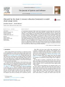
(a) Figure 1
(b)
Average fortnightly (a) pasture growth rates and (b) pasture quality for each land management unit (LMU).
A major advantage of having a picture of stock numbers is that it becomes relatively easy to visualise the effect of a change to farm resources on the farm system. What would the farm system look like if LMU 5 was put into lucerne or chicory, or LMU 3 was put into trees? We also get an estimate of EBITDA which helps in deciding the value of that technology to this particular farm system. Table 1
87
Another advantage is that of being able to visualise the effect of a restriction on the farm system. If cattle are in the model, there may be some areas of the farm that these should not be run due to environmental constraints or local government policy – we can see the impact of this on the farm system and on EBITDA. Optimised current and fully optimised farm system
Inputs required for the model
Farm
Area of each LMU Number of deer LMUs Latitude of farm
Pasture (for each LMU and each fortnight)
Pasture growth rate Pasture energy content Minimum and maximum permissible pasture covers Pasture utilisation by the animals
Crop (for each LMU where a crop can be planted)
Planting date First possible grazing date Last possible First grazing date of new grass
Supplementary feed
LMUs on which supplementary feed can be made Cost of making and feeding out Price received for sale Maximum percentage of an animal’s fortnightly intake that can come from supplementary feed
Animal (for each species)
Weights and growth rates (fortnightly) Scanning and weaning percentages Animal deaths Parturition and weaning dates Cull dates Replacement rate
Financial
Annual per animal costs Meat schedules Store stock prices Cost of transferring animals between LMUs Dairy Grazer agistment price
88
Proceedings of the New Zealand Grassland Association 75:
(d)
(c)
Table 2
(2013)
(b)
(a)
Figure 2.
85-90
(a) Ewe numbers, (b) finishing lamb numbers, (c) ewe replacement numbers, and (d) pasture covers on each of the five land management units (LMUs) and farmed as a single LMU.
Outputs from the model
Pasture (for each LMU and each fortnight)
Pasture cover at the end of the fortnight
Crop (for each LMU where a crop can be planted)
Area planted Amount fed each fortnight
Supplementary feed
For each LMU the fortnightly period and amount of supplementary feed made, transferred to other LMUs, fed and sold
Animal (for each species)
The number of each class of stock present at the end of each period on each LMU The number of sales, price and liveweight at the end of each fortnight The number of transfers to other LMUs at the end of each period The period and number of culls Daily feed requirements
Financial
rEBITDA
Optimising farm resource allocation to maximise profit... (J. M. Rendel, A.D. Mackay, A. Manderson and K. O’Neill)
The optimised current farm system had the same lamb sale dates as the fully optimised system (Table 5). Whereas the optimised current farm system sold most of the cattle store at weaning, with a small number being sold in June and July as R2yrs, the fully optimised farm system did not run cattle, instead wintered an additional 846 ewes. The optimised current system had EBITDA (calculated as rEBITDA less per hectare costs of $230/ ha and enterprise costs of $10 557) 5.1% less than the optimal system. Further, capital invested in livestock (using the 2013 IRD National Average Market Values) as at 30 June was 9.9% greater ($64 630) than the optimal system. The optimised current farm system had similar average pasture covers to the fully optimised system with the exception of November, when pasture covers are expected to be higher in the current farm system. However there were differences in covers on individual LMUs between the two systems, especially between April and July. The finding that the livestock numbers in the optimised current farm system (stocking Table 3
Area and annual pasture production of each LMU
LMU
Area (ha)
Pasture Grown (kg DM/ha/year)
1
208.7
12,133
2
178.6
9,323
3
50.2
5,733
4
89.8
7,353
5
30.7
12,133
Total
558.0
9,889
Table 4
rate of 13.8 SU/ha) are much higher than the livestock numbers on the existing case farm (10.4 SU/ha) suggests either: assumed levels of pasture production and utilisation are over-stated; the farm operates suboptimally for other reasons (e.g., risk, uncertainty, farm owner’s goals); the model needs further refinement; or a combination of the above. These will be explored further as part of the on-going development of the model.
Summary
We have developed a tool, albeit in the early stages of development, which we can use to explore the contribution each LMU makes to the farm business and how best to use the mix of LMUs to maximise farm returns. A major advantage of the tool is it provides a picture of the contribution each LMU makes and just where the livestock are located on the farm during the year. Further, the optimisation routine in the tool creates the opportunity for the first time to estimate the expected returns from specific on-farm investments targeted at specific LMUs on the whole farm business. The impacts of industry or government policy change can also be investigated using the model through the optimisation of resource allocation from different land management units. We identified that the optimal livestock policy for the farm operating with five LMUs was similar to the single LMU, indicating the model architecture is able to aggregate data from the five individual LMUs to produce a whole farm report. With this architecture in place it is possible to explore the contribution of each LMU to business performance,
Key dates, animal performance and costs for the case farm. Beef Cattle
Sheep
Scan date
20 May
12 Jul
Scan Dry %
5%
5%
Scan % (foetuses / female pregnant)
100%
168%
Dry cull date
4 June
26 Jul
Parturition Date
30 Sep
16 Sep
Wean Date
12 Apr
16 Dec
Wean % (per female at parturition)
90%
140%
Wean Weight (kg)
240 (Bull), 230(Steer), 220(Heifer)
26 (average)
Cull Date
30 May
19 Feb
Mature female weight at parturition
515kg
57kg
Replacement Rate %
22%
22%
Mature female annual cost
$25
$25
Replacement female annual cost
$17
$7
Finishing animal annual cost
$17
$7
Death Rate mature female
5% pa
5% pa
replacements
5% pa
5% pa
5% pa
5% pa
165 cows
3300 ewes
finishing animals
Stock numbers
89
90
Table 5
Proceedings of the New Zealand Grassland Association 75:
Comparison of the current optimised with fully optimised farm system. Current optimised
Fully optimised
Ewes (30 June)
4412
5258
Replacements
1101
1207
Prime Sales (Total)
4670
5565
March
573
682
April
937
1117
May
1502
1791
June
1294
1543
July
363
432
Cows (30 June)
167
Replacements
37
Store Sales (Wean)
96
Prime Sales (R2yr) 18 June
7
16 July
7
Crop (ha)
10
rEBITDA
$516 233
$536 912
EBITDA
$386 789
$407 468
without the confounding influence of other system changes. We also identified large differences between the current system operated by the case farm and that produced by optimising the current system. This may be due to estimates of key inputs being over optimistic, or a conscious decision by the farmer to meet other objectives, or the model needing further refinement, or all of the above.
ACKNOWLEDGEMENTS
85-90
(2013)
Funding from Ministry of Business, Innovation and Employment, DairyNZ, Fonterra, Beef + Lamb New Zealand, DCANZ and DeerResearch; advice on farmer needs from Beef + Lamb New Zealand. David Stevens and other reviewers for their helpful comments.Robyn Dynes and Andy Bray for their foresight.
REFERENCES
Dryden, G.M. 2011. Quantitative nutrition of deer: energy, protein and water. Animal Production Science 51: 292-302. Feola, G.; Sattler, C.; Saysel, A.K. 2012. Simulation models in farming systems research: potential and challenges. p. 490. In: Farming systems research into the 21st century: The new dynamic. Eds. Darnhoffer, I.; Gibbon, D.; Dedieu, B. Springer, Dordrecht. Freer, M.; Moore, A.D.; Donnelly, J.J. 2012. The GRAZPLAN animal biology model for sheep and cattle and the GrazFeed decision tool. CSIRO Plant Industry Technical Paper May 2012 Ministry of Primary Industries 2012. Farm Monitoring Report 2012 – Pastoral Monitoring: Central North Island hill country sheep and beef. http://www.mpi. govt.nz/newsresources/publications?title=Farm%20 Monitoring%20 Report NRC 2007. Nutrient requirements of small ruminants: sheep, goats, cervids, and new world camelids. The National Academies Press Pannell, D.J. 1997. Introduction to practical linear programming. John Wiley & Sons, Inc., New York. 333 pp.