International Journal of Research in Engineering and Technology (IJRET) Vol. 2, No. 5, 2013 ISSN 2277 – 4378
A Comparison of Neural Network Models for Load Forecasting in Nigerian Power System Kehinde O. Alawode and Mojeed O. Oyedeji
forecasts with least forecasting error. Numerous statistical approaches have been applied to the problem of load forecasting. These approaches include time series, similar-day approach, and regression methods. However, these methods are basically linear models and load forecasting is a nonlinear approximation problem, that is, it does not obey superposition principle. Neural networks are essentially non-linear circuits that have the capability to do non-linear curve fitting. The outputs of an artificial neural network are some linear or non-linear mathematical function of its inputs. Neural networks are suitable for load forecasting because of their approximation ability for nonlinear mapping and generalization of the relationship between the sets of inputs and outputs. Several studies have been carried out on the applicability of neural networks to short-term load forecasting. Most of them usually focus mainly on 24-hour-ahead, one-hour-ahead or next day load forecasting. However, in the application of neural networks to short-term load forecasting, some network parameters need to be carefully selected. The selection of these parameters affects the quality of load forecast obtained and the performance of the network in general. This paper compares two artificial neural network models with varied network parameters using the actual load data obtained from National Control Center (NCC) of Nigeria’s power utility company, the Power Holding Company of Nigeria (PHCN). The performance parameters used for the comparison are the mean squared error (MSE), mean percentage error (MPE) and training time.
Abstract— System operations and planning is an important aspect of power system management. The effectiveness of power system planning, however, depends to a large extent on the accuracy of load forecast obtained by power system planners. Most studies focus on the applicability of neural networks to 24-hour-ahead, one-hour-ahead or next day peak load forecasting. In this paper, we compare the performance of two artificial neural network models: the feed-forward backpropagation and the recurrent neural networks in load forecasting for Nigeria’s power system. The load data used were obtained from National Control Center of the Power Holding Company of Nigeria. The performance parameters used for the comparison are the mean square error (MSE), mean percentage error (MPE) and training time. Keywords— ANNs, Load forecasting, Supervised, Feedforward networks, Recurrent networks. I. INTRODUCTION
D
EMAND forecasting is a study essential to any industry involved in the production of a good or service. In the electrical power industry, load forecasting plays an important role in system planning and effective operation of a power system. Forecasting the future trend in electricity demand is important for network planning, infrastructure development, economic dispatch, fuel scheduling and unit maintenance. Short-term load forecasting covers forecasting ranging from hours to weeks. These forecasts are often needed for day-byday economic operations of power generation plants. The accuracy of forecast obtained is however of utmost importance to a system planner. Reference [1] reported that a one percent increase in forecasting error of electricity demand resulted in a £10 million increase in operating costs in the British power system. A poor load forecast misleads planners and often results in wrong and expensive expansion plans. Equally, overestimating future electric loads may result in a redundant reserve of electric power. On the contrary, underestimation of loads causes failure in providing sufficient electric power [2]. Thus, the major objective of load forecasting is to obtain
II. ARTIFICIAL NEURAL NETWORKS An Artificial Neural Network (ANN) is an information processing paradigm inspired by the way biological nervous system, such as the brain processes information. ANN evolved in an experiment performed by McCulloch and Pitts to model bio-systems using nets of simple logical operations in 1943. The neural network structure is composed of highly interconnected processing elements (neurons) working in parallel to solve a specific problem. ANN models the nonlinear relationship between network inputs and corresponding targets and uses this information to predict future values of outputs for a given set of input values. The basic functional unit of an ANN is the artificial neuron. The neuron receives numerical inputs, processes it internally and produces an output. The processing of inputs is done in
Kehinde O. Alawode is a Lecturer with the Department of Electrical and Electronic Engineering, Osun State University, Osogbo, Nigeria (+234 8056483153; e-mail:
[email protected]). Mojeed O. Oyedeji graduated with a First Class B. Eng. degree in Electrical and Electronic Engineering from Osun State University, Osogbo, Nigeria. (e-mail:
[email protected]).
218
International Journal of Research in Engineering and Technology (IJRET) Vol. 2, No. 5, 2013 ISSN 2277 – 4378
two stages. The first stage involves the linear combination of the input values. The combination uses weights attributed to each connection, and a constant bias term. The strength of the connection between an input and a neuron is denoted by the value of the weight. The result of the linear combination is used as the argument of a non-linear activation function. The activation function refers to the network activation rule. It acts as a limiting function. A number of activation functions available for use in ANNs include step, logistic, tangenthyperbolic, linear and cosine functions etc. The output of the neuron can be mathematically formulated as p (1) Lˆ = f wi x i + b , i 1 = Where wi are the synaptic weights, x i represents the model
hybrid learning for real-time load forecasting in Turkey. The model indicated better results compared to that of a time series. In [8], an approach for short-term load forecasting using the multi-layered feed forward ANN-based model was presented. The work attempts to demonstrate neural networks ability to predict load with minimal input data. A supervised neural network model was used in [9] to forecast the load in the Nigerian power system. The study emphasized the need for the number of neurons in the hidden layer to be carefully chosen as too may neurons may lead to overspecialization and consequently, loss of generalizing capability. Reference [10] used a Bayesian Neural Network (BNN) approach to solve the short term load forecasting problem. The Bayesian model is a probabilistic model which considers a probability density function (PDF) over the weight space. This arrangement handles some of the uncertainties in the modelling, thus further development could increase the quality of the forecasting models. In this present work, two neural network models: the feedforward backpropagation and the Elman recurrent neural networks are used to solve the short-term load forecasting problem in the Nigerian power system.
∑
input vector, and b denotes the bias. There are three fundamental classes of artificial neural networks: the single-layer feed-forward network, multi-layer feed-forward network and recurrent networks. The single-layer and multi-layer networks are known as static networks while the recurrent networks are dynamic. The ability of the neural network to recognize functional relationship or pattern between input and target data is referred to as learning; the learning process is determined by the type of paradigms, rules and algorithms involved. During the learning process, the network adapts and adjusts its synaptic weights to reduce the approximation error. The performance of the ANN is usually influenced by the type of network architecture, learning algorithm, number of hidden layers and hidden layer neurons.
IV. METHODOLOGY A. Input Vector Configuration The ANN inputs that were considered include the time of the day, day type and associated historical load data. Numerical values were assigned to the day type and time as follows; Indexes of 1-7 were assigned to represent the day type from Sunday to Saturday respectively and 1-24 to represent the hour of the day. Historical load data obtained from the NCC of the PHCN was arranged based on the following: • Load of the previous hour, L(t-1) • Load of the same hour the previous day, L(t-24) • Load of the same hour of the same day in the previous week, L(t-168) • Load of the previous hour of same hour of the same day in the previous week, L(t-169) The corresponding target is the load of the hour to be predicted, L(t). Therefore one training example consists of six input elements and one corresponding target.
III. LITERATURE REVIEW This section presents previous studies that have been carried out on the applicability of neural networks to load forecasting. A three-layered feedback backpropagation (BP) algorithm trained by genetic algorithm (GA) for short-term load forecasting was used in [3]. The research aimed at improving BP based ANN model to eliminate the drawbacks and establish an optimal network structure for better forecast. The GA approach illustrated a superior representation and addressed some problems encountered by ordinary backpropagation models. In [4], the application of ANNs to long-term load forecasting was demonstrated. The model forecasted the annual peak demand of a Middle Eastern utility and repeated the process using a time-series approach. Reference [5] presented a multi-layer feed-forward neural network model to compare the forecasting accuracy of a timeseries and an ANN-based model. The study concluded that the ANN-based model gave better results. A feedback ANN-based model was used in [6] to predict the hourly energy consumption in buildings. The model used a non-linear optimized data window size and hidden layers which could seriously affect the forecasting accuracy. In their work on intelligent short-term load forecasting, [7] used Elman’s recurrent neural network model with integrated
B. Data Pre-processing Due to wrong measurements and other human errors, some out-of- range values were observed in the historical load data as obtained from the PHCN, hence the need to detect and replace such bad data. Bad data was detected by locating any value that is three standard deviations away from the mean of the whole distribution. These values were then replaced by the average of L(t-1), L(t-24) and L(t-168). Normalization of the data was also done to scale the inputs and targets by dividing the actual value by the maximum value. This has the effect of scaling the data within limits suited for the activation function to be used. It also improves interpretability of the network weights. 219
International Journal of Research in Engineering and Technology (IJRET) Vol. 2, No. 5, 2013 ISSN 2277 – 4378
TABLE I PERFORMANCE PARAMETERS FOR MODEL 1
C. Network Models In this paper, two ANN-based models developed using MATLAB are compared. Model 1 incorporates a feed-forward network architecture which carries out learning using a backpropagation algorithm that updates its weight and bias values based on Levenberg-Marquardt optimization. Model 2 uses the dynamic Elman recurrent network architecture which uses a network training function which updates its weight and bias values according to conjugate gradient backpropagation with Polak-Ribiére updates. Both network models use a tansigmoid activation function in the hidden layer(s) and a purelin function in the output layer. The number of hidden layer neurons for both networks was fixed at 20. However, the selection of the number of hidden layers to be used for the comparison was based on experiment. In each of the cases, the number of hidden layers was varied between 1 and 5 and the case with the best performance was selected. The pre-processed data was divided into both training and testing sets. Both network models were trained using data from the training set. The trained neural network models were subsequently simulated, firstly with data from the training set and secondly, with testing data which were not previously used in training. The simulation was performed using data covering a period of one week (168 hours). The load forecast obtained from the simulation was compared with the corresponding actual load data and the error is calculated. The MPE and MSE were used to evaluate the performance of these models and are defined by (2) and (3). These values were obtained using normalized load values. n (x − y 1 i i) (2) × 100 MPE = n i =1 xi
1 n
i
− yi ) 2
Training goal achieved (× 10-3)
1.47
Number of hidden layers 2 3 4 5 21.41 70.00 169.97 291.09
1.32
1.46
1.40
1.59
B. Forecasting Using Model2 Model2 was trained using 1200 training examples in the batch training mode. Table II presents the results from variation of the number of hidden layers. From the Table the case with the least training goal achieved is when the network is trained with three hidden layers, therefore the network performance was evaluated using this case. TABLE II PERFORMANCE PARAMETERS FOR MODEL 2
Performance Parameters Training time (s)
n
∑ (x
1 3.45
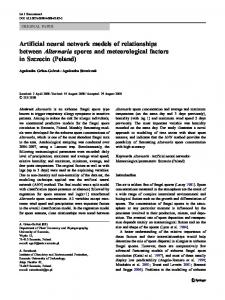
To evaluate the generalization capability of the network, its performance was evaluated again using another data set other than the training data set (testing set) over the same one week period. The MPE and MSE values recorded were 3.48 × 10⁻⁴ and 4.02 × 10⁻⁴ respectively. Fig. 1 (a) and (b) show the network response using training and testing data sets respectively, while Fig. 1(c) shows the error of approximation over the period of evaluation. The training set has minimum and maximum error values of -282.66 and 235.62 respectively. The testing set has minimum and maximum error values of 344.12 and 206.03 respectively. This shows this the network model has a very good generalization capability.
∑
MSE =
Performance Parameters Training time (s)
(3)
i =1
Training goal achieved (× 10-3)
V. RESULTS In this section, the results obtained using the feed-forward and the recurrent neural network models for forecasting the power system load are presented and discussed.
2 1315.12 1.11
Number of hidden layers 3 4 5 2287.61 8594.51 12569.50 0.86
0.93
1.31
The MPE and MSE values obtained over a period of 168 hours using the training data set are 2.21 × 10⁻³ and 3.85 × 10⁻⁴ respectively. The generalization capability of the network was also evaluated by simulating the network with the testing data sets. The MPE and MSE values recorded for this simulation were 4.64 × 10⁻³ and 4.98 × 10⁻⁴ respectively. The performance plots for the Elman neural network is shown in Fig. 2. In the training set, the approximation error ranges from -216.82 to 222.55, while in the testing set, the error ranges between -345.25 and 289.45. This shows that the generalization capability of the network model is very good.
A. Forecasting Using Model1 Model1 was trained using 12000 training examples in the batch training mode. Table 1 presents the results obtained from training the network with varied number of hidden layers. From Table 1, it can be observed that the training time increases with the number of hidden layers. However with two hidden layers, the network has the least mean square error (indicating the best training goal achieved), thus the case of the two hidden layers was used for the comparison. The network performance was evaluated using data from the training set over a period of 168 hours. The MPE and MSE values obtained were 5.06 × 10⁻⁴ and 3.42 × 10⁻⁴ respectively.
220
International Journal of Research in Engineering and Technology (IJRET) Vol. 2, No. 5, 2013 ISSN 2277 – 4378
Performance Plot - Using Training Data 3600
Performance Plot - Using Training Data Actual Load Forecasted Load
3600 Actual Load Forecasted Load
3400
3400
3200
Load (MW)
Load (MW)
3200
3000
3000
2800
2800
2600
2600
2400
24
48
72
96
120
144
168
2400
Time (Hours)
24
48
72
96
Time (Hours)
120
144
168
(a)
(a)
Performance Plot - Using Testing Data 3600 Actual Load Forecasted Load
Performance Plot - Using Testing Data 3600
3400
Actual Load Forecasted Load 3400
3200
3000
Load (MW)
Load (MW)
3200
2800
3000
2800
2600
2600
2400
24
48
72
96
120
144
168
Time (Hours) 2400
(b)
24
48
72
96
120
144
168
Time (Hours) (b)
Error Plot 400
Error Plot
Training Set Testing Set
300
Actual Error (MW)
Actual Error (MW)
Training Set Testing Set
-400
24
48
72 96 Time (Hours)
120
144
-400
168
24
48
72
96
120
144
168
Time (Hours)
(c) (c)
Fig. 1 Performance plots for feed-forward neural network model
Fig. 2 Performance plots for Elman recurrent neural network model
221
International Journal of Research in Engineering and Technology (IJRET) Vol. 2, No. 5, 2013 ISSN 2277 – 4378
VI. CONCLUSION The results from the training and simulation of the two network models show that the Elman recurrent network provided better load forecast due to its relative low error of forecast when compared with the feed-forward backpropagation model. However, the feed-forward model is best suited for incorporation in real-time load forecasting systems due to its least training time which implies fast response. This paper has also shown that increasing the number of hidden layers does not necessarily improve the network performance but rather it increases the training time. REFERENCES [1]
D.W. Bunn and E.D Farmer. Comparative Models for Electrical Load Forecasting, John Wiley and Sons, New York, 1985, p. 232. [2] P. Pai, “Hybrid ellipsoidal fuzzy systems in forecasting regional electricity loads” Energy Conversion and Management, Volume 47, Issues 15-16, September 2006, pp. 2283-2289 [3] D. Srinivasan. “Evolving artificial neural networks for short-term load forecasting”, Neuro-computing, Volume 23, Issues 13, December 1998, pp. 265-276 [4] T. Al-Saba and I. El-Amin . “Artificial neural networks as applied to long-term forecasting, AI in Engineering, 1999, pp. 189-197, [5] S.S. Sharif and J.H Taylor. “Short-term Load Forecasting by Feed Forward Neural Networks”, Proc. IEEE ASME First Internal Energy Conference (IEC), Al Ain, United Arab Emirate, 2000. [6] A.P. Ganzalez and J.M. Zamarreno. “Prediction of hourly energy consumption in building based on a feedback artificial Network”. Energy and Buildings, Volume 37, Issue 6, June 2005, pp. 595-601. [7] I. Erkme, A.K. Topalli and I. Topalli. “Intelligent short-term load forecasting in Turkey” International Journal of Electrical Power & Energy Systems, Volume 28, Issue 7, September 2006, pp. 437-447 [8] S. Georges, N. Kandil, M. Saad and R.Wamkeue. “An efficient approach for short-term load forecasting using neural network” International Journal of Electrical Power & Energy Systems, Volume 28, Issue 8, October 2006, pp. 525-530 [9] G.A. Adepoju, K.O. Alawode, and S.O.A. Ogunjuyigbe. “Application of Neural Network to Load Forecasting in Nigerian Electrical Power System” The Pacific Journal of Science and Technology, Volume 8, Number 1, May 2007, pp. 68-72. [10] E. Fock, P. Lauret, J. Manicom- Ramsamy, R.N. Randrianarivony (2007) “Bayesian neural network approach to short time load forecasting” Energy Conversion and Management, Volume 49, Issue 5, May 2008, pp. 1156-1166.
222