A comparison of Neural and Graphical Models for Syntactic and Structural Pattern Recognition Terry Caelli and Walter F. Bischof Department of Computing Science University of Alberta, Canada tcaelli,
[email protected]
Mario Ferraro Dipartimento di Fisica Sperimentale University of Turin, Italy
[email protected]
Abstract Recent developments in the theory and uses of Bayesian Networks in pattern recognition and image understanding (PRIU) raise questions about the relationships between Bayesian compared to non-Bayesian approaches. In this paper we compare Neural-based verses Bayesian-based methods for PRIU. We conclude with the view that a singular PRIU architecture that models “from pixels to predicates” in one explicit system model, is most desirable from an optimization perspective and that hierarchical hidden Markov random fields are one example of such an approach but where algorithms from neural computing also apply.
1. Introduction Pattern recognition and Image Understanding (PRIU) models are differentiated by their data structures and algorithms. and over the past decade or so, a number of PR models have evolved to address the limitations of standard PR classifier methods. These include: 1. Modular and model-based neural networks 2. Graph matching 3. Relational rule learning - conditional rule generation 4. Graphical models - Bayesian nets, hidden Markov random fields In this paper we discuss similarities and differences between these approaches and point to how experience with them all is leading to new insights about a unified theory of syntactic and structural PR for complex signal understanding. Figure 1 attempts to organize current PRIU problems in terms of the richness of the data models and types of algorithms used. The first cluster of models have input data structures that can very from pure attributes (as with statistical pattern recognition and normal feedforward neural nets, for example) to labeled, attributed vertices of
Data Model Statistical pattern classifiers Model-based Neural Nets
a1
c1
an
cm
f1
g1
fn
gm
Graph Matching
Relational Learners Bayesian Networks
Numerical Optimization Least Squares Gradient Descent Levenberg-Marquardt,etc.
S1 O1
Algorithms
Sn On
Probabilistic Optimization Dynamic Programming Probabistic Relaxation Expectation-Maximization Markov Chain Monte Carlo Tree search
Figure 1.
Neural, statistical and recent graph matching approaches to PRIU perform interpretation by solving optimization problems in terms of minimizing errors between mappings of the model onto data using numerical optimization methods. Bayesian methods solve the same optimization problem by usually having a more explicit minimum description length data model, MAP (maximum a posterior probability) image labeling criteria and probabilistic optimization methods. Here a, c, f, g, s, o refer to attributes, classes, input functions, output functions, states (labels) and observations respectively.
graphs (as occurs in Model-based Neural Nets and Graph matching). Outputs vary from classes, labels to labeled and attributed vertices as well - for graph matching. In all these cases, however, the estimation problem is typically that of determining a single transformation from input to output data structures using techniques from numerical optimization. For example in graph matching, the aim is to determine the least squares approximation to the permutation matrix that maps one set of graph vertices into another [21]. That is, this class of methods typically solve PRIU via global optimization procedures although depending on the degree of decomposition, model-based Neural Nets do allow for global solutions with explicit subprocess constraints. The second cluster of models (Bayesian Networks, Relational Learners) assume an explicit relational data model where the inputs and outputs are generally defined as attributed and labeled nodes vertices all within
the same network flow model. The states of each node are inferred from other state and/or observation nodes and dependencies are defined by contingency (conditional probability) tables for Bayes Nets and relational learners (for example, Conditional Rule Generation (CRG) [7]). What particularly differentiates this second cluster of models from the first is the nature of what is being optimized and how it is being performed. Such models typically attempt to determine the optimal state at each node, given the model and observations and no particular distinction is made between “input” and “output”. For example, in image annotation, a hierarchical hidden Markov Random Field model is used to determine the optimal labels at each pixel, feature or region given the model and observations [5, 11]. As a consequence of this, the derivation of optimal states over the graphical model is determined by quite different algorithms including dynamic programming, probabilistic relaxation labeling Expectation-Maximization, through to a range of sampling methods including Markov Chain Monte Carlo [14]. In the following we provide some illustrate examples of these different approaches and point to benefits and deficits of the approaches.
2. Model-Based Neural Networks Although traditional statistical and neural-based PR is not relational over the past years there has been a good deal of research in using neural architectures for solving a wide range of problems including graph matching and relational learning. This is basically accomplished by defining input nodes in terms of functions or pre-identified (labeled) graph nodes having observable attributes and matching (this form of PR) reduces to determining the mapping of input labeled nodes to the output nodes and so determining the correspondences [20]. This illustrates how a neural net model actually provides another type of approximation to the permutation matrix that minimizes the mapping between the vertices of two attributed graphs as recently studied by [21]. In general, a neural net can be defined as a directed graph [16] whose nodes (neurons) are characterized by input-output functions with connections between pairs of nodes (i, j) characterized by a weight matrix W ≡ wij . Tree-like neural net topologies are commonly used in pattern recognition [3], even though recurrent network, such as Boltzmann Machines have also been used for classifying image features [15]. In practice, however, constraints must be imposed for the net to work properly, and this is particularly true in the case of PRIU where the dimensionality of the input space is very high and would require a large number of neurons to carry out even simple tasks. Prior information on the nature of the perceptual problem is defined by the distribution p(W ), and this result in the presence of a
regularizing term in the error function, XX µ 2 E (wij ) = (Oi − tµi ) + P (W ), i
(1)
µ
where P is the regularization term. For instance, it is often assumed that the weight values must be limited, and this leads to p(w = Z exp(−λ/2w2 )), where λ is a parameter and Z constant. This, in turn, leads Pa normalizing 2 to P = λ/2 ij wij the well known weight decay regulerizer. Analogous to the role of priors in Bayesian methods, here such constraints improve the ability of generalization of the net since it makes it less dependent on the training set. Alternatively, one can attain minimization of the error function by using variational techniques and deriving the activation functions as Green functions of the operator P : this leads to a Gaussian form for the output y and to the well known Radial Basis Function Networks [3], [19]. That is such prior information is used to guide the search procedure being encoded in the net in an implicit way via the the error function and are aimed at guaranteeing specific characteristics of the encoding and recognition/matching scheme. It is clear that specific problems require specific weight models for the net to carry out the desired task. For instance, most traditional approaches to pattern recognition lack explicit shift, rotation, and scale invariance. Considering again in invariant pattern recognition a well known solution to the problem is via the so called P sigmapi units [3], in which the linear relation hi = j wij xj is replaced by sum of products of the inputs, and where the weights are made to depend on these specific relation between input coordinates to ensure that the net respond to the transformed pattern T f (x) in the same way as to the original pattern f (x): h(T f ) = h(f ). A more general approach is provided by the theory of Model Based Neural Networks (MBNN) [9, 12, 8] that aims to include more specific constraints on the network geometry and weights. MBNN have the feed-forward architecture of perceptrons, but they are buit specifically to respond to features in the data that are known a priori, to characterize the task or to have desired invariance, rather than hoping that the training data will produce, via the optimization techniques, the optimal set of weights. To this aim, in MBNNs input-ouput realizations, weights and activation functions all are subject to modeling via constraints which control the search procedures or guide the information flow through the network in such a way to guarantee given solutions. In MBNNs weight are parameterized and their values can be made to depend on the position in the net. Nodal distances are thus defined [9] to parametrically structure information processing in terms of the relative position of the neuron within each layer such that neurons in different positions perform different operations on the input. Weights are of the form wij = w (a, dij ) ,
(2)
where a is a vector of weights. In general the dimension of a can be kept less the number of weights, so reducing the space in which the search for the solution takes place. Also, in Model-based Neural Networks, activation functions are not restricted to a bounded monotonic functions of the input, such as the logistic function or the hyperbolic tangent, but can be any function, whose form is determined by the problem to be solved. The use of specialized units with given activation functions provides a significant simplification of the net and allows for complex computations without an excessive computational load. Note, however, that MBNNs remain in the general framework of perceptron models since every specific functional form of such specialized units is equivalent to the output of a network of the traditional type. Any continuous function can be approximated, up to a given precision, by a perceptron with just one layer of hidden neurons with activation functions φi (hi ). That is, the continuous function, f , is approximated via a linear combination N M X X wij xj , (3) α i φi f (x1 · · · xn ) = i=i
j=1
where φi are logistic. The problem is how many hidden units are necessary? In general it seems that their number grows exponentially with the number of input units, xj . Thus, although any specialized units with given activation function f could be represented by a multilayered perceptron the computation load would be typically significant. The freedom in the choice of activation functions makes it possible to build specialized units that can be connected to form more complex nets making the MBNN modular. Networks for solving complex problems can be formed by considering a set of simple nets Ni performing computations in parallel such that the output of Ni is the input of Nj , j > i for every i; thus for instance, N1 ∪ N 2 → N 3 ,
(4)
denotes two nets N1 , N2 working in parallel and whose outputs are inputs to a third net N3 [8]. Advantages of modularitiy has been discussed in several works (see for instance (for a review see [8], or [15]). Since it decomposes complex task in simpler one in modular networks speed of learning is increased, since complex task are and also the representation of the input data developed by a modular network tends to be easier to understand than in the case of ordinary NN. Thus, it can be said that MBNN replace the generic implicit constraints used in traditional NN with explicit representations of the form the desired solution must take, this reduces the computational load of the network but, perhaps more importantly, improves its generalization capabilities, since important features of the solution do not depend on the training data.
MBNN has been proved successful to perform pattern recognition tasks [9] and, and more generally, to carry out algebraic calculations, differential operations and computations of geometrical entities of the theory of surfaces (first and second fundamental forms, Gaussian and mean curvatures) [12]. Finally, the concatenations of subnets into complex structures enables MBNN to perform many task that usually require some symbolic form of processing, thus showing that NN are not necessarily “subsymbolic” and that the distinction between connectionist and symbolic approaches to knowledge representation has become somehow blurred. In all, then, over the past decade or so it has become clear the neural computing models for pattern recognition are quite capable of performing all types of classification and matching problems at numerical, structural and symbolic levels. However, common to all neural computing models is the use of either perceptrons or nonlinear normalizers (including probability-types) and casting the processing models in terms of a singular network architecture where inputs, outputs and processing units all share common properties. As will be seen, the main difference between neural computing models and Bayesian networks is how the estimation and prediction problems are solved since neural computing algorithms mainly employ numerical optimization methods compared to those derived from sampling and, more generally, probabilistic models.
2.1 Conditional Rule Generation Analogous to the encoding and matching graphs or structures using model-based and modular neural networks piece-wise decomposition and inductive learning approaches to PRIU have recently been developed using rule-based methods [6]. These methods combine the advantages of numerical learning methods with those of relational learners by induction over numerical attributes constrained by relational pattern models. Conditional Rule Generation (CRG), generates rules that take the form of numerical decision trees that are linked together so that relational constraints of the data are satisfied. Generation of a rule tree proceeds is illustrated in Figure 2). Once CRG has generated rules from training samples, the problem of recognition reduces to part labeling with respect to different models and their parts. Again, the very purpose of the CRG method has been to pre-compile the types of part and relational attribute states that are necessary and sufficient for recognition. Fortunately this can be accomplished by a direct activation of the CRG rules in a parallel, iterative deepening method. Starting from each scene part, all possible sequences of parts, termed chains, are generated and classified using the CRG rules. CRG generates classification rules for spatial (and spatio-temporal [1, 2]) patterns involving a small number of pattern parts subject to the fol-
1 2 3
U
4 5 6
UB3
8−7 8−10 8−9 11−8 8−11 UB31
1−2 UB32 UB2
7 9
8 11
Figure 2.
8
10 UBU21
evidence vectors. This compatibility measure can be characterized as follows. For a chain Si of parts pi1 , pi2 , . . . , pin , the compatibility of evidence vectors is defined as
U3 U2 5 1 11 3 6 8 7 9 10 2 4 U1
3−2 9−8 6−5 5−6 7−8 10−8 UB21 UB22
5 6 UBU211
2 UBU212
Example of input data and conditional decision
tree generated by CRG method. The left panel shows input data and the attributed relational structures generated for these data, where each vertex is described by a unary feature vector u ~ and each edge by a binary feature vector ~b. The right panel shows a cluster tree generated for the data on the left. Numbers refer to the vertices in the relational structures, rectangles indicate generated clusters, grey ones are unique, white one contain elements of multiple classes. Classification rules of the form Ui − Bij − Uj . . . are derived directly from this tree.
lowing constraints: 1) The pattern fragments involve only pattern parts that are adjacent in space (and time), 2) the pattern fragments involve only non-cyclic chains of parts, 3) temporal links are followed in the forward direction only to produce causal classification rules that can be used in classification and in prediction mode. A set of classification rules is applied to pattern in the following way. Starting from each pattern part (at any time point), all possible chains (sequences) of parts are generated using parallel, iterative deepening, subject to the constraints the only adjacent parts are involved and no loops are generated. Note that spatio-temporal adjacency and temporal monotonicity constraints were also used for rule generation. Each chain S is classified using the classification rules, and the evidence vectors of all rules instantiated by S are averaged to obtain the evidence ~ vector E(S) of the chain S. Further, the evidence vectors of all chains starting at a part p is averaged to obtain an initial evidence vector for p. Evidence combination using simple averaging is adequate only if it is known that a single pattern is to be recognized. However, if the test pattern consists of multiple patterns then this simple scheme can easily produce incorrect results because some some part chains may not be contained completely within a single pattern. These chains are likely to be classified in a arbitrary way, and to the extent that they can be detected and eliminated, part classifications can be improved. We use general heuristics for detecting rule instantiations [2] involving parts belonging to different patterns. They are based on measuring the compatibility of part evidence vectors and chain
n
w(S ~ i) =
1X~ E(pik ) n
(5)
k=1
~ ik ) refers to the evidence vector of part pik . where E(p This can be initially found by averaging the evidence vectors of the chains which begin with part pik . Then the compatibility measure can be used for updating the part evidence vectors in an iterative relaxation scheme: X 1 ~ (t+1) (p) = Φ ~ , E w ~ (t) (S) ⊗ E(S) (6) Z S∈Sp
where Φ P is the logistic function, Z a normalizing factor Z = S∈Sp w(t) (S), and where the binary operator ⊗ is defined as a component-wise vector multiplication [a b]T ⊗ [c d]T = [ac bc]T . The updated part evidence vectors then reflect the partitioning of the test pattern into distinct subparts. Figure 3 shows an example of how relational structural rules are generated from 3D objects for tolerancing. (a) Training with segmented views/samples of different models. Each label corresponds to model attributed parts
View 1
4
View 2 a
2
1
c
3 5
b
d
f
e
(c) Model Projection by rule instantiation. Typical model rule B(a,b)
(b) Generate Model Description rules: lists of parts, relations and their attributes (focal features/datum):If {part i has these attributes (U(i)) AND has these relations to part j (B(i,j)) AND part j has these attributes..etc..} then {evidence for model x is y}
(d) Tolerancing Process
B(3,4)
U(b)
U(a) U(c)
U(4)
U(3) DEFECT No instantiation in known rules
Figure 3. Example of the CRG method for industrial tolerancing: finding correspondences between model features to identify product deformations.
Such learning and recognition methods can be compared with MBNN in so far as different rules, more or less, could correspond to different sub-modules of a MBNN. However, since these rules are derived using principles of Minimum Description Length(MDL) and information reduction [2], the algorithms differ significantly than those used in neural computing. The benefits of CRG over MBNN lie in the expressibility of the rules,
the induction procedure and the simplicity of the rule instantiation procedures. Of particular importance is the induction procedure that essentially performs a relational hashing in the form of “rule graphs” [17].
2.2 Hierarchical hidden Markov random fields Both MBNNs and CRG can be formulated, in Bayesian terms, as specific types of network decomposition models in the form:
random field (MRF). In this model (see Figure 4), each layer l consists of two random fields to encode the hidden labeling process (X l ) and the observed image (Y l ). The ith node (pixel) for the hidden and observation random fields are denoted by xli and yil , respectively. Since the posterior (label) probability at any given layer l, p(X l |Y l ), is computational intractable we introduce further assumptions which enable us to perform model parameter estimation in a feasible way. These are:
1. In any given layer l, the observed random field Y l is solely depended on the hidden states at the same p(a1 , .., an , b1 , ..bm ) = p(b1 /a1 )p(a1 /a2 , ..ar )..p(bm /ai , ..).. level, X l : (7) p(Y l |X ALL , Y ALL ) = p(Y l |X l ) (8) where ~a, ~b correspond to input and output structures (attributes, labels, etc.) respectively. In this sense, then, where X ALL , Y ALL refer to the complete labelboth representations and algorithms can be replaced by ing/observation hierarchy. Further, each observed Bayesian Nets and the use of probabilistic learning (f0r data pixel is dependent only on its corresponding example Expectation-Maximization), exact or inexact instate (label): ference methods (for example, Loopy Belief Progagation) Y for classification and matching [18]. p(Y l |X l ) = p(yil |xli ). (9) What is missing, however, in these models is an asi sociated topology that permits a simplification of choices of possible connections and a single transparent model 2. The intra-layer hidden states are only dependent on for progressing from “pixels-to-predicates”. Hierarchitheir adjacent layers, i.e.: cal (multiscaled) Markov Random Fields(HHMRF) prop(X l |X ALL) = p(X l |X ∂l ) (10) vide such a topology and associated algorithms including Dynamic Programming and Expectation Maximizawhere X ALL refers to the whole hidden hierarchy, tion (EM) [4, 5]. The model we discuss here is closest, but and X ∂l corresponds to the neighborhood layers of not identical to, that of Cheng et. al. [10] using supervised X l , i.e., X l−1 , and X l+1 . learning to help estimate the important features within and between observation and label hierarchies. The ba3. In each layer l, the inter-layer hidden states (labels) sic mode is shown in Figure 4. What differentiate this are independent of each other, that is: approach from the others is that it incorporates a form of Y p(X l |Y l ) = (11) p(xli |yil ). hierarchical constraint propagation using bijective operai tors (short range and long support kernels) and the tuning of the model parameters to best fit expert annotation and Consequently, the hierarchical hidden Markov tree the use of colour images. (HHMT) encodes image content or structure (Figure 4) by: 3 3
Y
X
X
Y
2
1
X
2
1
Y
Figure 4.
The basic hierarchical hidden Markov tree (HHMT) model. Here only three levels (l − 1, l,l + 1) of the multiscale representation are shown. At each level there are two random fields corresponding to observed pixels, Y, image region labels defined by X. The bijection operations shown in grey and black colors (with corresponding arrows) represent upward and downward support kernel operators and associated region label transitions over movements upwards and downwards in scale, encapsulating two types of contextual constraints: long-range (downward) and short-range(upward).
The observed image Y is a random field sampled from an underlying stochastic process X, which is a Markov
− λ = {(πl , A+ l−1,l , Al,l−1 , Bl ); l = 1, .., L}
(12)
where the upward state transition matrices A+ are defined by: ˆ (l−1) = ~i). (13) A+ (~i, j) = p(x(l) = j/∂s l−1,l
s
The downward transition matrices A− are defined by: (l)
(l−1) ˆ ~ = j/∂s A− l,l−1 (i, j) = p(xs
= ~i).
(14)
ˆ (l+1) = ~i defines its contextual For position j in layer l, ∂s ˆ (l−1) = ~j corresponds to parents (clique, kernel), and ∂s its contextual children. In both cases, these kernels are defined by indexed histogram (see below). For each layer the prior probabilities of each label is defined by: πil = p(X l = i).
(15)
the relative frequencies of expected image labels at a given scale, l. The observation matrices B l are defined by B ≡ {B l , l ∈ [1..L]}, where B l (o, c) ∈ B l characterize the likelihood of the observed pixel values (o) at level l, given label c ∈ [1..C], which are selected from a set of Gaussian mixtures in the label-dependent cluster space and correspond, after normalization, to
Once the model is extracted any image can be interpreted with respect to the model by simply running the model on the new image until it converges. An example of this is shown in Figure 5 and demonstrates how, over iterations, even with similar images, the HHMT enables differential image classification (maximum posterior probability (MAP) score differences), segmentation and interpretation of image structure all within a single process. As can be seen the HHMRF’s are an explicit relational model for PRIU in so far as all model components and identified and modeled. This is comparable to MBNNs and relational learners although the learning, estimation and matching algorithms differ being formally Bayesian in nature. Albeit, the HHMRF algorithms are only approximations to the exact estimation problem and, as such, fall into local minima as do relaxation and nonexact least squares models used in neural computing.
3
(d)
(b)
(e)
(16)
(c)
Similarity Scores
B l (o, c) = p(y l = o/xl = c).
(a)
Using Sim ilarity Scores for Forestry Image Segm entation/Recognition -11500 -13500 -15500
1
2
3
4
5
Image (a)
-14444
-13613
-13616
-13616
-13616
Image (d)
-15452
-14715
-14718
-14721
-14720
Conclusions
Perhaps, then, the greatest difference between recent Bayesian Network models for PRIU (as illustrated here with HHMRFs) is the use of single highly constrained graphical models whose topology is designed to enable the development of complete PRIU systems in one single explicit architecture and set of learning, classification and matching algorithms. This explicit form, and associated MAP formulation, makes clearer how the different optimization techniques apply in contrast to the more “hidden” states view of neural computing - excluding MBNNs. However, the issues of appropriate priors, the inexact estimation and inference methods used in Bayesian models do not necessarily place such probabilistic models as provably superior to neural-based on rule-based approaches. What Bayesian methods do offer is a rich expressive representational language for PRIU modeling and the formulation of what is to be optimized and regularized typically in MAP terms and without assuming a single gaussian model as, for example, is the case with least squares formulations. Such Bayesian approaches has already been demonstrated to be successful in other areas of computer vision including stereo and basic image segmentation [13]. Such results, and the initial type of model described here, suggest that Bayesian models may well be a fertile unifying language for PRIU that enables
(f)
Num ber of Iterations
Figure 5. The HHMT model was estimated using image (a) and tested on images (a) and (d). We have used 4 classes corresponding to Aspen, Spruce, Shadows (both the shadow on the trees and on the ground) and Ground. Labeling results are shown using different colours. (b) and (e) show labeling after the first iteration (i.e., Naive Bayes Classifier) while (c) and (f) after five iterations. The bottom graph (g) shows the similarity scores (average log MAP probabilities per image) for the image data given the model as a function of the number of iterations of the algorithm.
us to incorporate past experience with model-based neural nets, relational learning. What is still an open question issue is the discovery of truly optimal algorithms for learning, inference, classification and matching.
References [1] W. F. Bischof and T. Caelli. Learning structural descriptions of patterns: A new technique for conditional clustering and rule generation. Pattern Recognition, 27:689–698, 1994. [2] W. F. Bischof and T. Caelli. Learning complex action patterns with crgst. In S. Singh, N. Murshed, and W. Kropatsch, editors, Advances in Pattern Recognition IACPR 2001, pages 280–289. Springer, Berlin, 2001.
[3] C. M. Bishop. Neural Networks for Pattern Recognition. Clarendon Press, Oxford, UK, 1995. [4] C. Bouman and B. Liu. Multiple resolution segmentation of textured images. IEEE Transactions on Pattern Analysis and Machine Intelligence, PAMI-13(2):99–113, 1991. [5] C. Bouman and M. Shapiro. A multiscale random field model for bayesian image segmentation. IP, 3(2):162– 177, March 1994. [6] T. Caelli and W. Bischof. Machine Learning and Image Interpretation. Plenum Books, 1997. [7] T. Caelli and W. F. Bischof, editors. Machine Learning and Image Interpretation. Plenum, New York, NY, 1997. [8] T. Caelli, L. Guan, and W. Wen. Modularity in neural computing. Proceedings of the IEEE, 87(9):1497–1518, 1999. [9] T. Caelli, D. Squire, and T. Wild. Model-based neural networks. Neural Networks, 6:613–625, 1993. [10] H. Cheng and C. A. Bouman. Multiscale bayesian segmentation using a trainable context model. IEEE Transactions on Image Processing, 10:51–525, 2001. [11] L. Cheng, T. Caelli, and V. Ochoa. A trainable hierarchical hidden markov tree model for color image segmentation and labeling. In ICPR 2002, pages 192–195, Quebec city, Canada, 2002. IEEE Press. [12] M. Ferraro and T. Caelli. Neural computations of algebraic and geometrical structures. Neural Networks, 11:699–707, 1998. [13] D. Forsyth and J. Ponce. Computer Vision: A Modern Approach. Prentice Hall, 2002. [14] W. Gilks, S. Richardson, and D. Spiegelhalter, editors. Markov Chain Monte Carlo in Practice. CRC Press, New York, NY, 1995. [15] S. Haykin. Neural Networks. A Comprehensive Introduction. Prentice-Hall International, London, UK, 1994. [16] B. Muller, R. Reinardt, and M. Strickland. Neural Networks. Springer-Verlag, Berlin, 1995. [17] A. Pearce, T. Caelli, and W. Bischof. Rulegraphs for graph matching and pattern recognition. Pattern Recognition, 27:1231–1248, 1994. [18] J. Pearl. Probabilistic Reasoning in Intelligent Systems: Networks of Plausible Inference. Morgan Kaufmann Publishers, San Mateo, California, 1988. [19] T. Poggio and F. Girosi. Networks for approximation and learning. Proceedings of the IEEE, 78:1481–1497, 1997. [20] P. Suganthan, E. Teoh, and D. Mital. Pattern recognition by grpah matching using the potts mft neural networks. Pattern Recognition, 28:997–1009, 1995. [21] A. van Wyk, T. Tariq, and B. van Wyk. A rkhs interpolator-based graph matching algorithm. IEEE Transactions on Pattern Analysis and Machine Intelligence, 24(7):988–995, 2002.