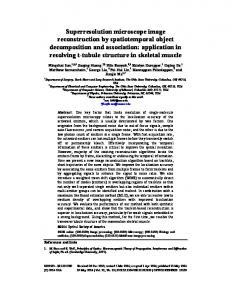
A comparison of superresolution reconstruction methods for multiangle CHRIS/Proba images Jonathan Cheung-Wai Chan∗, Jianglin Ma, Frank Canters Cartography & GIS Research Group, Department of Geography, Vrije Universiteit Brussel, Pleinlaan 2, 1050 Brussels, Belgium ABSTRACT Compact High Resolution Imaging Spectrometer onboard the Project for On-board Autonomy, or CHRIS/Proba, represents a new generation of satellite images that provide different acquisitions of the same scene at five different angles. Given the hyperspectral-oriented waveband configuration of the CHRIS images, the scope of its application would be much wider if the present 17m nadir resolution could be refined. This paper presents the results of three superresolution methods applied to multiangular CHRIS/Proba data. The CHRIS images were preprocessed and then calibrated into reflectance using the method described in [1][2]. Automatic registration using an intensity variation approach described in [3] was implemented for motion estimation. Three methods, namely non-uniform interpolation and de-convolution [4], iterative back-projection [5], and total variation [6] are examined. Quantitative measures including peak signal to noise ratio [7], structural similarity [8], and edge stability [9], are used for the evaluation of the image quality. To further examine the benefit of multi-frame superresolution methods, a single-frame superresolution method of bicubic resampling was also applied. Our results show that a high resolution image derived from superresolution methods enhance spatial resolution and provides substantially more image details. The spectral profiles of selected land covers before and after the application of superresolution show negligible differences, hinting the use of superresolution algorithm would not degrade the capability of the data set for classification. Among the three methods, total variation gives the best performance in all quantitative measures. Visual inspections find good results with total variation and iterative back-projection approaches. The use of superresolution algorithms, however, is complex as there are many parameters. In this paper, most of the parameter settings were tuned manually or decided empirically. Keywords: CHRIS/Proba, hyperspectral, superresolution, non-uniform interpolation and de-convolution, iterative backprojection, total variation
1. INTRODUCTION Hyperspectral remote sensing images are effective in many application domains where conventional broadband multispectral imagery finds its limits. For examples, in a study of mapping detailed ecotopes, hyperspectral images are 10% higher in overall accuracy compared to simulated Landsat images [10]. Hyperspectral analyses in urban land cover types draw similar conclusions. In a detail study on spectrometry for urban area [11], Herold et al. concluded that current multispectral systems such as IKONOS and Landsat ETM+ only provide marginal ability to resolve the separation of important urban land features. Despite the comparative advantages of hyperspectral images for land cover mapping in both rural and urban areas, their use for operational mappings remains limited. One reason is that the availability of hyperspectral data at high resolutions is still scarce. Though airborne hyperspectral acquisitions provide very fine resolution data, its use for large-scale mapping, at national or continental scales for examples, is not practical not just because of cost, but also because of technical issues concerning data consistency. Comparing with spaceborne data, airborne acquisitions are less flexible in regular revisiting, and the mosaicking of airborne data are often not straightforward due to distortions in spectral properties at the edge of the scans. Hence, for the mapping of large areal coverage, satellite images are still a preferred option. Among the more well-known spaceborne hyperspectral-oriented data is CHRIS/Proba which provides multiple observations of the same scene at five different angles (+55, +36, 0, -36, 55). The mode 3 (land channel) acquisition consists of 18 bands between 0.4-1μm. Its multiple acquisitions can be used as inputs for superresolution image reconstruction which is a technique to produce a high resolution (HR) image from several low resolution (LR) images [12]. Superresolution methods have been applied to remote sensing images such as ∗
[email protected]; phone +32 2629 3556; fax +32 2629 3378
Landsat [13][14], SPOT [15], Quickbird [14], multi-looking thermal data [16], as well as hyperspectral data [17]. Most of the previous studies are based on multitemporal data. To date there is no work on SR’s application on CHRIS/Proba images. In this paper, we present the latest results of applying different SR methods on CHRIS/Proba images. The objective is to further our understanding of a high resolution CHRIS image derived from conventional SR methods. Quantitative indices as well as visual assessments are used to evaluate the SR image results. The pros and cons of the conventional methods are also discussed.
2. SUPERRESOLUTION METHODS SR techniques are closely related to the problems of image restoration and image interpolation. The purpose of image restoration is to recover a degraded image without changing the dimension of the image. Based on similar theories as image restoration, SR can be considered as a second generation of image restoration techniques which also change image dimension. Image interpolation techniques can be used to increase the size of an image. However, the quality of a single LR image is limited and interpolation based on an undersampled image does not allow recovering the lost highfrequency information. Hence multiple observations of the same scene are needed. Superresolution refers to the reconstruction methods that can be applied to obtain an image with higher spatial resolution through the use of several lower-resolution (LR) images. The main objective is to achieve the best image quality possible from several LR images. However, not all LR images are useful for SR. The application of SR algorithms is possible only if aliases exist, and the images have sub-pixel shifts. There are many different SR techniques and they can be applied in the frequency domain or the spatial domain. However, the latter provides better flexibility in modeling noise and degradation, we focus our analysis in the spatial domain [18]. Conventional spatial domain methods include the nonuniform interpolation approach, the regularization reconstruction approach, the projection onto convex sets approach, hybrid approaches and others [12]. SR can also be applied on a single-frame LR image [19], which is more commonly referred to as image scaling, interpolation, zooming and enlargement. An important step in SR is to provide a model of the relationship between the original high resolution image and a set of LR images of the same scene. If we have p LR images, then the relationship between the LR images yk and the HR image X can be formulated as follows: yk = Dk Ck Fk X + nk , for 1 ≤ k ≤ p or ⎡ y1 ⎤ ⎡ D1C1F1 ⎤ ⎡ n1 ⎤ ⎢ ⎥ ⎢ ⎥ ⎢ ⎥ ⎢ ⎥=⎢ ⎥X + ⎢ ⎥ ⎢ y p ⎥ ⎢ D p C p Fp ⎥ ⎢n p ⎥ ⎣ ⎦ ⎣ ⎦ ⎣ ⎦
(1)
(2)
where y k stands for the kth LR image written in lexicographical notion as the vector yk = [ yk ,1 , yk , 2 ,.... yk , N ]T , N is the pixel number of LR image, X stands for the high resolution image, Dk is sub-sampling matrix, Ck represents the blur matrix, Fk is a warp matrix and nk is the image noise. The mathematical formulation of SR problem is well suited for the description of image degradation, namely, blurring, noise and sub-sampling. Only by modelling this degradation in a rigid way can we conquer these constraints and enhance image resolution in the end. Based on the model given above, different approaches can be formulated. We have chosen three of the more classic and intuitive methods for our experiments. 2.1 Registration The main procedure of SR consists of three steps: registration, interpolation and restoration. Registration is an important step and a prerequisite for successful SR implementations. The method we used is an intensity-based approach which considered also intensity variations of the same location in LR images. The method was first proposed in medical imaging and the affine transform is automatically estimated. We use the toolbox provided by the authors for our
registrations and motion estimation [http://www.cs.dartmouth.edu/farid/research/registration.html]. For the details of the method, the reader is referred to [3]. 2.2 Non-uniform Interpolation and De-convolution As the relative shifts between the LR images are arbitrary, it is natural that the interpolation is non-uniform. This is the most intuitive method of SR. The first step is to estimate the shift. It is followed by a non-uniform interpolation to produce a HR image. The last step is a deblurring process [4]. Interpolation and de-convolution methods treat SR as a resampling problem where a high resolution (HR) image is first simulated and then interpolation was carried out. To further reduce the blurring effects of the result of interpolation, a deconvolution process is needed. We used a constrained least squares de-convolution technique based on Tikhonov regularization, where the priori information makes sure the second derivative of the solution image is minimized [20]. Comparing to other techniques, this method is cheaper in computational costs. However, since the errors at the interpolation process is not accounted for during the de-convolution, it does not guarantee an optimal solution. Furthermore, this approach applies only to the case when the blur and the noise effects are constant over the lower resolution images. Hence, the use of degradation models is limited in this approach. Our implementation We estimated the shift using the automatic intensity-based method [3]. For the interpolation, the griddata function in Matlab is used with the option of triangle-based cubic interpolation. This interpolation function is based on the Quickhull algorithm described in [21]. The de-convolution step is done using a point spread function decided empirically. 2.3 Iterative Back-Projection (IBP) First proposed in [5], IBP is based on a similar idea as the computer-aided tomography where a 2-D object is reconstructed from its 1-D projections. The method involves a registration procedure, an iterative refinement for displacement estimation, and a simulation of the imaging process (the blurring effect) using a point spread function. This approach begins by guessing an initial HR image. This initial HR image can be generated from one of the LR images by decimating the pixels. This initial HR image is then downsampled to simulate the observed LR images. The simulated LR images is subtracted from the observe LR images. If the initial HR image was the real observed HR image, then the simulated LR images and the observed LR images would be identical and their differences zero. Hence, the computed differences can be “back-projected” to improve the initial guess. The back-projecting process is repeated iteratively to minimize the difference between the simulated and the observed LR images, and subsequently produce a better HR image. The iterative procedure is described by X n +1 = X n − G BP ( HX − Y )
(3)
⎡ y1 ⎤ ⎡ D1C1F1 ⎤ ⎢ ⎥ ⎢ ⎥ where Y = ⎢ ⎥ and H = ⎢ ⎥. ⎢yp ⎥ ⎢ D p C p Fp ⎥ ⎣ ⎦ ⎣ ⎦ G BP represents the back-projection filter, X n +1 is the improved HR image at the n+1 iteration, and X n is the HR image at the n iteration.
IBP is intuitive hence easy to understand. However, its ill-posed nature means that there is no unique solution. The choice of back-projection filter is arbitrary. Compared to other approaches such as regularization approaches, it is more difficult to incorporate prior information.
Our implementation The same intensity-based registration is used [3]. We treated the back-projection filter as a transpose of a PSF which is approximated by a 7 x 7 kernel with variance set at 1.6. 2.4 Total Variation Superresolution is a typical ill-posed problem because of the insufficient LR images and ill-conditioned blurring factors. There are infinite solutions satisfying (1). Regularization is not only a means to pick up a stable solution, but also helps to improve the rate of convergence. One of the most successful regularization methods is total variation (TV). TV is a conventional approach that uses maximum a posteriori (MAP) method and a regularization function to regulate the degree of smoothness of the HR image. In reference [6] a L1 norm for estimation of high resolution image is proposed, and the overall solution for robust SR is expressed as ⎡ ⎢ p ) X = ArgMin ⎢ Dk Ck Fk X − yk ⎢ k =1 X ⎢ ⎣
∑
⎤ ⎥ ⎥ α X− +λ 1 1⎥ = −4 = 044 l1 Rm4 4244444 3⎥ l + m≥0 ⎦ R
R
∑∑
| m | + |l |
S xl S ym X
(4)
where λ is a scalar to weight properly the first term (similarity cost) against the second term (regularization cost). α is the scalar weight factor to give a spatially decaying effect to the summation of the regularization term. S xl and S ym are shifts of X by l and m pixels in horizontal and vertical direction, respectively. R is the maximum shift. The solution to the minimization problem in (6) can be found by steepest descent algorithm: ⎧ ⎫ R R ⎪⎪ p ⎪⎪ ) ) ) ) X n +1 = X n − β ⎨ FkT C kT DkT sign( Dk C k Fk Xˆ n − y k ) + λ α |m|+|l| [ I − S y−m S x−l ]sign( X n − S xl S ym X n )⎬ ⎪ k =1 l1 Rm4 = −4 = 0 444444 42444444444 3⎪ l + m≥0 ⎩⎪ ⎭⎪
∑
∑∑
(5)
where β is a scalar defining the step size in the direction of the gradient. S x−l and S y− m define the transposes of matrix S xl and S ym , respectively, and have a shifting effect in the opposite directions as S xl and S ym .
The use of regularization means that incorporation of a priori knowledge is possible. The regularization component of TV stabilizes the inversion of the ill-posed SR problem, putting a constraint to the space of solutions and subsequently enables a fast convergence. The use of the L1 norm, instead of L2 norm, to measure data fidelity improves robustness to outliners. Parameter tuning and long computing times are disadvantages of this method. Our implementation The procedure of TV is similar to IBP with an addition of a regularization factor. Our implementation followed closely the descriptions in [6]. The parameter settings used in our experiments are as follow: α = 0.6, β = 0.004 , λ = 0.02 and R = 2. The blurring effect is estimated by a Gaussian PSF using a 7 by 7 kernel with a variance value of 1.6.
3. DATA A CHRIS image set from Ginkelse of the Netherlands was acquired on the 20th Oct., 2007. The images were acquired with Mode 3 (land channel) with 18 bands at 17m spatial resolution (Fig. 1). The CHRIS images were first preprocessed to filter noise and then calibrated to reflectance using algorithms described in [1][2]. A HR airborne AHS hyperspectral data acquired on the 10th Oct., 2007 of the same area was available for the evaluation of the SR derived images. The AHS data have 20 bands between 0.4-1μm with a spatial resolution of 2.5m (Fig. 1). The airborne data is of good quality with perfect weather condition and was acquired within 10 days of the CHRIS acquisition. Due to the differences in band configurations, some adaptations have been made for the comparison (Table 1).
+36°
-36°
+55°
-55°
nadir
overlapping area with AHS
Fig. 1. Atmospherically corrected CHRIS images at five different acquisition angles. The figure at the lower right corner shows the overlapping area between the CHRIS and the airborne AHS data which are masked out for the calculation of the quantitative measures. The red box is the zoom used in Figure 2.
4. EVALUATION METHODS Evaluation of SR techniques with real remote sensing examples are difficult due to the fact that a higher resolution image during the same period of time does not always exist or available. Our investigation of hyperspectral images makes it more complicated since the evaluation have to be done on each band with presumably matching band configurations. The AHS data was downscaled and then re-projected on the SR image. Hence, the measures were calculated at the resolution of the SR images at 8.5m. Furthermore, some bands are combined and then averaged to make comparison possible (Table 1). For instances, bands 3 and 4 of CHRIS are merged into one band, and so are bands 9, 10 and 11, bands 12 and 13, and bands 15 and 16. The bands were combined in a way that their bandcenters are as close to those of the HR airborne data as possible. Very little has been done concerning the evaluation of SR techniques on hyperspectral images. In this study, we use quantitative measures as well as visual assessment. In order to understand the additional advantages of using multi-frame SR image reconstruction, we also present the SR results using only one LR image. The single-frame SR is performed on the nadir image set which is with the highest quality. Below are the three measures recommended in [19]. a.
Peak signal to noise ratio (PSNR).
PSNR is based on the mean squared error (MSE), which is the mean of the squared differences for every pixel ) between the SR image and our airborne image [7]. Let z stands for the observed (airborne) image, z is the SR image, and s is the maximum pixel value, PSNR = 10 log
s2 MSE
(6)
Table 1. Matching bands between the CHRIS/Proba and airborne AHS data. Shaded the sake of comparison. Units are in nanometer. CHRIS/Proba Band From To bandcenter bandwidth Band From 1 438 447 442 9 1 420.0 2 486 495 490 9 2 450.0 3 470.0 3 526 534 530 9 4 546 556 551 10 3+4 526 556 541 30 4 498.2 5 566 573 570 8 5 530.0 6 555.6 6 627 636 631 9 7 583.0 7 656 666 661 11 8 612.2 8 666 677 672 11 9 640.3 9 694 700 697 6 10 700 706 703 6 11 706 712 709 6 9+10+11 694 712 703 18 10 670.0 12 738 745 742 7 13 745 752 748 7 12+13 738 752 745 14 11 700.0 14 773 788 781 15 12 730.0 13 760.0 14 790.0 15 813.7 15 863 881 872 18 16 891 900 895 10 15+16 863 900 882 37 16 850.0 17 900 910 905 10 17 871.1 18 900.6 19 930.2 18 1002 1035 1019 33 20 960.0
where MSE =
zˆ − z
N better image quality.
b.
2 2
cells represent bands that have been merged for AHS To bandcenter 494.3 457.2 522.2 486.1 550.0 510.0
bandwidth 74.3 72.2 80.0
580.0 607.6 636.1 664.8 694.0 722.3
539.1 568.8 595.85 623.9 653.1 681.3
81.8 77.6 80.5 81.8 81.8 82.0
751.5
710.8
81.5
778.6 807.9 835.4 866.1 895.4
739.3 769 797.7 828.05 854.55
78.6 77.9 75.4 76.1 81.7
924.2 954.4 983.4 1015.6 1044.8
887.1 912.8 942 972.9 1002.4
74.2 83.3 82.8 85.4 84.8
. The N here represents the pixel number in the HR images. Higher PSNR values represent
Structural similarity (SSIM).
SSIM calculates the similarity in a linked local window by combining differences in average and variation and correlation [8]. The use of SSIM is recommended because of its higher correlation with the visual degradation as compared to MSE. SSIM is formulated as follow:
SSIM =
(2m z m z) + c1 )(2δ zˆz + c 2 )
(7)
(m z)2 + m z2 + c1 )(δ z)2 + δ z2 + c 2 ) )
δ z)z is the covariance between z and z , and mz) and mz are their means. δ z and δ z) are the variances of the
) image z and z respectively. The value of the two small constants c1 and c2 are there to avoid zeros at the denominator. The window size is set at 11 x 11 and parameters c1 and c2 are 0.01 and 0.03, respectively. The local similarity measures are then averaged over all possible window offsets and all channels to obtain the mean structural similarity (MSSIM) for the whole image. The value of MSSIM ranges between 0 and 1. A higher value means a higher structural similarity and hence better image quality.
c.
Edge Stability (ES)
Since blurring distortion is the most common distortion in SR, edge stability which is most sensitive to blurring is found to be suitable as an evaluation criterion [9]. ES is formulated as follow: ES =
1 n
n
∑ (ez
)
i
− ezi ) 2
(8)
i =1
) where ez is the original (airborne HR) consecutive edge map, ez (SR) is the compared consecutive edge map, n is equal to the number of edges that are detected in at least one of these two edge maps. ES measurement uses five canny edge detectors with different blur deviations to obtain an ordered set of five edge maps. The blur deviations used in this paper are 1.19, 1.44, 1.68, 2.0 and 2.38. Lower ES values represent higher image qualities.
5. RESULTS AND DISCUSSION Since CHRIS/Proba has five acquisitions at angles ± 55º, ± 36º and nadir, it is possible to use all 5 multi-angle images. In our initial experiments, we tried all different inputs and the results show that better results are always with the images acquired at ± 36º together with the nadir image, but not the whole set with five angles. It is noted in the simulated results of [16] that images acquired at angles higher than 40º will have to be treated differently (e.g. special atmospheric correction is needed), otherwise it could bring serious distortions. It is not conclusive whether or not CHRIS images at ± 55º are redundant for SR because there might be other ways to incorporate them. We have not investigated further in that respect and all the results in this paper are derived from 3 LR images, ± 36º and nadir. All three methods are applied and HR images from different SR method are generated. The result SR images of Band 18 are presented in Figure 2. In order to see the benefits of using multi-frame SR methods, we also generated a HR image with only one LR image, using the nadir image. Each of the three quantitative measures, namely PSNR, ESSIM, and ES are calculated. Only the overlapping area between the CHRIS images and the airborne AHS images is used which accounts for 437,340 pixels covering approximately 21.5 km2 (Fig. 1). Table 2 lists the scores and the last row shows the average result. The average results of PSNR show that multi-frame SR methods are at best at par (in the case of TV) with single-frame method. However, for some bands, especially starting from band 12 (738 nm), PSNR improves with both TV and non-uniform approaches. The two other measures which are more sensitive to motion distortion (MSSIM) and structure similarity (ES) show better enhancements with multi-frame approaches. TV improved image quality in both measures. Though IBP improved image quality in most of the bands with ES, its averaged value is lower than that of TV. TV approach also has more consistent results over all the three measures making it a preferred technique. More experiments with additional data sets are needed for more conclusive statements. Visual comparison between the original image (17m) and the SR images (8.5m) finds significant improvements in terms of details. The differences between one-frame and multi-frame SR methods are more subtle. Better enhancements are found at the edges and boundaries of objects. Visual inspections also conclude that the bands that show improvements with multi-frame SR methods are those with good image quality. Hence, quality multi-angle acquisition seems to be a prerequisite for superior performance with multi-frame SR methods. While non-uniform interpolation method is simple and easy to implement, it is most sensitive to registration errors and it needs more LR images to perform well. When the interpolation was performed using only three inputs, many pixels in the HR image have no values. The interpolation hence becomes difficult. Even after de-convolution which is used to remove artifacts and noise caused by insufficient LR images, our results are not satisfactory. IBP is an intuitive method which can be thought of as a maximum a posteriori (MAP) approach by assuming the difference between the LR images and the HR image can be statistically modeled. It incorporates more information from the LR images than the other two methods. It also has a faster computing time than TV. Its performance, however, relies
a. Original image (17m)
b. Bicubic image (8.5m)
c. Non-uniform (8.5m)
d. IBP (8.5m)
e. Total Variation (8.5m)
f. Airborne AHS (8.5m)
Fig. 2. The results of band 18 are presented (b to e). (a) The original CHRIS image at 17m resolution. (b) High resolution images by single-frame method. (c) HR image by non-uniform interpolation and de-convolution. (d) HR image by iterative backprojection method. (e) HR image from total variation. (f) Airborne AHS image.
Table 2. A comparison of image quality measures between single-frame bicubic resampling method and multi-frame SR methods. Higher values of PSNR and SSIM, and lower values of ES represent better image quality. The bolded figures represent results that are better than the single-frame SR method.
Band no. 1 2 3+4 5 6 7 8 9+10+11 12+13 14 15+16 17 18 average
Bicubic 24.8730 27.1724 24.6721 30.2272 29.2417 29.6473 30.1961 26.0727 21.0831 22.9871 20.2785 19.8348 18.0474 24.9487
PSNR IBP TV 25.7612 23.8349 26.0084 26.2319 25.8949 24.7693 29.9900 29.9795 25.5282 29.1638 26.7050 28.9162 25.8745 29.4657 25.5275 25.9783 22.8465 23.4538 22.8684 23.2921 19.8265 20.3865 19.2460 19.9554 18.0565 18.1719 24.1641 24.8923
band no. 1 2 3+4 5 6 7 8 9+10+11 12+13 14 15+16 17 18 average
NON 23.6816 26.1833 23.9201 28.5382 27.7063 28.2011 28.9583 24.8499 23.6025 23.3211 20.5053 20.0003 18.6861 24.4734
Bicubic 5.9978 6.2306 6.2370 6.1028 6.2077 6.3268 6.2273 5.8023 5.9972 5.6375 5.6132 5.6339 5.9118 5.9943
band no. 1 2 3+4 5 6 7 8 9+10+11 12+13 14 15+16 17 18 average
ES IBP 5.9298 6.0898 6.1836 6.1558 6.1523 6.3675 6.2982 5.8093 5.5268 5.5399 5.5133 5.5369 5.8217 5.9173
Bicubic 0.99951 0.99972 0.99950 0.99989 0.99984 0.99985 0.99987 0.99967 0.99895 0.99938 0.99872 0.99856 0.99778 0.99933
TV 5.6959 6.1634 6.3458 6.2112 6.2348 6.2924 6.2772 5.8087 5.4109 5.4286 5.3967 5.4117 5.7004 5.8752
MSSIM IBP TV 0.99960 0.99938 0.99963 0.99965 0.99963 0.99951 0.99988 0.99988 0.99959 0.99983 0.99969 0.99982 0.99962 0.99985 0.99962 0.99966 0.99935 0.99945 0.99936 0.99944 0.99857 0.99877 0.99834 0.99862 0.99779 0.99786 0.99928 0.99936
NON 0.99936 0.99965 0.99940 0.99982 0.99976 0.99979 0.99983 0.99955 0.99947 0.99944 0.99879 0.99862 0.99809 0.99935
NON 6.1549 6.2214 6.2614 6.1851 6.2758 6.4210 6.3442 5.8529 5.6964 5.7306 5.6944 5.7210 5.9632 6.0402
on an accurate registration process. By assuming all the LR images have the same importance, it utilizes maximum information. But this could become a disadvantage if the image quality was bad and noise existed. Another difficulty of IBP is related to the back-projection filter which has no fixed definition and the choice of it seems to be rather arbitrary. In our case, we have used a PSF′ which could be a suboptimal choice. TV is a regularization approach which chooses a L1 norm fidelity measure within the regularization component. It also belongs to the category that uses Partial Differential Equations (PDE). One of the LR images, normally the one with the best quality, is chosen as the reference image. TV incorporates information from the LR images into the HR image only when they are similar to the reference image. Compared with non-uniform method and IBP, TV is less sensitive to registration errors. By posing the SR problem as an inverse problem, it is also easier to incorporate a priori information. However, it has more parameters to set and takes longer to run. In our study, we used a fix set of parameters for all the bands. Varying the parameters for each band might further improve the results. Finally, an important question about application of SR on hyperspectral imagery is how it is going to affect the spectral profile of land cover classes. Possible change, or distortion, of the spectral signatures would have negative effects on the SR image’s capability for land cover classification. Figure 3 compares the spectral profiles of several typical land cover classes extracted from the original nadir image and the SR images. The plots show almost no changes in the profiles meaning that the original signatures have been preserved. Closer examinations show that signatures extracted from the
Cropland
Forest 1 0.9
0.9
original Chris
0.8
non-uniform
0.8
0.7
ibp
0.7
0.6
tv reflectance
reflectance
1
0.5 0.4
ibp tv
0.5 0.4 0.3
0.2
0.2
0 400
non-uniform
0.6
0.3
0.1
original Chris
0.1 500
600
700
800
900
0 400
1000
500
600
wavelength (nm)
Heathland
original Chris
0.9
original Chris
0.8
non-uniform
0.8
non-uniform
1000
900
1000
ibp
ibp
0.7
tv
0.6
reflectance
reflectance
900
Fallowed fields
0.9
0.5 0.4
0.5 0.4 0.3
0.2
0.2
0.1
0.1
500
600
700
800
900
1000
tv
0.6
0.3
0 400
800
1
1
0.7
700
wavelength (nm)
0 400
wavelength (nm)
500
600
700
800
wavelength (nm)
Fig. 3. Spectral profiles of selected land covers extracted from the original CHRIS images and superresolution images.
original image sets acquired at different angles resemble closely to each other. This might explain the minor effect after SR. Further experiments to use the SR image for land cover classification can shed more lights on this issue.
6. CONCLUSIONS Hyperspectral data are more effective than conventional multispectral data in many application domains. Multiangular CHRIS imagery offers the possibility of applying SR algorithms which can increase its spatial resolution. In this study, we compared the spatially enhanced images derived from three SR methods. We also provide the result of single-frame SR method. Visual assessments show that the results from IBP and TV are comparable and both are better than the single-frame SR image with better contrasts at object boundary. The results from the three commonly-used image quality measures show that TV approach has more consistent results compared to the non-uniform interpolation and deconvolution, and the IBP approaches. When compared with the single-frame SR image, TV scores better in MSSIM and ES, but only on par in PSNR. Non-uniform interpolation does not generate the same quality images as the other two SR methods. A possible reason is that three LR images are too few to generate adequate information for a proper interpolation. Visual assessments also suggested that a condition for multi-frame SR methods to outperform single-frame SR method is good LR image quality. The use of SR, unfortunately, is not straightforward and there are many parameters to tune. Common to all is the Point Spread Function (PSF) which is used to estimate the system blurring. Though IBP and TV can produce quality results, parameter settings which are required to be tuned manually are an obvious disadvantage for these methods. Even more efforts in parameter settings are required for the regularization approach with TV. Future research efforts should try to automate or semi-automate this tuning process. In general, the results are quite encouraging. The HR images derived from different SR reconstruction methods are with good quality. Examination of the spectral profiles of selected land cover classes from the SR images did not find significant distortions. Given the importance of hyperspectral data, CHRIS images at higher spatial resolutions will substantially expand its application possibilities. Our experiments show that that might be possible by the use SR
methods. More experiments with additional data sets are needed to examine the usefulness of the SR enhanced CHRIS images.
ACKNOWLEDGEMENTS The authors would like to express their grateful thanks to Dr Luis Guanter who helped to generate the reflectance images used in this study. This study is partially supported by the Belgian Science Policy Office under the framework of STEREO II program - project HABISTAT (contract SR/00/103).
REFERENCES [1] [2] [3] [4] [5] [6] [7] [8] [9] [10] [11] [12] [13] [14] [15] [16] [17] [18] [19] [20] [21]
Guanter, L., Alonso, L., and Moreno, J., “A method for the surface reflectance retrieval from PROBA/CHRIS data over land: application to ESA SPARC campaigns,” IEEE Transactions on Geoscience and Remote Sensing, 43, 2908-2917 (2005). Guanter, L., Alonso, L., and Moreno, J., “First results from the PROBA/CHRIS hyperspectral/multiangular satellite system over land and water targets,”IEEE Geoscience and Remote Sensing Letters, 2, 250-254 (2005). Periaswamy, S. and Farid, H., “Medical Image Registration with Partial Data” Med. Image Analysis, Epub 2005 Jun 23, 10(3), 452-464 (2006). Ur, H. and Gross, D., “Improved resolution from sub-pixel shifted pictures,” CVGIP: Graphical Models and Image Processing, 54, 181-186 (1992). Irani, M. and Peleg, S., “Improving resolution by image registration[J]”, CVGIP: Graphical Models and Image Proc., 53(5), 231-239 (1991). Farsiu, S., Robinson, D., and Elad, M., “Fast and robust multi-frame super-resolution”, IEEE Trans. Image Process., 13(10), 1327-1344 (2004). Candocia, F.M. and Principe, J.C., “Superresolution of images based on local correlations”, IEEE Trans. Neural Networks, 10(2), 372-380 (1999). Wang, Z., Bovick, A.C., Sheikh, H.R. and Simoncelli, E.P., “Image quality assessment: from error visibility to structural similarity”, IEEE Trans. Image Process., 13(4), 600-612 (2004). Canny, J.F., “A computational approach to edge detection”, IEEE Trans. Pattern Analysis and Machine Intelligence, 8(6), 679-698 (1986). Chan, J.C.-W. and Paelinckx, D., “Application of Machine Learning Techniques for Ecotope Classification based on Hyperspectral Images”, Technical Report, Department of Electronics and Informatics, Vrije Universiteit Brussel, June 2005, 113 pages (2005). Herold, M., Roberts, D.A., Gardner, M.E. and Dennision, P.E., “Spectrometry for urban area remote sensing: Development and analysis of a spectral library from 350 to 2400 nm”, Remote Sensing of Environment, 91, 304319 (2004). Park, S.C., Park, M.K. and Kang, M.G., “Super-resolution image reconstruction: A technical overview”, IEEE Signal Process. Mag., 20(3), 21-36 (2003). Tsai, R.Y. and Huang, T.S., “Multipleframe image restoration and registration”, in Advances in Computer Vision and Image Processing. Greenwish, CT: JAI Press Inc., 317-339 (1984). Merino, M.T. and Núñez, J., “Super-resolution of remotely sensed images with variable-pixel linear reconstruction”, IEEE Trans. Geosci. and Remote Sensing, 45, 1446-1457 (2007). Latry, C. and Rouge, B., “Super resolution: quincunx sampling and fusion processing”, Proc. Int. Geoscience and Remote Sensing Symposium (IGARSS), Toulouse, France, 315–317 (2003). Galbraith, A., Theiler, J., Thome, K. and Ziolkowski, R., “Resolution enhancement of multi-look imagery for the multispectral thermal imager”, IEEE Trans. Geosci. and Remote Sensing, 43, 1964-1977 (2005). Akgun, T., Altunubasak, Y. and Mersereau, R.M., “Super-resolution reconstruction of hyperspectral images”, IEEE Trans. Geosci. and Remote Sensing, 14(11), 1860-1875 (2005). Papathanassiou, C. and Petrou, M., “Super resolution: an overview”, Proc. Int. Geoscience and Remote Sensing Symposium (IGARSS), Seoul, Korea, 25-29 July 2005, vol. 8, 5655-5658 (2005). van Ouwerkerk, J.D., “Image super-resolution survey”, Image and Vision Computing, 24, 1039-1052 (2006). Hunt, B.R., “The application of constrained least squares estimation to image restoration by digital computer”, IEEE Trans. Computers, C-22(9), 805-812 (1973). Barber, C. B., Dobkin, D.P. and Huhdanpaa, H.T., “The Quickhull Algorithm for Convex Hulls”, ACM Transactions on Mathematical Software, 22(4), 469-483 (1996).