A comparison of heuristic methods for solving a cellular ... - CiteSeerX

A comparison of heuristic methods for solving a cellular manufacturing model in a dynamic environment

By Pervaiz Ahmed, Reza Tavakkoli-Moghaddam & Nadim Safaei Working Paper Series 2004

Number

WP007/04

ISSN Number

1363-6839

Professor Pervaiz Ahmed Professor of Management University of Wolverhampton, UK Tel: +44 (0) 1902 323921 Email: [email protected]

A comparison of heuristic methods for solving a cellular manufacturing model in a dynamic environment

Copyright ©

University of Wolverhampton 2004

All rights reserved. No part of this work may be reproduced, photocopied, recorded, stored in a retrieval system or transmitted, in any form or by any means, without the prior permission of the copyright holder.

The Management Research Centre is the co-ordinating centre for research activity within the University of Wolverhampton Business School. This working paper series provides a forum for dissemination and discussion of research in progress within the School. For further information contact: Management Research Centre Wolverhampton University Business School Telford, Shropshire TF2 9NT 01902 321772 Fax 01902 321777

All Working Papers are published on the University of Wolverhampton Business School web site and can be accessed at www.wlv.ac.uk/uwbs choosing ‘Internal Publications’ from the Home page.

2

A comparison of heuristic methods for solving a cellular manufacturing model in a dynamic environment

Abstract A cellular manufacturing system (CMS) belongs to a family of modern production methods, which many industrial sectors have used beneficially in recent years. In fact, this system is an application of group technology (GT) determining cell formation (i.e. clustering part families and machine grouping) and layout design (i.e., inter-cell and intra-cell layouts). In the last two decades, a number of researchers have carried out scientific studies on static production and deterministic demand states. However, in the real world a CM model often consists of a large number of variables and constraints. To extract a solution from such problems requires a large amount of computer time, memory, and processing power by current optimization software packages. In this paper, a mathematical model of a nonlinear mixed-integer programming type is presented for designing CMS in a dynamic environment (DE). It considers the machine and routing flexibility in dynamic production states. This CMS model belongs to a class of NP-Complete problems that cannot be solved by traditional optimization methods. Thus, three well-known meta-heuristic methods, i.e. simulated annealing (SA), genetic algorithms (GAs), and tabu search (TS) are proposed to solve the above problem. These methods belong to a class of stochastic search algorithms. After discussing the methods and presenting the models, the associated computational results obtained by these three methods are compared with the Lingo6 software in order to validate the efficiency of the proposed algorithms.

3

A comparison of heuristic methods for solving a cellular manufacturing model in a dynamic environment

The author Professor Pervaiz Ahmed Pervaiz Ahmed is Professor of Management at the University of Wolverhampton Business School. His key research interests include processes for strategy implementation, innovation, knowledge and learning, and social responsibility and business ethics. Professor Reza Tavakkoli-Moghaddam Reza Tavakkoli-Moghaddam is an Associate Professor of Industrial Engineering at the University of Teran. His current research interests are involved in scheduling, facilities layout and location, vehicle routing, and metaheristic methods such as genetic algorithms, simulated annealing, tabu search, fuzzy set theory as well as neural networks. Dr Nadim Safaei Nadim Safaei is based at the University of Teran.

4

A comparison of heuristic methods for solving a cellular manufacturing model in a dynamic environment

A comparison of heuristics methods for solving a cellular manufacturing model in a dynamic environment Introduction Most of the current cellular manufacturing system (CMS) design methods have been developed for a single-period planning horizon (static). They assume that problem data (e.g. product mix and demand) is constant for the entire planning horizon. Product mix refers to a set of part types to be produced, and product demand is the quantity of each part type to be manufactured. In the real world product mix and product demand fluctuate. In other words, a planning horizon can be divided into smaller periods where each period has different product mix and demand requirements. In such cases, we are faced with dynamic environment (DE). Note that in a dynamic environment the product mix and/or demand in each period is different but is deterministic (i.e. known in advance). This paper develops and uses genetic algorithms (GAs), simulated annealing (SA) and tabu search (TS) for a CMS model in a dynamic environment setting, with the objective function minimizing production costs. Finally, the computation results are compared to assess the relative efficiency of the proposed algorithms. The paper is organized in the following manner: Section 1 introduces the cellular manufacturing systems. Section 2 reviews literature on the CMS problem and heuristic methods. The CMS model in a dynamic environment is described in Section 3. The procedures for developing GAs, SA and TS are discussed in Sections 4, 5, and 6. The implementation of heuristic methods for the CMS model is demonstrated in Section 7. Section 8 contains the final discussion and conclusions.

Literature review The cellular manufacturing system problem Short production life cycles, high production variety, unpredictable demand, and short delivery times have led to the development of conditions in which manufacturing systems operate under a dynamic and uncertain environment. Several approaches in different research areas, such as dynamic plant layouts (Montreuil & Laforge, 1992; Wilhelm et al., 1998), flexible plant layouts (Benjaafar & Sheikhzadeh, 2000; Yang & Peters, 1998), and dynamic cellular manufacturing (Chen, 1998; Wilhem et al., 1998), have been proposed to deal with these dynamic and stochastic production requirements. Chen (1998) developed a mathematical programming model for a system reconfiguration in a dynamic cellular manufacturing environment. Song and Hitomi (1996) developed a methodology to design flexible manufacturing cells. Wilhelm et al. (1998) proposed a multi–period formation of the part family and machine cell (PF/MC) formation problem. Seifoddini (1990) presented a probabilistic machine cell formation model to deal with the uncertainty of the product mix for a single period. Harhalakis, et al. (1990) presented an approach to obtain robust CMS designs with satisfactory performance over a certain range of a demand variation. Mungwatanna (2000) presented a CMS model by assuming routing flexibility in dynamic and stochastic production requirements. Genetic algorithms Genetic algorithms (GAs) are used to study the transformation of organisms in natural evolution to follow their adaptability to the environment. Genetic algorithms were later adapted to find solutions for industrial and manufacturing problems. In contrast to other stochastic search methods, GAs search the feasibility space by searching feasible solutions simultaneously in order to find optimal or nearoptimal solutions. The procedure is carried out by the use of genetic operations. GAs were first developed by Holland (1975). Goldberg (1989) provides an interesting survey of some of the practical work carried out in this era. Among these early applications of GAs were those developed by Bagley (1976) for a game-playing program, by Rosenberg (1967) in simulation of biological processes, and by Cavicchio (1972) for solving pattern-recognition problems. Gupta, et al. (1995) developed a GA for minimizing total inter-cell and intra-cell moves in cellular manufacturing. Joines, 5

A comparison of heuristic methods for solving a cellular manufacturing model in a dynamic environment

et al. (1996) worked out an integer programming manufacturing model employing GAs. Venugopal and Narendran (1992) applied GAs in solving a machine component grouping problem with multiple objectives. Gen and Cheng (1997) highlight a great number of topics and problems in engineering design and industrial engineering solved by GAs. Simulated annealing The use of simulated annealing as a technique for discrete optimization dates back to the early 1980s (Metropolis et al., 1953). It was originally developed as a simulation model for a physical annealing process, and hence it is referred to as simulated annealing (Kirkpatrick et al., 1983). In simulated annealing a problem starts at an initial solution, and a series of moves (changes in the values of the decision variable) are made according to a user-defined annealing schedule. It terminates when either the optimal solution is attained or the problem becomes frozen at a local optimum, which cannot improve. To avoid freezing at a local optimum, the algorithm moves slowly (with respect to the objective value) through the solution space. This controlled improvement of the objective value is accomplished by accepting non-improving moves with a certain probability, which decrease as the algorithm progresses. Boctor (1991) formulated a zero - one linear formulation for the cell formation problem. He showed that the SA was able to find the optimal solution for 58 (64.4%) of the 90 solved problems. Chen (1998) developed a SA - based heuristic applied to cell formation problems. Sofianopoulou (1997) used SA for solving manufacturing design with alternative process plans and/or replicate machines. Vakharia and Chang (1997) developed two heuristic methods for generating solutions to the cell formation problem. These methods are based on two combinational search methods, simulated annealing and tabu search. According to Vakharia and Chang findings, SA provides better results than tabu search (TS). Venagopal and Narendran (1992) developed SA to solve the machine grouping problem. Tabu search The philosophy of tabu search is to derive and exploit a collection of principles for intelligent problem solving (Glover & Laguna, 1997). A fundamental element underlying tabu search is the use of flexible memory. From the standpoint of tabu search, flexible memory embodies the dual processes of creating and exploiting structures to take advantage of history (hence combining the activities of acquiring and profiting from information). The memory structures of tabu search operate by reference to four principle dimensions, namely: regency, frequency, quality, and influence. These dimensions in turn are set against a background of logical structure and connectivity. In the context of CMS, Logendran, et al. (1994) developed a TS based heuristic for CMS’s in the presence of Alternative Process Plans.

The CMS model in dynamic environment This section covers the development of a mathematical model for a CMS in a dynamic environment taking into account routing flexibility, machine flexibility, and the ability of inter-cell relocation of machines. The guiding framework adopted in the proposed model was developed initially by Mungwatanna (2000). The model must satisfy the following expectations: •

Establishing parts family and machine groups simultaneously.

•

Choosing a process plan for each part type with at least inter-cell material handling costs in each period by assuming the existence of several alterative process plans for each part type.

•

Purchasing or inter-cell relocation of machines as a necessity when the production mix and/or the demand change between periods.

Assumptions 1. 2. 3. 4.

Operating times for all part type operations on different machine types are known. Demand for each part type in each period is known. Capabilities and capacity of each machine type are known and are constant over time. Investment or purchase cost per period to procure one machine of each type is known. 6

A comparison of heuristic methods for solving a cellular manufacturing model in a dynamic environment

5. Operating cost of each machine type per hour is known. 6. Parts are moved between cells in batches. The inter-cell material handling cost per batch between cells is known and constant (independent of quantity of cells). 7. The number of cells used must be specified in advance and it remains constant over time. 8. Bounds and quantity of machines in each cell need to be specified in advance and they remain constant over time. 9. Machine relocation from one cell to another is performed between periods and it requires zero time. 10. Machine relocation cost of each machine type is known and it is independent of where machines are actually being relocated. 11. Each machine type can perform one or more operations (machine flexibility). Likewise, each operation can be done on one machine type with different times (routing flexibility). 12. Inter-cell handling costs are constant for all moves regardless of the distance travelled. 13. No inventory is considered. 14. Setup times are not considered. 15. Backorders are not allowed. All demand must be satisfied in the given period. 16. No queuing in production is allowed. 17. Machine breakdowns are not considered. 18. Processing capabilities are 100% reliable (i.e. no rework/scrap). 19. Batch size is constant for all productions and all periods. 20. Machines are available at the state of the period (zero installation time). 21. The time value of money is not considered in the CMS model. Design objectives Multiple costs must be considered in the design objective in an integrated manner. All costs involved in the design of CMSs must be incorporated. However, it is not possible to consider all costs in the model due to the complexity and computational time required. In this paper, costs are limited to those that are also related to dynamic and stochastic production environments through the use of routing and machine flexibility. The objective is to minimize the sum of the following costs: 1. Machine cost: The investment or purchase cost per period to procure machines. This cost is calculated based on the number of machines of each type used in the CMS for a specific period. 2. Operating cost: The cost of operating machines for producing parts. This cost depends on the cost of operating each machine type per hour and the number of hours required for each machine type. 3. Inter-cell material handling costs: The cost of transferring parts between cells when parts cannot be produced completely by a machine type or in a single cell. This cost is incurred when batches of parts have to be transferred between cells. Inter-cell moves decrease the efficiency in the CMS by complicating production control and increasing material handling requirements and flow time. 4. Machine relocation cost: The cost of relocating machines from one cell to another between periods. In dynamic and stochastic production environments the best CM design for one period may not be an efficient design for subsequent periods. By rearranging the manufacturing cells the CMS can continue operating efficiently as the product mix and demand change. However, there are some drawbacks with the rearrangement of manufacturing cells. Moving machines from cell to cell requires effort and can lead to disruption of production.

System and input parameters The input parameter values must be supplied for each period in the planning horizon. They are as follows:

7

A comparison of heuristic methods for solving a cellular manufacturing model in a dynamic environment

1. Product mix: A set of part types to be produced in the CMS in each period. The product mix varies from period to period as new parts are introduced and old parts are discontinued. 2. Product demand: The quantity of each part type in the product mix to be produced in each period. 3. Operating sequence: An ordered list of operations that the part type must have performed. 4. Operating time: Time required by a machine to perform an operation on a part type. 5. Machine type capability: The ability of a machine type to perform operations. 6. Machine type capacity: The amount of the time a machine of each type is available for production in each period. 7. Available machines: The available machines is the set of machines that will be used to form manufacturing cells. The necessary number of each machine type is specified by the model. Constraints The following constraints must be imposed in the model: 1. There must be sufficient machine capacity to produce the specified product mix in each period. 2. Cell size must be specified. Upper and lower bounds can be used instead of a specific number. 3. The number of cells in the system must be specified. Notation Indices c = index for manufacturing cells (c=1,…,C) m = index for machine types (m=1,…,M) p = index for part types (p=1,…,P) h = index for time periods (h=1,…,H) j = index for operations required by part p (j=1,…,Op) Input parameters tjpm = Time required to perform operation j of part type p on machine type m. Dph = Demand for product p in period h B = Batch size for inter-cell and intra-cell material handling αm = Purchase cost of machine of type m βm = Operating cost per hour of machine type m γ = Intercell and intra-cell material handling cost per batch δm = Relocation cost of machine type m Tm = Capacity of each machine of type m (hours) LB = Lower bound cell size UB = upper bound cell size 1 if operation j of part p can be done on machine type m ajpm = 0 otherwise Decision variables Nmch = number of machines of type m used in cell c during period h K+mch = number of machines of type m added in cell c during period h K-mch = number of machines of type m removed from cell c during period h 1 Xjpmch =

if operation j of part type p is done on machine type m in cell c in period h

0 otherwise 1

if operation j of part type p is done in cell c in period h

Zjpch =

8

A comparison of heuristic methods for solving a cellular manufacturing model in a dynamic environment

0

otherwise

Mathematical formulation The mathematical formulation for the design of CMS’s is developed such that part families and machines groups are formed simultaneously. The simultaneous machine-part grouping strategy generally yields better results than those of sequential strategies (part grouping and then machine grouping or reversal process), since all the decisions are made at the same time. However, this can be more complicated to model and results in a large mathematical model, which requires a substantial amount of time to solve. Using the above notation, the objective function and constraints are now written in equation form. The mathematical formulation for the design of CMS’s is presented as follows: H

M

C

H

C

M

P

Op

min Z = ∑∑∑ N mchα m + ∑∑∑∑∑ D ph t jpm x jpmch β m h =1 m =1 c =1

+

h =1 c =1 m =1 p =1 j =1

O p −1 C

H M ⎡ XD ph ⎤ 1 + Rmhδ m × γ Z − Z ∑∑ ∑∑ ⎢ jpch ⎥ ∑∑ ( j +1) pch 2 h =1 p =1 ⎢ B ⎥ j =1 c =1 h =1 m =1 H

P

(1)

s.t.: C

M

∑∑a

jpm

c =1 m =1 P

x jpmch = 1

Op

∑∑ D

t

ph jpm

p =1 j =1

∀j, p, h

(2)

x jpmch ≤ Tm N mch ∀mc, h

M

M

M

m =1 M

m =1 M

m =1 M

(3)

+ − − ∑ K mch ≥ LB ∀c, h ∑ N mch + ∑ K mch

(4)

∑N

(5)

m =1

mch

+ − + ∑ K mch − ∑ K mch ≤ UB ∀c, h m =1 + mch

N mc ( h −1) + K

−K

C

m =1 − mch

= N mch

∀m, c, h

(6)

+ Rmh ≤ ∑ K mch

∀m, h

(7)

− Rmh ≤ ∑ K mch

∀m, h

(8)

∀j,p,c,h

(9)

c =1 C

c =1

M

Z jpch = ∑ x m =1

jpmch

+ − x jpmch , Z jpch = 0 or 1 , N mch , K mch , K mch ,Vmh , Rmh , D ph ≥ 0 and Integer

The objective function given in Equation 1 is a nonlinear integer equation. It minimizes the total sum of the machine purchase cost, the operating cost, the inter-cell material handling costs and the machine relocation cost over the planning horizon. The first term represents the cost of all machines required in all the CMS. The machine purchase or investment cost is obtained by assuming the product of difference between the sum of the number of machines of each type in all cells and their number in store in current and previous periods and their respective costs. The second term is the cost of operating machines. It is the sum of the products of the number of hours of each machine type and their respective costs. The third term is the inter-cell and intra-cell material handling costs. The total of this cost is obtained by assuming the products of the number of inter-cell transfer for each part type and the cost of transferring a batch of each part type. The next cost is the machine relocation cost. It is the sum of the product of the number of machines relocated (Rmh) and their respective costs. The number of machines relocated (Rmh) is obtained by Equation 10.

9

A comparison of heuristic methods for solving a cellular manufacturing model in a dynamic environment

The first constraint in Equation 2 ensures that each part operation is assigned to one machine and one cell. Equation 3 ensures that machine capacities are not exceeded and can satisfy the demand. Equations 4 and 5 specify the lower and upper bounds of cells. Equation 6 ensures that the number of machines in the current period is equal to the number of machines in the previous, plus the number of machines being moved in minus the number of machines being moved out. In other words, they ensure conservation of machines over the horizon. Equations 7 and 8, also considered in Equation 10, ensure that the number of machines relocated is equal to a minimum value between the number of machines being added to cells and the number of machines being moved out of cells. In Equation 9, if at least one of the operations of part p is to proceed to cell c in period h then the value of zjpch will be equal to 1 otherwise is equal to zero. This constraint is used for calculation of inter-cell material handling in the third term of objective function. C ⎧C + − ⎫ Rmh = Min ⎨∑ K mch , ∑ K mch ⎬ c =1 ⎩ c =1 ⎭

(10)

A generic algorithm for solving the CMS model in dynamic environment In this section, a genetic algorithm is introduced to solve the CMS model described in Section 3. In designing GA’s, six principle factors must be considered as explained below. Solution coding (chromosome structure) A chromosome or feasible solution proportional to the described CMS model must consist of the following genes in each period: 1. The gene related to the assignment of a part operation to a machine is named Matrix [Xij] where; i=1, 2,…,P, j=1, 2,…,r; P= the number of part types and r is defined in equation 11; Opi=the number of operations of part i. The alleles are limited to 0, 1, 2,…,M (M= the number of machines). For example, the term of X12=4 means that the operation 2 of part 1 is assigned to machine 4 (if a214=1). r = MAX ip=1 {Opi } (11) 2. The gene related to the assignment of the part operation to a cell is named Matrix [Yij]. The alleles are limited to 0, 1, 2,…,C (C= the number of cells). For example, the term of Y12=3 means that the operation 2 of part 1 is assigned to cell 3. 3. The gene related to the number of machines being available in each cell is named Matrix [Nmc] where; c=1, 2,…,C and m=1,2,…,M . The alleles are limited to 0,1,…etc. For example, the term N52=1 means that the number of machine 5 in cell 2 is equal to 1. By considering equations 4 and 5 in the model, equation 12 is established. M

LB ≤ ∑ N mch ≤ UB

∀c, h

(12)

m =1

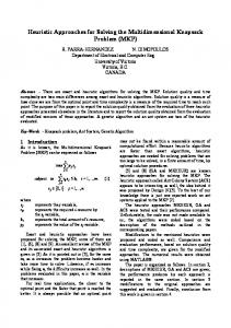
4. The gene related to the number of machines being moved in each cell or the number of machines being moved out is named Matrix [Kmc]. The alleles are limited to, …-2, -1,0,1,2…. For example, the term of K52=1 means that the number of machine 5 that are moved to cell 2 is equal to 1, and the term of K52=-1 means that the number of machine 5 that are moved out of cell 2 is equal to 1. In general, by combining the four matrices described above, the chromosome structure in each period is obtained as shown in Figures 1 or 2. It is clear that each chromosome or feasible solution consists of the H structure as shown in Figure 1 or 2, where H is the number of periods.

[[X ] | [Y ] | [K] p×r

P×r

M×C

Figure 1. Chromosome structure

10

]

| [N]M×C |

A comparison of heuristic methods for solving a cellular manufacturing model in a dynamic environment

x 11 x 12 ... x 1r y11 y12 ... y1r k 11 k 12 ... k 1C N11 N 12 ... N 1C x 21 x 22 ... x 2r y 21 y 22 ... y 2r k 21 k 22 ... k 2C N 21 N 22 ... N 2C M M M M x p1 x p2 ... x pr y p1 y p2 ... y pr k M1 k M2 ..k MC N M1 N M2 ..N MC Figure 2. Chromosome structure

(Note: The above structure will be used for SA and TS). Generation of initial population A sequential strategy is used for obtaining the initial population. In this strategy, lower bound numbers (LB) machines are first assigned to each cell randomly. Then the operations related to each part type are assigned to machines existing in cells randomly by means of ajpm values. As required, the new machines are assigned to cells or relocated between them. If possible, each operation must be assigned to the cell to which the previous operation was assigned. To transform an infeasible solution to a feasible one, a new procedure called 'Filter' is introduced. The solutions that cannot transform to feasible ones are eliminated. To avoid monotony and/or lack of variety in generations, each new solution is compared with another solution produced recently in terms of similarity. If the similarity between the new solution and another solution is less than a specific value it is accepted, otherwise it is eliminated. The similarity between two solutions (chromosomes) is defined as follows: aij − B (13) Sij = 2 × (r + C ) × Max( P, M ) where aij is the number of genes consisting of the same allele in chromosome i and chromosome j. The B variable is called the diagonal value. This variable is equal to the number of genes that always consists of zero allele in both chromosomes, due to lack of the demand for some part types or shortage of the number of operations of some part type as compared with r value (see Equation 11). This, also referred to as barren genes, is obtained from the difference between P and M. The B variable is obtained form Equation 14. ⎛ P ⎞ B = 2⎜ ∑ ei (r − OPi ) + (1 − ei )r + a(max(P, M ) − min( P, M ) )⎟ ⎝ i =1 ⎠

(14)

where : 1 ei =

if the demand for part i be nonzero ;

0

otherwise

a=

C if P>M 0 if P=M r if P [ P]ij

(17)

if [P]ij ≤ [P]ij

Stopping criterion To stop the algorithm, the following criteria are considered. 1. Number of generations: In this case, the algorithm terminates if the number of generations exceeds a specified number. 2. Time interval: In this case, the algorithm terminates if the difference between 'now' time and the time of achievement to best solution exceeds a specified time interval. GA algorithm steps The GA algorithm steps are as follows: • Initialize parameters K, G • Initialize counters r = 1 (population counter) , g = 1 (generation counter) • Do • Generate generation g as K feasible solution X1 g , X2 g ,… , Xk g • Calculate fitness of population as F(X1 g) , F(X2 g),…, F(Xk g) •

Normalize fitness of population as Z1 , Z2 , … , Zk where Z i =

•

Choose mating pool (solutions Xi that which Zi ≤ 0 )

12

F ( X ig ) − μ g

δg

A comparison of heuristic methods for solving a cellular manufacturing model in a dynamic environment

• • • • •

Do (Generate offspring for new generation) Choose one or two solutions Xi g , Xj g from current mating pool and generate offspring as follows: Choose one genetic operation randomly then: Mutation or Inversion X ig ⎯⎯ ⎯⎯⎯⎯ ⎯→ Yr

g g ⎛ F(Yr ) + F (Yr +1 ) F ( X i ) + F ( X j ) ⎞⎟ g ⎜ ≤ If F (Yr ) ≤ F ( X i ) or then ⎜ ⎟ 2 2 ⎝ ⎠ X rg +1 = Yr X rg++11 = Yr +1 or X rg +1 = X ig

(

• • • •

Re commendation or X ig , X jg ⎯Crossover ⎯ ⎯⎯→ Yr , Yr +1 or X ig ⎯⎯ ⎯⎯⎯ ⎯→ X ig

)

r = r +1 End if Loop until (r ≤ K) g=g+1 Loop until (g ≤ G )

Simulated annealing for solving he CMS model in DE The important parts of a simulated annealing algorithm for CMS are explicated in the discussion below. Solution coding The solution coding for SA is equal to GAs in Section 4.1. Initial solution An initial solution is a starting solution (point) that is to be used in the search process. In this paper, the initial solution is obtained using the approach expressed in Section 4.2. Initial temperature An initial temperature, T0, and a cooling schedule, α are used to control a series of moves in the search process. In general, the initial temperature should be high enough to allow all candidate solutions to be accepted. The cooling schedule α is the rate at which the temperature is reduced. In this research, the parameter α is obtained as follows:

α=

1 ln(1 + δ )Tr −1 1+ 3V (Tr −1 )

⇒ Tr = α Tr -1

(18)

where

1 N (Ck − C )2 ∑ N k =1 1 N C (Tr ) = ∑ C k , N k =1 V(Tr ) =

(19) (20)

Tr : Value of temperature in transition r. V(Tr) : Objective variance of accepted solutions in temperature r. C (Tr ) : Objective Mean of accepted solutions in temperature r. N : Number of accepted solutions in each temperature. δ : Rate of Cooling Number of iterations at a temperature level (N) The number of iterations at a temperature level N is equal to number of accepted solutions in each transition. The value of ‘n’ may vary from one temperature to another. It is important to spend

13

A comparison of heuristic methods for solving a cellular manufacturing model in a dynamic environment

sufficient amount of time at lower temperatures to ensure that a local optimum has been fully explored. Thus, it can be beneficial to increase the value of N either geometrically (by multiplying a factor greater than one), or arithmetically (by adding a constant factor) at each new temperature. Neighbouring solutions Neighbouring solutions are a set of feasible solutions, which can be generated from the current solution. Each feasible solution can be directly reached from current solution by a move (as a genetic operation - mutation or inversion) and this results in a neighbouring solution. Stopping criteria The number of temperature transitions is used as stopping criteria. Furthermore, the SA algorithm can be terminated when Equation 21 is satisfied.

V (Tr ) ≤ε Tr (C (T0 ) − C (Tr ) )

(21)

SA algorithm steps The SA algorithm steps are as follows: • Initialize parameters T0 , R , N , δ , ε • Initialize counters n = 0 , r = 0 • Do (Outside loop) • Set n = 0 • Generate initial solution X0 : Set XBest = Xn : Cn= F(Xn) • Do (inside loop) Mutation or Inversion • Generate Neighbouring solution Xn+1 by genetic operations : ( X n ⎯⎯ ⎯ ⎯ ⎯ ⎯⎯→ X n+1 ) • If F(Xn+1) < F(Xn) then • XBest =Xn+1 : set n = n + 1 : Cn= F(Xn) • Else • Generate random y → U(0,1) ΔCn

T

• • • • •

r if y < e then : set n = n + 1 : Cn= F(Xn) End if Loop until (n ≤ N) Calculate V(Tr) and C (Tr ) (see Equations 19 and 20) Tr+1 =α Tr ( α can be calculated by Equation 18) : set r = r + 1

•

Loop until (

V (Tr ) ≤ ε or r ≤ R) Tr (C (T0 ) − C (Tr ) )

where ε = rate of freezing and R= number of acceptable transitions.

Tabu search for solving the CMS model The notion of exploiting certain forms of flexible memory to control the search process is the central theme underlying TS. The effect of such memory may be envisioned by stipulating that TS maintains a selective history H of the number of states encountered during the search, and replaces Q(xnow) by a modified neighbourhood which may be denoted Q( H΄, xnow) ( H΄ = { m | N(m) = 0 } ; N(m) = number countered of move m). Therefore, the set H is defined as H = { m | 1 ≤ N(m) < L }. History, therefore, determines which solutions may be reached by a move from the current solution, selecting next from Q( H΄, xnow). The history or memory of tabu moves presented in the CMS model is the considered allocation of operation to cell matrix (i.e. Matrix [Y] in Figure 1). For example, if Move m = Move ( j0 ,p0 ,c0 ) ( i.e. operation j0 of part P0 is moved from current cell to cell C0 ) is chosen in which m ∉ H and generates a feasible solution xnext then N(m) =N(m) + 1 , if N(m) < L then

14

A comparison of heuristic methods for solving a cellular manufacturing model in a dynamic environment

H = H ∪ {m}. This move, therefore, can not be used while N(m) is a less than constant L. On the other hand, if N(m) = L then H = H − {m} and reinitialize N(m) = 0 then m ∈ H′ , therefore the move m can be used again. In general, the TS algorithm steps are as follows: • Initialize parameters: L , N , H = Ø (Memory is null) • Initialize counter: n = 1 • Generate initial solution X0 : XBest = X0 • Do • Choose move m • If N(m) =0 ( m ∈ H′ ) then m • Generate Neighboring solution Xn by Move m ( X n−1 ⎯⎯→ Xn) n n-1 Best n • If F(X ) < F(X ) then X =X : set n = n + 1 • Set N(m) =N(m) + 1 • Else • Set N(m) =N(m) + 1 : if N(m)=L then N(m) = 0 • End if • Loop until (n ≤ N) • Print XBest where N= Number of accepted solutions as a stopping criterion.

Computational results To compare the heuristic solutions 10 test problems solved by GA, SA, TS and Lingo were examined. The results obtained are shown in Table 1 and 2. Some problems (with 'high dimensions') could not be solved within a reasonable time by Lingo on a PC as illustrated in Table 1, because of the presence of large number of variables and constraints. The best solution value of the objective function and computational time for each approach is indicated in Table 1. Except for problem 2 (highlighted by asterisk), the remainder stopped at a global optimum. The CMS constant parameters in all the test problems were as follows: • B (batch size) = 50. • γ (cost of inter cell move) = 40. • The number of feasible machines for each operation = 2. GA parameters • The number of populations in each generation (K) = 100, 150, 200. • The maximum number of generation (G) (stopping criteria) = 100. • The variance of generation (stopping criteria) = 0.01. SA parameters • The number of solutions accepted in each temperature (N) = 100. • The rate of cooling (δ) = 0.01. • The rate of freezing (ε) =0.01. • The number of temperature transitions (stopping criteria) = 100. TS parameters The number of tabu countered for each move (L) = M ; M= the number of machines. The number of solutions accepted (N) (stopping criteria) = 100. To solve the problem use of a Pentium Ш,1.1 Gz computer was made. The optimal solution was obtained by using Lingo 6 software. The heuristic algorithm was developed by the application of Visual Basic 6. Tables 1 and 2 illustrate the computational results. By considering the proposed CM model, the presented algorithms are able to find and report the near-optimal and promising solutions

15

A comparison of heuristic methods for solving a cellular manufacturing model in a dynamic environment

within reasonable time. This indicates the success of the proposed algorithms. In general, the obtained results can be divided into the following parts: 1. All approaches almost always found the near-optimal solution utilizing lower computational time than the optimal algorithm. 2. On average, the SA algorithm finds better solutions compared to GAs and TS within reasonable computational time. Table 1. Comparisons of solutions obtained by heuristics and Lingo 6 Test Problem Part × Machine, Cell, Period

Lingo 6

Genetic Algorithms

Simulated Annealing

Tabu Search

Objective

Time

Objective

Time

Objective

Time

Objective

Time

5×5 , C=2 , H=2

9361

00:01:55

10768

00:00:03

10449

00:00:30

10691

00:01:15

6×6 , C=3 , H=3

13730 *

03:29:06

13268

00:00:46

12807

00:02:00

13733

00:30:00

7×6 , C=3 , H=3

16218

00:01:35

19692

00:00:58

19115

00:04:40

20259

00:05:00

8×6 , C=3 , H=2

18245

00:02:41

19371

00:07:48

19371

00:13:12

19793

00:04:00

8×7 , C=3 , H=3

17148

04:41:30

20478

00:12:50

20228

00:13:15

19442

00:40:10

9×8 , C=3 , H=2

18164

02:47:18

18680

00:54:30

18890

00:09:30

18915

00:00:54

10×10 , C=3 , H=2

15880

00:23:57

16593

00:04:00

16851

00:00:09

17915

00:20:30

12×10 , C=3 , H=2

N/A

N/A

27755

00:09:06

27713

00:08:00

28628

00:05:00

20×15 , C=4 , H=3

N/A

N/A

95874

00:34:18

87800

00:10:30

95414

00:04:20

30×20 , C=4, H=2

N/A

N/A

73085

01:27:30

71984

00:21:00

74313

00:40:00

* - Local solution Table 2. Objective differences between heuristic solutions and the best solution Test Problem

Var & Cons

GAs

SA

TS

Part × Machine, Cell, Period 5×5 , C=2 , H=2

401 , 152

13%

10%

12%

6×6 , C=3 , H=3

972 , 260

Better of Lingo

Better of Lingo

0%

7×6 , C=3 , H=3

1444 , 272

17%

15%

19%

8×6 , C=3 , H=2

1360 , 277

5%

5%

7%

8×7 , C=3 , H=3

1507 , 414

16%

15%

11%

9×8 , C=3 , H=2

1826 , 288

2%

3%

3%

10×10 , C=3 , H=2

1452 , 338

4%

5%

11%

12×10 , C=3 , H=2

1656 , 395

0.1%

Best

3%

20×15 , C=4 , H=3

8500 , 1438

0.001%

Best

0.03%

30×20 , C=4, H=2

8588 , 1064

1%

Best

3%

Conclusion In this paper, a mathematical model based on nonlinear mixed-integer programming is presented for designing cellular manufacturing systems (CMSs) in dynamic states. Three meta heuristics are proposed and designed to solve the above model. The proposed simulated annealing (SA) algorithm finds and reports near-optimal solutions in a shorter average time interval compared to genetic algorithms (GAs) and tabu search (TS) in most of the test problems. The solutions obtained by the GA program are receiving increasing credit and justification in real-world situations. Experimentally, if the number of machines, parts, cells, and period is greater than 10, 10, 3, and 2 respectively, the Lingo software running on a PC was unable to extract any solution for the proposed mathematical model in dynamic states. In general, the chance of achieving an optimal solution is increased by improving the

16

A comparison of heuristic methods for solving a cellular manufacturing model in a dynamic environment

GA principle presented by the six factors because this operation can be used to generate neighbouring solutions in either SA or TS.

References Bagley, J. D. (1976) The behavior of adaptive systems which employ genetic and correlation algorithms Doctoral Dissertation, University of Michigan. Benjaafar, S. & Sheikhzadeh, M. (2000) Design of flexible plant layouts IIE Transactions 32(4) pp.309-322. Boctor, F. F. (1991) A linear formulation of the machine-part cell formation problem International Journal of Production Research 29(2) pp.343-356. Cavicchio, D. J. (1972) Adaptive search using simulated evolution Doctoral Dissertation, University of Michigan. Chen, M. (1998) A mathematical programming model for systems reconfiguration in a dynamic cellular manufacturing environment Annals of Operations Research 77(1) pp.109-128. Gen, M. & Cheng, R. (1997) Genetic algorithms and engineering design (New York: John Wiley & Sons). Glover, F. & Laguna, M. (1997) Tabu search (Boston: Kluwer Academic Publishers). Goldberg, D. E. (1989) Genetic algorithm in search optimization, and machine learning (Reading, MA: Addison-Wesley). Gupta, Y., Gupta, M., Kumar, A. & Sundram, C. (1995) Minimizing total inter-cell and intera-cell moves in cellular manufacturing: a genetic algorithm International Journal of Computer Integrated Manufacturing 8(2) pp.92-101. Graves, R. (1996) Rensselear’s electronics agile manufacturing research institute: a research and development collaborative th enterprise in electronics Proceeding of the 5 Industrial Engineering Research Conference Minneapolis MN pp.602-605. Harahalakis, G., Nagi, R. & Proth, J. (1990) An efficient heuristic in manufacturing cell formation to group technology applications International Journal of Production Research 28(1) pp.185-198. Holland, J. H. (1975) Adaptation in natural and artificial systems (Ann Arbor: University of Michigan Press). Joines, J., Culberth, C. & King, R. (1996) Manufacturing cell design: an integer programming model employing genetic algorithms IIE Transactions 28(1) pp.69-85. Kirkpatrick, F., Gelatt, C. & Vecci, M. (1983) Optimization by simulated annealing Science Magazine 220(4598) pp.671-680. Logendran, R., Ramakrishna, P. & Srikandarajah, C. (1994) Tabu search based heuristic for cellular manufacturing systems in the presence of alternative process plans International Journal of Production Research 32(2) pp.273-297. Metropolis, N., Rosenbluth, A., Rosenbluth, M., Teller, A. & Teller, E. (1953) Equation of state calculations by fast computing machines Journal of Chemical Physics 21(6) pp.1087-1092. Mungwatanna, A. (2000) Design of cellular manufacturing systems for dynamic and uncertain production requirement with presence of routing flexibility Blacksburg State University Virginia. Montreuil, B. & Laforge, A. (1992) Dynamic layout design given a scenario tree of probable futures European Journal of Operational Research 63(2) pp.271-286. Rosenberg, R.S. (1967) Simulation of genetic population with biochemical properties Doctoral Dissertation, University of Michigan. Seifoddini, H. (1990) A probabilistic model for machine cell formation Journal of Manufacturing Systems 9(1) pp.69-75. Sofianopoulou, S. (1997) Application of simulated annealing to a linear model for the formulation of machine cells in group technology International Journal of Production Research 35(2) pp.501-511. Song, S. & Hitomi, K. (1996) Integrating the production planning and cellular, layout for flexible cellular manufacturing Production Planning and Control 7(6) pp.585-593. Vakharia, A. & Chang, Y. (1997) Cell formation in group technology: a combinatorial search approach International Journal of Production Research 35(7) pp.84-97. Venugopal, V. & Narendran, T. (1992) A genetic algorithm approach to the machine component grouping problem with multiple objectives Computer and Industrial Engineering 22(4) pp.469-480. Wilhelm, W., Chiou, C. & Chang, D. (1998) Integrating design and planning considerations in cellular manufacturing Annals of Operations Research 77(1) pp.97-107. Yang, T. & Peters, B. (1998) Flexible machine layout design for dynamic and uncertain production environments European Journal of Operational Research 108(1) pp.49-64.

17