A Comparison of Topology Control Algorithms for Ad-hoc Networks Gaurav Srivastava, Paul Boustead, Joe F.Chicharo School of Electrical, Computer and Telecommunication Engineering, University of Wollongong, NSW, Australia. Email:
[email protected],
[email protected], Joe
[email protected] Abstract— Topology control in mobile ad-hoc networks allows better spatial reuse of the wireless channel and control over network resources. Topology control algorithms tend to optimise network power usage by keeping the topology connected. In this paper, we provide an overview of a range of centralised and distributed topology control algorithms proposed in literature. We also provide a comparison of these algorithms and suggest which algorithms may perform best. We comment on the partitioning, routing, scheduling and latency issues that may arise due to topology adaptations in a mobile ad-hoc network. Keywords—Mobile ad-hoc networks, Topology control algorithms, Issues, Comparison
I. I NTRODUCTION A mobile ad hoc network (MANET) is a group of mobile wireless nodes working together to form a network. Such networks can exist without a fixed infrastructure and can work in an autonomous manner. Every mobile device has a maximum transmission power which determines the maximum transmission range of the device. As nodes are mobile, the link connection between two devices can break depending on the spatial orientation of the nodes. Two mobile wireless devices out of communication range, can use other devices within their communication range to relay packets. As ad-hoc networks may not require any fixed infrastructure, it makes them very flexible to deploy in different scenarios. MANETs have numerous applications such as sensor networks, disaster relief, military operations, business and home applications. Some of the network constraints in MANETs are limited bandwidth, low battery power of nodes, frequent link unreliability due to mobility. The topology of a multi-hop wireless network is a “set of communication links between node pairs used explicitly or implicitly by routing mechanisms” [1]. A topology can depend on uncontrollable factors such as node mobility, weather, interference, noise as well as controllable factors such as transmission power, directional antennas [2] and multi-channel communications [1]. Inappropriate topology can reduce the impact of network capacity by limiting spatial reuse of the communication channel and decrease network robustness. For example, if the topology is too sparse then the network can get partitioned. However, topology control can provide better control over network resources such as battery power and reduce redundancy in network communications. Centralised topology control algorithms rely on global topology information to make topology adaptation decisions. Distributed topology control algorithms rely on partial link state information such as neighbour count to maintain network connectivity. Section II of this paper describes the working of the cen-
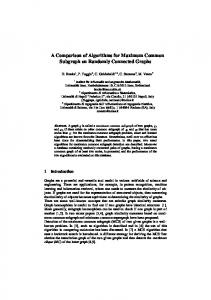
tralised and distributed topology control algorithms. Section III discusses the computational and scalability issues and provides a comparison of algorithms. Section IV outlines the related issues in applying the topology control algorithms in mobile ad-hoc networks. Section V concludes the paper. II. E XISTING T OPOLOGY C ONTROL A LGORITHMS Since the advent of DARPA packet radio networks in the early 1970s, numerous topology control algorithms have been proposed for ad-hoc networks. Such topology control algorithms deal with limitations of wireless networks, such as power consumption and network capacity optimisation. As shown in Figure 1, the topology control algorithms may be categorised as (a) centralised and (b) distributed in nature. Lines in the figure represent the direct descendants. The distributed algorithms are further categorised into two parts (a) Connectivity Aware, which try to optimise network connectivity and (b) Capacity aware, which try to achieve higher capacity by reducing the contention in the network. The following section describes the algorithms and categorise them according to their characteristics. Current Topology Control Algorithms Centralised
Distributed
RNG MST
Connectivity Aware
Capacity Aware
Connect
LILT
MobileGrid
NTC
LINT
COMPOW
minR
Dist−RNG Dist−NTC
Biconn−Augmnet
Fig. 1. Categorisation of Topology Control Algorithms
A. Centralised Topology Control Algorithms In centralised topology control algorithms a particular network node is responsible for evaluating an optimum network topology based on the locations of the other network nodes. The location information along with the transmission range of the individual nodes is used to form a link between a node pair. The algorithms differ mainly in the techniques used in evaluating the optimum topology. This section describes a number of different centralised topology control algorithms and makes a characteristic comparison between them which is illustrated in Table I.
The performance metric represents the worst case scenario for each algorithm. A.1 Relative Neighbourhood Graph (RNG) The relative neighbourhood graph of N node network, RNG(N) are exactly those pairs (Ni , Nj ) of points for which there is no node Nz such that kli − lz k < kli − lj k and klj − lz k < kli − lj k where lx denotes the position vector of node x [3]. Hence the edge between Ni and Nj is only valid if there is no other node between Ni and Nj . There are various algorithms for two-dimensional and threedimensional space for creating RNG. The computational cost of the brute-force algorithm is O(N 3 ) [4]. Supowit [5] designed the first cone based search, sequential time algorithm for computing RNG with the computation cost in the order of O(N logN ). A.2 Minimum Spanning Tree (MST) The MST of a graph defines the smallest subset of edges that keeps the graph in one connected component [6]. MST is a sub graph of RNG. There are two main algorithms, Kruskal’s [7] and Prim’s [7] algorithm for computing MST. Kruskal’s algorithm chooses edges of the graph with minimum weight. As the edges (E) are arranged in an increasing order, the procedure takes O(logE) steps. The computation cost of the algorithm is O(ElogE). Prim’s algorithm builds the MST by putting an arbitrary node into the tree. This eliminates the search step required in the Kruskal’s algorithm. The edges are added to the graph if they are smaller than the previous edges already in the graph. The computation cost of the algorithm is O(E + N logN ). A.3 Connect Connect algorithm [1] is similar to MST. It works by iteratively merging node pairs until the entire network is connected. Connect initialises ‘N’ clusters, one for each node. Node pairs are selected in an increasing order of their mutual distance. The transmission power of each node is increased until they are able to reach each other. Once the nodes are connected the corresponding clusters are unified. The process is repeated until the entire network is connected. A power increase may add more than one edge to the induced graph. Such additional edges other than the selected node pairs are called ‘side-effect’ edges [1]. A ‘side-effect’ edge may form a loop with other edges. A postprocessing phase is used to remove the side-effect edges and make the power assignment minimal. The total cost of the algorithm is O(N 2 logN ) [1]. A.4 Noble Topology Control Algorithm (NTC) NTC algorithm proposed by Hu [8] modifies a Delaunay Triangulation (DT) graph to achieve the desired network capacity and network connectivity. The algorithm starts with a DT graph, which provides a reliable backbone topology [8]. The edges are sorted in the order of decreasing length. All edges longer than length R are removed from the graph. The sorting operation is the bottle-neck of the algorithm because the number of possible edges E is O(E 2 ) and hence the cost is in the order of O(E 2 logE) [8].
A.5 Minimum Radius Graph (minR) This algorithm assumes that nodes have common transmission power. The algorithm searches for the smallest power to keep the network connected. The connectivity of the network is checked after every step increase in power. The search operation for checking the network connectivity incurs a cost of O(N 2 ) [9]. The total cost of the algorithm is estimated to be O(N 2 P ), where P is the number of power increments. The algorithm assumes that all network devices operate on a common power level, which is an unrealistic assumption. Choosing a common power level also increases the power redundancy in the network as it may introduce side-effect edges in the connected components. A.6 Biconn-Augment Biconn-Augment [1] adapts the connected network to a biconnected network. Biconnectivity ensures that there is always at least two links connecting a node to every other node, hence the topology will remain connected even after a node goes down. In order to achieve biconnectivity the algorithm first tries to identify the biconnected components using Depth First Search (DFS) [1]. The nodes are then selected in increasing order of their mutual distance and joined only if they are in different biconnected components. This process is repeated until the network is biconnected. A post processing phase similar to Connect ensures per-node power minimisation. The algorithm has a computation cost of O(N 2 logN ) [1]. B. Connectivity Aware Distributed Topology Control Algorithms Connectivity aware topology control algorithms try to adjust the neighbour count to maintain connectivity and stability in the network. Each node maintains ‘neighbour’ information. A node becomes a ‘neighbour’ if it is within the transmission range of the other nodes. Such neighbour information is periodically updated when a node moves out/in the communication range of each other. For example, AODV routing protocol uses “Hello” messages to exchange link-state information [10]. A bidirectional link is established when both nodes are within each others transmission range. The remainder of this section describes the working of some of the existing connectivity aware topology control algorithms and heuristics. A characteristic comparison of the connectivity aware algorithms is shown in Table II. B.1 Local Information No Topology (LINT) LINT proposed by Ramanathan et al. [1] uses locally available neighbour information collected by routing protocols to keep the degree of neighbours bound. All network nodes are configured with three parameters, the desired node degree d d , a high threshold of the node degree dh and a low threshold of node degree dl . A node periodically checks the number of its active neighbours. If the degree is greater than dd , the node reduces its operational power. If the degree is less than dd the node increases its operational power. If neither is true then no action is taken. The increase/decrease in transmission power is bounded by maximum/minimum power settings of the radio. The min-
imum overhead of checking the neighbour count of an N node network is in the order of O(N ) as every node needs to check its neighbour count at least once. B.2 Local Information Link-State Topology (LILT) LILT is another algorithm/heuristic presented by Ramanathan et al. [1] which exploits the global topology information for recognising and repairing network partitions. There are two main parts of LILT, Neighbour Reduction Protocol (NRP) and Neighbour Addition Protocol (NAP). NRP reduces the transmission power to maintain the node degree around a certain configured value where as NAP increases the transmission power to establish additional links. The overhead of checking the neighbour count of a N node network is in the order of O(N ) When executing NRP and NAP a node receiving a routing update determines whether it is connected or biconnected. If a node does not receive any updates then it may be in a disconnected state. If the topology is biconnected then no action is taken. If the topology is disconnected then the node increases its transmission power to the maximum possible value. If the topology is connected and not biconnected, the node tries to achieve bi-connectivity. Bi-connectivity is reached by evaluating the closest ‘articulation point’ (AP). An AP is a node whose removal will partition the network. The overhead of evaluating the AP using DFS is in the order of O(N + E). The overall overhead is in the order of O(2N + E), which is obtained by summing the neighbour adaption and AP evaluation overheads.
active node rejects the request from any other node except the nearest active node. The process is repeated until the number of adjacent edges are equal to the fixed value or no more nodes (in range) are available for matching. Non-active nodes do not join the distributed matching procedure. An active node changes into a non-active one if it has enough links or cannot find an active node within its maximum transmission range. The overall communication complexity of the algorithm for a N node network is O(N L) [8]. C. Capacity Aware Distributed Topology Control Algorithms Capacity aware topology control take into acount that the network nodes cause interference which impacts the communication of other nodes in the vicinity. It was shown by Gupta and Kumar [11] that √ the per node capacity may be estimated in the order of O(1/ N ), with N being the number of nodes in the network. The transmission of surrounding nodes effect the signal to noise ratio (SNR) of other network communications. The SNR of an ongoing communiation decreases with the number of neighbouring communications and is proportional to the interference power of these communications. The capacity aware approach tries to alter the network topology by reducing the communication interference due to other nodes. This section outlines two capacity aware distributed topology control algorithms proposed in the literature. A characteristic comparison is summarised in Table II. C.1 MobileGrid
B.3 Distributed Relative Neighbourhood Graph (Dist-RNG) Dist-RNG proposed by Borbash et al.[4] is a distributed algorithm for computing a RNG based topology. When executing Dist-RNG a node Ni grows its transmission power until the nearest neighbour Nj is found in the uncovered region. Once a node is found, an edge (Ni , Nj ) is added to RNG. If there are more than one node then a corresponding edge for each of them is added to the RNG. By using the new found neighbour Nj an angle θj is calculated. This angle θj defines a cone that spans the area covered by Nj . θ donates the set of angles which define cones that jointly span the covered regions. Initially θ is set to zero. θj is merged with θ and the whole process is repeated until the entire region (2π) around Ni is spanned or the maximum power is reached. The computational overhead of the algorithm is in the order of O(N logN ) for a N node network [4].
MobileGrid proposed by Liu et al. [12] is a distributed topology control algorithm which, maintains a specific contention index (CI). CI is a product of node density 1 (ρ) and area size (A). In order to maintain global CI, all nodes try to keep the local CI bound to a specific value. The local estimate of contention index at the ith node is evaluated from the number of one hop neighbours(Ni). Each node looks up a particular optimisation table to determine whether it is operating around an optimal value of CI. The optimal values of CI are evaluated beforehand through simulations and hard-coded in the network nodes. A node adjusts it transmission range to keep the CI value bound. MobileGrid uses CI values between [3,9] to maximise the network capacity [12]. This approach is similar to LINT and hence checking CI is performed at least once which incurs a minimum overhead in the order of O(N ).
B.4 Distributed Novel Topology Control Algorithm (DistNTC)
C.2 Common Power level (COMPOW)
In Dist-NTC all nodes broadcast their own existence and collect neighbour information within their maximum transmission range R [8]. Furthermore, every node finds adjacent DT neighbours within R. Each node keeps only a fixed number of shortest edges and informs other ends about abandoned edges and rejects any edge abandoned by a neighbour. Network nodes which have less than specified edges are classified as ‘active’. Every active node joins a ‘distributed matching procedure’ and finds the nearest active neighbour and sends a request packet to it and waits for a reply [8]. Network links, that may arise due to the distributed matching procedure are called non-basic links (L) [8]. If the reply is acknowledged by the receiver then an edge is added. Each
Network nodes executing COMPOW [13] operate on the smallest power level to reach maximum network connectivity. COMPOW maintains a routing table at different power levels. Each routing table exchanges link state updates at different powers to generate the route information. The optimum power of a node is the smallest power level whose routing table has the same number of entries as that of a routing table at the maximum power level [13]. COMPOW reduces the transmission power redundancy and interference by selecting the maximum operational power settings to reach the furthest neighbour node. In the worst case scenario the algorithm will incur a cost of O(P N ), 1 The
number of nodes per unit area.
TABLE I C HARACTERISTICS OF THE
Algorithms RNG MST Connect NTC
CENTRALISED TOPOLOGY CONTROL ALGORITHMS .
CO Strategy O(N logN ) Cone based search O(E + N logN ) Tree formation
Advantages Low power topology Low power topology
O(N 2 logN ) O(E 2 logE)
Disadvantages Low FT and high APs Low FT and high APs and high overheads Low FT and high overheads High overheads
Iterative cluster migration Low power topology DT graph formation and High FT sorting edges minR O(N 2 P ) Search for minimum power High FT due to high Same transmission power to maintain overall network power redundancy for all nodes, high overheads connectivity and low APs Biconn − Augment O(N 2 logN ) Iterative cluster migration High FT and low APs High overheads and DFS due to biconnectivity CO=Computation overheads. FT=Fault tolerance. AP=Articulation points. E=Total number of edges. N=Total number of nodes in the network. P=Number of power increments. TABLE II C HARACTERISTICS OF THE DISTRIBUTED TOPOLOGY CONTROL ALGORITHMS .
Algorithms Strategy
Tables
CO
Checking APs O(N ) NO O(2N + E) YES
Maintaining a specific node degree 1 Maintaining a specific node degree and checking 1 for APs Dist − NTC Maintaining a specific node degree and computing 1 O(N L) NO local DT graphs Dist − RNG Maintaining local RNGs 1 O(N logN ) NO MobileGrid Maintain CI 1 O(N ) NO COMPOW Evaluating an optimum power level P O(P N ) NO P=Power levels. CO=Computation overhead. FT=Fault tolerant. AP=Articulation point. L=Number of non-basic links. E=Total number of edges. N=Total number of nodes in the network. LINT LILT
where P are the number of power levels and N are the number of network nodes. III. D ISCUSSION Centralised topology control algorithms require one network node to compute and disseminate the topology information in the network. All link-sate information needs to be relayed back to the central node, which computes the optimum topology. This procedure introduces extra processing and communication overheads on the coordinating node as well as its neighbours, which participate in broadcasting the new topology information into the network. In a MANET, the network nodes are mobile, thus the centralised algorithms may take longer to converge to an optimum topology. From the central topology control algorithms discussed, RNG has the least computational overheads which makes RNG more scalable as compared to the rest of the algorithms. However, Biconn-Augment has high computational cost, but the algorithms ensures biconnectivity in the network. Biconnectivity in the network assists in reducing APs and improves the fault tolerance (FT) as there may be more than one node supporting a particular link. Distributed topology control algorithms limit the topology
control decisions to a selected part of the network. All topology control decisions are made on the local link-sate information of a node and its neighbouring nodes. The distributed nature of the algorithm reduces the bottle neck of a centralised controller and the overheads of disseminating the link-state information to the coordinating node. Maintaining a specific node degree may work well in a uniform node distribution, but in the case of non-uniform distribution, the network can become partitioned and the node degree approach can cause unreliability in the network. LINT, DistRNG, MobileGrid do not address the network partitioning issue that may arise due to transmission range alterations, specially in heterogeneous topology distributions. LILT addresses the partitioning issue by checking for APs and maintaining connectivity with them. Dist-NTC uses active nodes to maintain connectivity. An active node overcomes a disconnected state by maintaining a fixed number of closest edges. The choice of edges like ‘node degree’ in LINT may depend on many parameters such as network density and network size. The bottleneck of Dist-NTC is the search operation to evaluate DT neighbours. MobileGrid uses CI, which is similar to the node degree approach of LINT. Increasing power levels of a radio may also lead to side-effect edges which may cause higher node degree and undesired con-
tention 1 [11]. This situation becomes worse in a dense network where most of the nodes are distributed close to each other. A change of few meters of transmission range can lead to large number of neighbours. The NAP and NRP can work against each other, when the desired node degree or topology state is not met. In this scenario LINT, LILT, Dist-NTC and MobileGrid will take longer time to converge to a desired node degree. All distributed topology control algorithms need to maintain a local view of the topology and the link state information. This information can be stored in a table format which can be periodically updated with the changing link state of the network. However the overheads in case of COMPOW are larger compared to the rest of the the algorithms, as it maintains topology information at different power levels. Disseminating topology information at different power levels can consume a significant amount of bandwidth. Network nodes have to exchange link state information at every power setting. This information can be expensive specially if the number of power levels are high. For example, the Nth power level will automatically contain information about the N − 1th power level. The process also creates redundancy in the amount of information maintained at each node and introduce large memory and communication overheads. From the distributed topology control algorithms discussed, LILT incorporates the neighbour adaption approach of LINT, MobileGrid and Dist-NTC. LILT is also more adaptive to different topology distributions as it tries to maintain connectivity with the APs and keep the network in a biconnected state, thereby improving the network’s falut tolerance. The overheads of the algorithms are comparable to other distributed approaches which provides an advantage over other algorithms.
perceives changes in the link state information of the network. Scheduling topology control decisions in distributed approaches is complicated as topology adaptation need to be coordinated to avoid/minimise disruptions in existing communications [1]. Inappropriate topology adaptations can result in unnecessary delay in communication. None of the topology control algorithms take node mobility into account while making topology adaptation decisions. Due to node mobility, the topology adaptation can reduce network connectivity specially if the network nodes are moving away form each other. Including node mobility information and movement pattern during topology adaptation can make the topology control scheme more adaptive and stable in a mobile environment. V. C ONCLUSION In this paper we have classified the different centralised and distributed topology control algorithms proposed for ad-hoc networks. It is evident that topology control in ad-hoc network can conserve power usage by exploiting the spatial orientation of network nodes. However, it is crucial to address issues such as topology control overheads, latency, scheduling and mobility when designing the topology control algorithms/protocols. R EFERENCES [1] [2] [3]
IV. R ELATED I SSUES Topology control in a network can alter the link-state of network nodes and therefore routing protocols have to refresh the route information every time a topology control algorithm is executed. Routing protocols rely on the link-sate information of the network to compute the various routing paths. In a worst case scenario the routes have to be rebroadcasted after every topology adaptation. This procedure is expensive as route requests and setup consumes significant overheads. Link state updates due to topology control, along with the link update due to movement of nodes may consume substantial amount of bandwidth. In practice, power adaptation can also introduce latency in the network as wireless devices can take some time in switching to a different power level. The amount of latency depends on the radio frequency (RF) components of the device and firmware implementation. However, altering of power levels can be in the order of seconds, which may have significant impact on the end-to-end delay of network applications. Due to latency, it is essential to coordinate the topology adaptation algorithms at an appropriate time. The latency issue introduces another concern of scheduling of the topology control algorithms. Scheduling topology control in a large network is a challenging issue. The centralised approach requires one network node to periodically broadcast the optimum topology or when it 1 Contention is the communication delay that the nodes experience in the presence of other nodes in the area.
[4]
[5] [6] [7] [8] [9]
[10] [11] [12]
[13]
Ramanathan R. and Rosales-Hain R., “Topology control of multihop wireless networks using transmit power adjustment,” in Proc. IEEE INFOCOM, 2000. Zhuochuan Huang, Chien-Chung Shen, Srisathapornphat, and Jaikaeo C., “Topology control for ad hoc networks with directional antennas,” in Computer Communications and Networks, 2002. Jerzy W. Jaromczyk and Godfried T. Toussaint, “The relative neighbourhood graphs and their relatives,” in Proceedings of the IEEE, Vol. 80, No 9, Sept. 1992. Chi-Fu Huang, Yu-Chee Tseng, Shih-Lin Wu, and Jang-Ping Sheu, “Distributed topology control algorithm for multihop wireless networks ,” in Neural Networks, 2002. IJCNN ’02. Proceedings of the 2002 International Joint Conference on , Vol.1, Pages: 355-360, 2002. Kenneth J. Supowit, “The relative neighbourhood graph with application to minimum spannig trees,” in Journal of the ACM,vol. 30, no. 3, pp 428448, 1983. Ning Li, Jennifer C. Hou, and Lui Sha, “Design and Analysis of an MSTBased Topology Control Algorithm,” in INFOCOM 2003. Nicos Christofides, Graph Theory : An Algorithmic Approach, Academic press, 1975. Hu L, “Topology control for multihop packet radio networks,” in Communications, IEEE Transactions on , Vol.41, Iss.10, Pages: 1474- 1481, 1993. Esther Jennings and Clayton Okino, “Topology control for efficient information dissemination in ad-hoc networks,” in International Symposium on Performance Evaluation of Computer and Telecommunication Systems SPECTS 2002, 2002. Perkins C.E and Bending-Royer E.M., “Ad hoc On-Demand Distance Vector Routing Protocol for Mobile Ad Hoc Networks,” in draft-ietfmanet-aodv-11.txt,, June 2002. Gupta P. and Kumar P.R, “The capacity of Wireless Networks,” in Transactions and information theory, Mar. 2000. Jilei Liu and Baochun Li, “Mobilegrid: capacity-aware topology control in mobile ad hoc networks,” in Computer Communications and Networks, 2002. Proceedings. Eleventh International Conference on, Vol., Pages: 570- 574, 2002. Narayanaswamy S., Kawadia V., Sreenivas R.S., and Kumar P.R., “Power Control in Ad-Hoc Networks: Theory, Architecture, Algorithm and Implementation of the COMPOW Protocol.,” in Proceedings of the European Wireless Conference, Next Generation Wireless Networks: Technologies, Protocols, Services and Applications, Feb. 2002.