A Comparison of Algorithms for Maximum Common Subgraph on Randomly Connected Graphs H. Bunke1, P. Foggia2, C. Guidobaldi1,2, C. Sansone2, M. Vento3 1 Institut für Informatik und angwandte Mathematik, Universität Bern, Neubrückstrasse 10, CH-3012 Bern, Switzerland
[email protected] 2 Dipartimento di Informatica e Sistemistica, Università di Napoli “Federico II”, via Claudio, 21 I-80125 Napoli, Italy {foggiapa, cguidoba, carlosan}@unina.it 3 Dipartimento di Ingegneria dell’Informazione ed Ingegneria Elettrica, Università di Salerno, via P.te Don Melillo, 1 I-84084 Fisciano (SA), Italy
[email protected]
Abstract. A graph g is called a maximum common subgraph of two graphs, g1 and g2, if there exists no other common subgraph of g1 and g2 that has more nodes than g. For the maximum common subgraph problem, exact and inexact algorithms are known from the literature. Nevertheless, until now no effort has been done for characterizing their performance. In this paper, two exact algorithms for maximum common subgraph detection are described. Moreover a database containing randomly connected pairs of graphs, having a maximum common graph of at least two nodes, is presented, and the performance of the two algorithms is evaluated on this database.
1
Introduction
Graphs are a powerful and versatile tool useful in various subfields of science and engineering. There are applications, for example, in pattern recognition, machine learning and information retrieval, where one needs to measure the similarity of objects. If graphs are used for the representation of structured objects, then measuring the similarity of objects becomes equivalent to determining the similarity of graphs. There are some well-known concepts that are suitable graph similarity measures. Graph isomorphism is useful to find out if two graphs have identical structure [1]. More generally, subgraph isomorphism can be used to check if one graph is part of another [1,2]. In two recent papers [3,4], graph similarity measures based on maximum common subgraph and minimum common supergraph have been proposed. Detection of the maximum common subgraph (MCS) of two given graphs is a wellknown problem. In [5], such an algorithm is described and in [6] the use of this algorithm in comparing molecules has been discussed. In [7] a MCS algorithm that uses a backtrack search is introduced. A different strategy for deriving the MCS first obtains the association graph of the two given graphs and then detects the maximum clique (MC) of the latter graph [8,9].
Both, MCS and MC detection, are NP-complete problems [10]. Therefore many approximate algorithms have been developed. A survey of such algorithms, including an analysis of their complexity, and potential applications is provided in [11]. Although a significant number of MCS detection algorithms have been proposed in the literature, until now no effort has been spent for characterizing their performance. Consequently, it is not clear how the behaviour of these algorithms varies as the type and the size of the graphs to be matched changes from an application to another. The lack of a sufficiently large common database of graphs makes the task of comparing the performance of different MCS algorithms difficult, and often an algorithm is chosen just on the basis of a few data elements. In this paper we present two exact algorithms that follows different principles. The first algorithm searches for the MCS by finding all common subgraphs of the two given graphs and choosing the largest [7]; the second algorithm builds the association graph between the two given graphs and then searches for the MC of the latter graph [12]. Moreover we present a synthetically generated database containing pairs of randomly connected pairs of graphs, in which each pair has a known MCS. The remainder of the paper is organized as follows. In Section 2 basic terminology is introduced and the first algorithm to be compared is described. The second algorithm to be compared is described in Section 3. In Section 4 the database used is presented, while experimental results are reported in Section 5. Finally future work is discussed and conclusions are drawn in Section 6.
2
A space state search algorithm for detecting the MCS
The two following definitions will be used in the rest of the paper: Definition 2.1: A graph is a 4-tuple g = ( V, E, a, ß ), where − V is the finite set of vertices (also called nodes) − E ⊆ V × V is the set of edges − a : V → L is a function assigning labels to the vertices − ß : E → L is a function assigning labels to the edges Edge (u,v) originates at node u and terminates at node v. Definition 2.2: Let g1 = ( V1, E1, a1, ß1 ) and g2 = ( V2, E2, a2, ß2 ) be graphs. A common subgraph of g1 and g2, cs(g1 ,g2), is a graph g = ( V, E, a, ß ) such that there exist subgraph isomorphisms from g to g1 and from g to g2. We call g a maximum common subgraph of g1 and g2, mcs(g1,g2), if there exists no other common subgraph of g1 and g2 that has more nodes than g. Notice that, according to Definition 2, mcs(g1,g2), is not necessarily unique for two given graphs. We will call the set of all MCS of a pair of graphs their MCS set. According to the above definition of MCS, it is also possible to have graphs with isolated nodes in the MCS set. This is in contrast with the definition given in [7], where a MCS of two given graphs is defined as the common subgraph which contains the maximum number of edges (we could call it edge induced MCS, in contrast with the method described in this paper, which is node induced). Then the case of a MCS containing unconnected nodes is not considered in [7]. Consequently, the algorithm proposed in this section, although derived from the one described in [7] by McGregor,
is more general. It can be suitably described through a State Space Representation [13]. Each state s represent a common subgraph of the two graphs under construction. procedure MCS(s,n1,n2) begin if (NextPair(n1,n2)) then begin if (IsFeasiblePair(n1,n2)) then AddPair(n1,n2); CloneState(s,s'); while(s' is not a leaf of the search tree) begin MCS(s',n1,n2); BackTrack(s'); end Delete(s'); end end procedure
Fig. 1: Sketch of the space state search for maximum common subgraph detection. This common subgraph is part of the MCS to be eventually formed. In each state a pair of nodes not yet analyzed, the first belonging to the first graph and the second belonging to the second graph, is selected (whenever it exists) through the function NextPair(n1,n2). The selected pair of nodes is analyzed through the function IsFeasiblePair(n1,n2)that checks whether it is possible to extend the common subgraph represented by the actual state by means of the this pair. If the extension is possible, then the function AddPair(n1,n2)actually extends the current partial solution by the pair (n1,n2). After that, if the current state s is not a leaf of the search tree, it copies itself through the function CloneState(s,s’), and the analysis of this new state is immediately started. After the new state has been analyzed, a backtrack function is invoked, to restore the common subgraph of the previous state and to choose a different new state. Using this search strategy, whenever a branch is chosen, it will be followed as deeply as possible in the search tree until a leaf is reached. It is noteworthy that every branch of the search tree has to be followed, because - except for trivial examples - is not possible to foresee if a better solution exists in a branch that has not yet been explored. It is also noteworthy that, whenever a state is not useful anymore, it is removed from the memory through the function Delete(s). The first state is the empty-state, in which two null-nodes are analyzed. A pseudo-code description of the MCS detection algorithm is shown in Fig 1. Let N1 and N2 be the number of nodes of the first and the second graph, respectively, and let N1 ≤N2. In the worst case, i.e. when the two graphs are completely connected with the same label on each node and the same label on each edge, the number of states s examined by the algorithm is: 1 1 (1) S = N 2 !⋅ ( N − N ) ! + K + ( N − 1) ! 1 2 2 For the case N1 = N2 = N and N >>1, eq.(1) can be approximated as follows:
S ≅ e ⋅N! Notice that only O(N1) space is needed by the algorithm.
3
( 2)
An MCS algorithm based on clique detection
The Durand-Pasari algorithm is based on the well known reduction of the search of the MCS between two graph to the problem of finding a MC in a graph [12]. The first step of the algorithm is the construction of the association graph, whose vertices corresponds to pair of vertices of the two starting graphs having the same label. The edges of the association graph represent the compatibility of the pair of vertices to be included; hence, MCS can be obtained by finding the MC in the association graph. The algorithm for MC detection generates a list of vertices that represents a clique of the association graph using a depth-first search strategy on a search tree, by systematically selecting one vertex at a time from successive levels, until it is not possible to add further vertices to the list. A sketch of the algorithm is in Fig. 2. procedure MCS_DP(vert_list) begin level = length(vert_list); null_count = count_null_vertices(vert_list); clique_length = level – null_count; if (null_count >= best_null_count_so_far) then return; else if (level == max_level) then save(vert_list); best_null_count_so_far = null_count; else P = set of vertices (n1,n2) having n1==level; foreach(v in P ∪ { NULL_VERTEX }) begin if (is_legal(v, vert_list)) then MCS_DP(vert_list + v); end if end end if end procedure
Fig. 2: Sketch of the maximum clique detection algorithm. When a vertex is being considered, the forward search part of the algorithm first checks to see if this vertex is a legal vertex, and if it is the algorithm next checks to see if the size of the new clique formed is as large or larger than the current largest clique, in which case it is saved. A vertex is legal if it is connected to every other vertex already in the clique. At each level l, the choice of the vertices to consider is limited to the ones which correspond to pairs (n1, n2) having n1=l. In this way the algorithm ensures that the search space is actually a tree, i.e. it will never consider twice the same list of vertices. After considering all the vertices for level l, a special vertex, called the null vertex, is added to the list. This vertex is always considered legal, and can be added more than once to the list. This special vertex is used to carry
the information that no mapping is associated to a particular vertex of the first graph being matched. When all possible vertices (including the null vertex) have been considered, the algorithm backtracks and tries to expand along a different branch of the search tree. The length of the longest list (excluding any null vertex entries) as well as its composition is maintained. This information is updated, as needed. If N1 and N2 are the number of vertices of the starting graphs, with N1≤N2 , the algorithm execution will require a maximum of N1 levels. Since at each level the space requirement is constant, the total space requirement of the algorithm is O(N1). To this, however, the space needed to represent the association graph must be added. In the worst case the association graph can be a complete graph of N1⋅N2 nodes. In the worst case the algorithm will have to explore (N2+1) vertices at level 1, N2 at level 2, up to (N2− N1+2) at level N1. Multiplying these numbers we obtain a worst case number of states ( N 2 + 1)! S= ( N 2 + 1)( N 2 ) K ( N 2 − N 1 + 2) = (3) ( N 2 − N1 + 1)! which, for N1=N2 reduces to O(N⋅N!).
4
The Database
During the last years the pattern recognition community recognized the importance of benchmarking activities for validating and comparing the results of proposed methods. Within the Technical Committee 15 of the International Association for Pattern Recognition (IAPR-TC15) the characterization of the performance achieved by graph matching algorithms revealed to be particularly important due to the growing need of using matching algorithms dealing with large graphs. To this concern, two artificially generated databases have been presented at the last IAPR-TC15 workshop [14, 15]. The first one [14] describes the format and the four different categories contained in a database of 72,800 pairs of graphs, developed for graph and subgraph isomorphism benchmarking purposes. The graphs composing the whole database have been distributed on a CD during the 3rd IAPR-TC15 and are also publicly available on the web at the URL: http://amalfi.dis.unina.it/graph. A different way for building a graph database has been proposed in [15]. Here the graphs are obtained starting from images synthetically generated by means of a set of attributed plex grammars. Different classes of graphs are therefore obtained by considering different plex grammars. The databases cited above are not immediately usable for the purpose of benchmarking algorithms for MCS. In fact, the first database can be used with graph (or subgraph) isomorphism algorithms and provides graphs with no labels. Also the second database has not been developed for generating graphs to be used in the context of MCS algorithms. To overcome these problems we decided to generate another database of synthetic graphs with random values for the attributes, since any other choice requires making assumptions about the application dependent model of the graphs to be generated. In particular, we assumed, without any loss of generality, that attributes are represented by integer numbers with a uniform distribution over a certain interval. In fact, the purpose of the attributes in our benchmarking activity is simply to restrict the possible node or edge pairings; hence there is no need to have structured attributes. The most important parameter characterizing the difficulty of the matching
problem is the number M of different attribute values: obviously the higher this number, the easier is the matching problem. Therefore, it should be important to have different values of M in a database. In order to avoid the need to have several copies of the database with different values of M, we chose to generate each attribute as a 16bit value, using a random number generation. In this way, a benchmarking activity can be made with any M of the form 2k , for k not greater than 16, just by using, in the attribute comparison function, only the first k bits of the attribute. As regards the kind of graphs, we chose to include in the database randomly connected graphs, i.e. graphs in which it is assumed that the probability of an edge connecting two nodes is independent on the nodes themselves. The same model as proposed in [1] has been adopted for generating these graphs: it fixes the value η of the probability that an edge is present between two distinct nodes n and n′ . The probability distribution is assumed to be uniform. According to the meaning of η, if N is the total number of nodes of the graph, the number of its edges will be equal to ηN·(N-1). However, if this number is not sufficient to obtain a connected graph, further edges are suitably added until the graph being generated becomes connected. η 0.05
0.1
0.2
# of nodes (N) 20 25 30 10 15 20 25 30 10 15 20 25 30
# of nodes of the MCS 2, 6, 10, 14, 18 2, 7, 12, 17, 22 3, 9, 15, 21, 27 3, 5, 7, 9 4, 7, 10, 13 2, 6, 10, 14, 18 2, 7, 12, 17, 22 3, 9, 15, 21, 27 3, 5, 7, 9 5, 7, 10, 13 2, 6, 10, 14, 18 2, 7, 12, 17, 22 3, 9, 15, 21, 27
# of pairs 500 500 500 400 400 500 500 500 400 400 500 500 500
Table 1. The database of randomly connected graphs for benchmarking algorithms for MCS.
The generated database is structured in pairs of graphs having a MCS of at least two nodes. In particular, three different values of the edge density η have been considered: 0.05, 0.1 and 0.2. For each value of η, graphs of different size N, ranging from 10 to 30 have been taken into account. Values of N equal to 10 and 15 have not been considered for η=0.05, since in these cases it was not possible to have connected graphs without adding a significant number of extra edges. Five different percentages of the values of N have been considered for determining the size of the MCS, namely 10%, 30%, 50%, 70% and 90%. This choice allows us to verify the behavior of the algorithms as the ratio between the size of the MCS and the value of N varies. Then, for each value of N and for each chosen percentage, 100 pairs of graph have been generated, giving rise to a total of 6100 pairs. Note that for
values of N equal to 10 and 15, the 10% value was not considered as it would determine a MCS size less than two nodes. Table 1 summarizes the characteristic of the graphs composing the database. The MCS size refers to the case in which M=216.
5
Experimental Results
In order to make an unbiased comparison of the two algorithms presented in Sections 2 and 3, we have developed an implementation of both in C++, using the VFLib class library available at http://amalfi.dis.unina.it/graph. The code has been compiled using the gcc 2.96 compiler, with all optimizations enabled. The machines used for the experiments are based on the Intel Celeron processor (750MHz), with 128 MB of memory; the operating system is a recent Linux distribution with the 2.4.2 kernel version. A set of Python scripts have been used to run the two algorithms on the entire database and to collect the resulting matching times. As we have explained in the previous section, the database contains 16 bits attributes, that can be easily employed to test the algorithms with different values of the parameter M. Since both algorithms have a time complexity that grows exponentially with the number of nodes, it would be impractical to attempt the matching with a too low value of M. We have chosen to employ values of M proportional to the number of nodes in the graphs being matched, in order to keep the running times within a reasonable limit. In particular, we have tested each graph pair in the database with three M values equal to 33%, 50% and 75% of the number of nodes. The resulting matching times are shown in Fig 3. Notice that one of the database parameters, the number of nodes of the generated MCS, does not appear in the figure. In fact, in order to reduce the number of curves to be displayed, we have averaged the times over the different MCS sizes. It should be also considered that, for different values of M, the actual size of the MCS may vary. In fact if M is large, some node pairs are excluded from the MCS because of their attribute values; if M is small, the same pairs may become feasible for inclusion. Hence, by not reporting separately the times for different MCS sizes it becomes easier to compare the results corresponding to different values of M. Examining the times reported in the figure, it can be noted that while both algorithms exhibit a very rapidly increasing time with respect to the number of nodes, they show a behavior quite different from each other with respect to the other two considered parameters that is, M and the graph density η. As regards M, it can be seen that the matching time decreases when M gets larger. But while for low values of M the Durand-Pasari algorithm performs usually better than the McGregor one, for high values of M the situation is inverted. This can be explained by the fact that the Durand-Pasari algorithm is based on the construction of an association graph, which helps reducing the computation needed by the search algorithm when the search space is large (small M) because the compatibility tests are, in a sense, “cached” in the structure of the association graph; on the other hand, the association graph construction imposes a time (and space) overhead, that is not repaid when the search space is small (large M). For the graph density, we notice that the dependency of the matching time on η is opposite for the two algorithms. In fact, while the time for Durand-Pasari decreases for larger values of η, the time for McGregor increases.
An explanation of this difference is that, for Durand-Pasari, an increase in the graph density enables the algorithm to prune more node pairs on the basis of the node connections. In the McGregor algorithm, instead, this effect is compensated by the increase of the number of edge compatibility tests that must be performed at each state, to which the Durand-Pasari is immune because of the use of the association graph. Randomly Connected Graphs - M =33% 10000 Durand-Pasari
McGregor
η=0.2
1000
η=0.1 η=0.05
a)
Times [sec]
100 10
η=0.1 1
η=0.05
0.1
η=0.2
0.01 0.001 10
15
20
25
N
30
Randomly Connected Graphs - M =50% 1000 Durand-Pasari
McGregor
η=0.2
100
b)
Times [sec]
10
η=0.05 η=0.1 η=0.1
1 0.1
η=0.2 η=0.05
0.01 0.001 0.0001 10
15
20
25
N
30
Randomly Connected Graphs - M =75% 10 Durand-Pasari
McGregor
η=0.2
1
c)
Times [sec]
η=0.05 0.1
η=0.1 η=0.1
0.01
η=0.2
η=0.05 0.001
0.0001 10
15
20
25
30 N
Fig. 3: Results obtained for M=33% a),50% b),75% c) of N, as a function of N and η.
6
Conclusions and Perspectives
In this paper, two exact algorithms for MCS detection have been described. Moreover a database containing randomly connected pairs of graphs having a MCS of at least two nodes has been presented, and the performance of the two algorithms has been
evaluated on this database. Preliminary comparative tests show that for graphs with a low density it is more convenient to search for the MCS by finding all the common subgraphs of the two given graphs and choosing the largest, while for high edge density, it is efficient to build the association graph of the two given graphs and then to search for the MC of the latter graph. At present the database presented in the paper contains 6100 pairs of randomly connected graphs. A further step will be the expansion of the database through the inclusion of pairs of graphs with more of nodes. Besides, the inclusion of other categories graphs, such as regular meshes (2-dimensional, 3-dimensional, 4-dimensional), irregular meshes, bounded valence graphs, and irregular bounded graphs will be considered. Moreover further algorithms for MCS will be implemented and their performances characterized on this database. A more precise measure of the performance could be obtained with a further parameter in the database, namely the size s of the MCS in each pair of graphs.
References [1] [2]
[3] [4] [5] [6]
[7] [8] [9] [10] [11] [12] [13] [14]
[15]
J.R. Ullmann, “An Algorithm for Subgraph Isomorphism”, Journal of the Association for Computing Machinery, vol. 23, pp. 31-42, 1976. L.P. Cordella, P. Foggia C. Sansone, M. Vento, “An Improved Algorithm for Matching Large Graphs”, Proc. of the 3rd IAPR-TC-15 International Workshop on Graph-based Representations, Italy, pp. 149-159, 2001. H. Bunke X. Jiang and A. Kandel, “On the Minimum Supergraph of Two Graphs”, Computing 65, Nos. 13 - 25, pp. 13-25, 2000. H. Bunke and K.Sharer, “A Graph Distance Metric Based on the Maximal Common Subgraph”, Pattern Recognition Letters, Vol. 19, Nos. 3-4, pp. 255-259, 1998. G. Levi, “A Note on the Derivation of Maximal Common Subgraphs of Two Directed or Undirected Graphs”, Calcolo, Vol. 9, pp. 341-354, 1972. M. M. Cone, Rengachari Venkataraghven, and F. W. McLafferty, “Molecular Structure Comparison Program for the Identification of Maximal Common Substructures”, Journal of Am. Chem. Soc., 99(23), pp. 7668-7671 1977. J.J. McGregor, “Backtrack Search Algorithms and the Maximal Common Subgraph Problem”, Software Practice and Experience, Vol. 12, pp. 23-34, 1982. C. Bron and J. Kerbosch, “Finding All the Cliques in an Undirected Graph”, Communication of the Association for Computing Machinery 16, pp. 575-577,1973. B. T. Messmer, “Efficient Graph Matching Algorithms for Preprocessed Model Graphs”, Ph.D. Thesis, Inst. of Comp. Science and Appl. Mathematics, University of Bern, 1996. M. R. Garey, D. S. Johnson, “Computers and Intractability: A Guide to the Theory of NPCompleteness”, Freeman & Co, New York, 1979. I. M. Bomze, M. Budinich, P. M. Pardalos, and M. Pelillo, “The Maximum Clique Problem”, Handbook of Combinatorial Optimization, vol. 4, Kluwer Academy Pub., 1999. P. J. Durand, R. Pasari, J. W. Baker, and Chun-che Tsai, “An Efficient Algorithm for Similarity Analysis of Molecules ”, Internet Journal of Chemistry, vol. 2, 1999. N. J. Nilsson, “Principles of Artificial Intelligence”, Springer-Verlag, 1982. P. Foggia, C. Sansone, M.Vento, “A Database of Graphs for Isomorphism and Sub-Graph Isomorphism Benchmarking”, Proc. of the 3rd IAPR TC-15 International Workshop on Graph-based Representations, Italy, pp. 176-187, 2001. H. Bunke, M. Gori, M. Hagenbuchner C. Irniger, A.C. Tsoi, “Generation of Images Databases using Attributed Plex Grammars”, Proc. of the 3rd IAPR TC-15 International Workshop on Graph-based Representations, Italy, pp. 200-209, 2001.