Surveillance Program [California Air Resources Board,. 2000]. Rc of natural gas ..... remote sensingâbased automobile combustion ratios as. 0.033 ± 0.004 and ...
Click Here
JOURNAL OF GEOPHYSICAL RESEARCH, VOL. 115, D11303, doi:10.1029/2009JD012236, 2010
for
Full Article
A comparison of tracer methods for quantifying CO2 sources in an urban region Sonja Djuricin,1 Diane E. Pataki,1,2 and Xiaomei Xu2 Received 10 April 2009; revised 16 October 2009; accepted 7 January 2010; published 4 June 2010.
[1] The relative contribution of anthropogenic (natural gas and gasoline combustion) and biogenic (aboveground and belowground respiration) CO2 sources has previously been quantified with the 13C, 18O, and 14C isotopes of CO2. The unique combination of isotopic signatures of each source allows for top‐down attribution of sources using atmospheric measurements. Other tracers of CO2 include carbon monoxide (CO), which is a direct tracer of fossil fuel combustion‐derived CO2 as CO and CO2 are evolved at specific ratios (RCO/CO2) during combustion depending on fuel source and combustion efficiency. We used the 13C, 18O, and 14C tracers to partition between natural gas, gasoline, and aboveground and belowground respiration during four sampling events in the Los Angeles basin. Additionally, we compared the effectiveness of the independent CO tracer with the 14 C tracer to distinguish between anthropogenic and biogenic CO2. The three isotope tracer results showed that during the sampling period, fossil fuel combustion was not a dominant source of CO2 and aboveground respiration contributed up to approximately 70% of CO2 sources during the spring. However, the percent fossil fuel CO2 calculated by the CO tracer was not entirely consistent with the fossil fuel CO2 calculated by 14C, which predicted up to ∼70% of winter CO2 from fossil fuel sources. The CO tracer was useful for showing diurnal patterns of CO2 sources. However, combustion RCO/CO2 values vary significantly, which poses a challenge for accurately identifying CO2 sources. Detailed local information about RCO/CO2 is required to effectively utilize the CO tracer for quantifying sources of CO2. Citation: Djuricin, S., D. E. Pataki, and X. Xu (2010), A comparison of tracer methods for quantifying CO2 sources in an urban region, J. Geophys. Res., 115, D11303, doi:10.1029/2009JD012236.
1. Introduction [2] Monitoring atmospheric CO2 sources is increasingly of interest for implementing greenhouse gas regulations and policy. However, even in heavily urbanized areas, the atmosphere contains both biologically derived CO2 as well as CO2 from fossil fuel combustion. The relative contribution of anthropogenic and biogenic sources of CO2 in urban regions has been found to vary on relatively short diurnal and seasonal scales [Pataki et al., 2006] and also across urban to rural gradients of land use [Pataki et al., 2007]. In these studies, the stable isotopes 13C and 18O of CO2 were used to distinguish between CO2 sources with unique isotope signatures [Pataki et al., 2003a, 2003b, 2006; Zimnoch et al., 2004; Zondervan and Meijer, 1996]. However, there are uncertainties and limitations to using stable isotopes to trace CO2 sources. While 13C is particularly useful for identifying natural gas combustion, which is more depleted 1 Department of Ecology and Evolutionary Biology, University of California, Irvine, California, USA. 2 Department of Earth System Science, University of California, Irvine, California, USA.
Copyright 2010 by the American Geophysical Union. 0148‐0227/10/2009JD012236
in 13C than gasoline (petroleum), another tracer is needed to distinguish between gasoline and respiration, which have similar carbon isotopes ratios (d 13C). The oxygen isotope ratio (d18O) can generally be used to distinguish between biogenic and anthropogenic CO2 because evaporative enrichment of H18 2 O in plants and soils imparts a unique signature to evolved CO2 in respiration. Application of this tracer, therefore, requires detailed modeling of evaporative enrichment and CO2 equilibration with plant and soil water pools. Because plant and soil water generally differs significantly in isotopic composition, a priori knowledge of the proportional contributions of aboveground versus belowground respiration may also be required [Pataki et al., 2003b, 2007]. [3] Radiocarbon (14C) is another isotopic tracer that is useful for distinguishing between anthropogenic and biogenic sources of CO2 [Kuc et al., 2003; Levin et al., 2003, 2008; Levin and Karstens, 2007; Levin and Rodenbeck, 2008; Takahashi et al., 2002; Turnbull et al., 2006]. Fossil fuel combustion releases CO2 with no 14C because the half‐life of 14C (5730 years) is much shorter than the age of fossil fuels. In contrast, modern background and biogenic CO2 is enriched in 14C from cosmogenic radiation sources and residual sources from aboveground nuclear weapons
D11303
1 of 13
D11303
DJURICIN ET AL.: CO2 SOURCE TRACER COMPARISON
testing the 1950s and 1960s. This provides a very large range of end‐members for tracing even relatively small amounts of fossil fuel‐derived CO2. However, sample preparation and analysis is generally more time‐consuming and costly than stable isotope analysis, which limits sample collection and analysis. In contrast, carbon monoxide (CO) is a product of combustion that can be measured continuously. Because the local excess biogenic sources of CO are negligible in the urban environment, previous studies have used the independent CO tracer to resolve the contribution of fossil fuel‐derived CO2 to the atmosphere [Gamnitzer et al., 2006; Potosnak et al., 1999; Turnbull et al., 2006]. Combustion yields CO in addition to CO2 at specific ratios depending on the source and the combustion efficiency. Therefore, the CO/CO2 ratio may provide continuous information about CO2 sources in order to monitor diurnal and seasonal patterns of energy use and respiratory fluxes. While CO/CO2 measurements are relatively inexpensive and have the advantage of providing continuous data, a disadvantage is in the uncertainty in the combustion ratio of various fossil fuel sources. [4] The purpose of this study is twofold: first, we wished to combine the stable isotope tracers 13C and 18O with 14C in order to better resolve the biogenic contribution of CO2 to the urban atmosphere, and to be able to distinguish between aboveground and belowground respiration rather than making a priori assumptions about their relative contributions. This would greatly reduce the uncertainty associated with using isotopes to trace urban CO2 sources. Second, we wished to compare the effectiveness of CO/CO2 ratios with the isotope tracers. Our analysis using three isotopes (13C, 18 O and 14C) allowed us to partition locally derived CO2 into four sources: natural gas combustion, gasoline combustion, belowground respiration, and aboveground respiration using a mass balance approach. The use of CO/CO2 ratios allowed us to investigate diurnal differences in fossil fuel‐derived CO2 inputs into the atmosphere. Finally, the CO and isotope tracer‐based partitioning methods were compared directly with simultaneous CO, CO2 and 14C measurements. We propose that three 13C, 18O and 14C tracers used together will allow us to partition between four biogenic and anthropogenic CO2 sources, and that the accuracy of these results will depend on how well the local source end‐members are known. We also predict that the CO tracer will not be as effective as 14C in quantifying the relative abundance of fossil CO2 in the urban atmosphere due to the uncertainty in the combustion efficiency of anthropogenic CO2 sources.
2. Methods 2.1. Study Site [5] All air samples were collected from the University of California, Irvine. The study site was located 6 km from the coast within the Los Angeles basin, approximately 58 km south of the city of Los Angeles. The region is highly urbanized, with a total population in the Los Angeles‐ Riverside‐Orange County consolidated metropolitan statistical area of 16 million reported by the U.S. census in 2000. This semiarid ecosystem is characterized by prevailing onshore breezes and a Mediterranean climate with approximately 172 mm of precipitation annually and an average air
D11303
temperature of 17.1°C. Offshore atmospheric transport (“Santa Ana winds”) occurs most frequently in fall and winter. During these events, air masses move from inland to the coastal region instead of the prevailing pattern of transport of marine air inland. 2.2. CO2 and CO Mixing Ratios [6] Continuous CO2 and CO mixing ratios were recorded between October 2007 and February 2008. Air was sampled from an inlet located approximately 6.7 m from the ground and passed from a 2.5mm filter to the gas analyzers. CO mixing ratio was measured with a 48i TLE CO Analyzer (Thermo Fisher Scientific Inc., Waltham, MA, United States), along with a continuous filter wheel purge by a low flow of N2. The CO analyzer was calibrated with zero CO air and a 9.26 mmol · mol−1 EPA traceable standard several times during the sampling period. CO2 mixing ratio was measured with an infrared gas analyzer (LI‐820, LI‐COR Inc., Lincoln, NE, United States) after passing through a Magnesium perchlorate trap. The analyzer was calibrated hourly with zero CO2 air and two WMO traceable ‘low’ and ‘high’ standards. The ‘low’ standard gases used over the course of the sampling period had CO2 mixing ratios of 395–411 mmol mol−1 (depending on the tank used) while the ‘high’ standard tanks varied between 599 and 606 mmol mol−1. These concentrations were selected as they represented the upper and lower bounds of the CO2 concentrations that we expected to measure in the atmosphere. Five minute averages of CO and CO2 mixing ratios were recorded with a CR10x data logger (Campbell Scientific Inc., Logan, UT, United States). The precision of these measurements was 0.01 mmol mol−1 for CO and 0.2 mmol mol−1 for CO2. 2.3. Flask Sampling [7] Air samples used for stable isotope and radiocarbon analyses were collected in evacuated To‐Can 24174 and 22107 model 6 L canisters (Restek, Bellefonte, PA, United States). Prior to collection, canisters were heated while connected to a vacuum in order to remove water vapor. Flask samples were collected from a height of 6.7 m on 22– 23 October 2007; 11–13 December 2007; 10 February 2008; and 11 April 2008. Collected air was passed through a 1.0 mm air filter and a magnesium perchlorate desiccating trap before being routed to the canisters. We attempted to collect flask samples during nighttime to exclude the effect of photosynthesis on the isotopic composition of the atmosphere [Flanagan and Ehleringer, 1998], and in particular during early morning periods of maximum atmospheric stability to capture locally derived CO2. [8] CO2 for isotope analysis was isolated from air samples with a cryogenic CO2 extraction vacuum line as described by Xu et al. [2007a]. The stable isotopes 18O and 13C were analyzed with a Dual Inlet Isotope Ratio Mass Spectrometer (Delta‐Plus, Thermo, Waltham, MA, United States), and N2O corrections of +0.23‰ and +0.30‰ were made for d13C and d18O measurements of CO2, respectively [Sirignano et al., 2004]. Radiocarbon analysis was performed using the Accelerator Mass Spectrometer (AMS) at the W.M Keck AMS Lab at UC Irvine, following target preparation as outlined by Xu et al. [2007a]. The analytical errors for d 13C and d 18O were 0.1 and 0.2‰, respectively,
2 of 13
D11303
DJURICIN ET AL.: CO2 SOURCE TRACER COMPARISON
D11303
and belowground respiration; c refers to the CO2 mixing ratio of a component; and d13C, d18O and D14C are 13C, 18O and 14C isotope signatures of source end‐members and D14C (‰) d 13C (‰) d 18O (‰) measured CO2. We neglected to include a term for coal‐ −8.6 ± 0.03b 41.5 ± 0.09b derived CO2 as there are no coal‐fired plants in the surBackground 54.0 ± 0.2a rounding area. Anthropogenic [12] CO2 and CO mixing ratios and stable isotope ratios of Natural gas −1000 −39.8c – −44.0d 23.5 ± 0.3e background air were estimated with data from the NOAA Gasoline −954.0 ± 4.0f −25.5f – −28.3g 23.5 ± 0.3e Earth System Research Laboratory (NOAA‐ESRL, http:// Biogenic www.esrl.noaa.gov/gmd/dv/ftpdata.html) Trinidad Head, −26.2 ± 0.2g 34.0 – 62.2i Aboveground respiration 166 ± 100h California, and POCN30 (Pacific Ocean site off the coast of h g i Belowground respiration 166 ± 100 −26.2 ± 0.2 20.1 – 22.3 California at 30° latitude) sites data sets. For D14C, we used a 14 Point Barrow, AK [Xu et al., 2007b]. measurements at Point Barrow, AK C reported by Xu et al. b THD, POC30 stations; NOAA‐ESRL. [2007b]. c Microturbine combustion samples, UCI. d [13] The 14C end‐members of natural gas and gasoline Blasing et al. [2004]. e typically contain no radiocarbon due to their age. However, Kroopnick and Craig [1972]. f Vehicle exhaust samples; Irvine, California. recent additions of ethanol derived from ‘modern’ sources g Pataki et al. [2003b]. of corn into gasoline may result in slightly small amounts of h Turnbull et al. [2006]. 14 i C. Exhaust samples from eight vehicles chosen randomly Modeled plant and soil respiration [Flanagan et al., 1997]. in a parking lot were analyzed for 13C and 14C end‐members of gasoline and diesel fuel combustion (Table 1). Because no differences were found in d13C of gasoline versus diesel 14 and 2–3‰ for D C based on measurements of duplicates fuel, similar to Bush et al. [2007], the values were comand secondary standards. bined. Samples were collected after passing air through a [9] Stable isotope data are reported in conventional d magnesium perchlorate trap as described by Bush et al. notation, [2007], and d13C and D14C were measured with continu� � ¼ Rsample =Rstandard � 1 � 1000; ð1Þ ous flow IRMS and AMS, respectively. Natural gas was assumed to be completely depleted in radiocarbon. The 13C where R is the ratio of the heavy to the light isotope. end‐member for natural gas was reported as −40.2 ± 0.5‰ Values were referenced to the V‐PDB standard for d13C by Newman et al. [2008] and −44.0‰ by Blasing13et al. [2004]. We also made direct measurements of d C of and the V‐SMOW standard for d 18O. local natural gas by sampling exhaust from a Capstone C60 [10] For radiocarbon, values were expressed in D notation Microturbine Generator on the university campus. The � � was −39.8‰. �14 C ¼ Fe�ðy�1950Þ=8267 � 1 � 1000; ð2Þ measured value from this sample collection For biogenic respiration, we applied a D14C value of 166 ± 100‰ from Turnbull et al. [2006] and a d13C value of where y is the current year. F is the fraction modern or, the −26.2‰ from Pataki et al. [2003a, 2003b]. The end‐member 14 12 C/ C ratio of the sample with respect to 14C/12C of the for biogenic respiration is particularly uncertain for D14C and Oxalic Acid I standard and has been corrected for mass‐ likely to be different for autotrophic versus heterotrophic dependent fractionation [Stuiver and Polach, 1977]. respiration; hence, we placed a large uncertainty estimate on this value for both aboveground and belowground respira2.4. Three Isotope Tracer Based CO2 Source tion. We did not have sufficient information to specify difPartitioning ferent values for aboveground versus belowground [11] In order to partition measured CO2 into source respiratory CO2 sources, so we used the same value with components, we applied mass balance, large uncertainty rather than making a priori assumptions ct ¼ cb þ cn þ cg þ cp þ cs ; ð3Þ about the isotopic disequilibrium between18CO2 entering and leaving ecosystems. Instead, we used d O to distinguish between aboveground and belowground CO2, as the end‐ �13 Ct ct ¼ �13 Cb cb þ �13 Cn cn þ �13 Cg cg þ �13 Cp cp þ �13 Cs cs ; members can be determined with process models. [14] Natural gas and gasoline end‐members for d 18O were ð4Þ assumed to be 23.5 ± 0.3‰, the isotopic signature of atmospheric oxygen [Kroopnick and Craig, 1972], although we note the possibility of deviations from this theoretical �18 Ot ct ¼ �18 Ob cb þ �18 On cn þ �18 Og cg þ �18 Op cp þ �18 18Os cs ; et al., 2008]. The soil and plant respið5Þ value [Schumacher ration 18O signal was modeled according to Flanagan et al. [1997] and Pataki et al. [2003b] using local water, atmo18 �14 Ct ct ¼ �14 Cb cb þ �14 Cn cn þ �14 Cg cg þ �14 Cp cp þ �14 Cs cs ; spheric and meteorological data. We used d O measure18 O = −8.4‰) and groundwater ments of local irrigation (d ð6Þ (d18O = −6.8‰) as source water d18O in our evaporative where the subscripts t, b, n, g, p and s represent total, enrichment models as local vegetation relies primarily on background, natural gas, gasoline, aboveground respiration, these two water sources rather than precipitation, which is infrequent in this semiarid ecosystem. We applied these
Table 1. Isotopic End‐Members of Urban CO2 Sources Used in Mass Balance Equations (3)–(6)
3 of 13
D11303
D11303
DJURICIN ET AL.: CO2 SOURCE TRACER COMPARISON Table 2. Reported and Measured Natural Gas and Gasoline Combustion RCO/CO2 Ratios Source
RCO/CO2
Gasoline [REVEAL, 1999] Fossil fuel (Environmental Protection Agency, online report, 2004) Gasolinea [California Air Resources Board, 2000]; see auxiliary material Figure S2 Natural gas (UC Irvine Central Plant; see auxiliary material Figure S1) Gasolineb [California Air Resources Board, 2000]
0.019 ± 0.0029 0.02 ± 0.005 0.028 ± 0.00058 0.034 ± 0.037 0.042 ± 0.0013
a The gasoline ratio from the Vehicle Surveillance Program, calculated by removing outliers 3 standard deviations away from the mean value. b The mean value of the Vehicle Surveillance Program data.
source water d18O values in plant and soil enrichment models [Flanagan et al., 1997] as source water for soil evaporation and stem water d 18O for plants, as plants are known to not fractionate against 18O during water uptake [Ehleringer and Dawson, 1992]. Other variables used in the enrichment models included temperature and humidity recorded by a weather station on top of our campus building, and water vapor d 18O collected from the same height as flask samples were collected (d18O = −13.9‰). Finally, we assumed steady state leaf water conditions during late afternoon and evening periods due to the lack of information needed to quantify nonsteady state evaporative enrichment [Cernusak et al., 2002]. [15] Equations (3)–(6) were solved with the inverse modeling approach described by Xu et al. [2006] and Pataki et al. [2007]. This approach uses a Bayesian probabilistic inversion technique [Xu et al., 2006; Leonard and Hsu, 1999; Tarantola, 2005] to derive a set of solutions and their associated uncertainties given a plausible set of prior constraints. The analysis derives a posterior probability density function (PDF) of solutions to equations (3)–(6) with an a priori PDF based on the known ranges of possible end‐members (Table 1).The prior constraint for each of the cn, cg, cp and cs variables was a range defined as ct‐cb. Constants in the simulation were d13Cb, d18Ob, d18On, d18Og, D14Cb, D14Cg and D14Cn as described in Table 1. For the other end‐members: d13Cn, d13Cg, d 13Cp, d 13Cs, d18Op, d 18Os, D14Cp, and D14Cs, we designated upper and lower bounds for these estimates based on literature and error values (Table 1). The simulations were run 20,000 times. 2.5. CO‐Based Partitioning [16] Continuous CO and CO2 data from 22 October 2007 to 10 February 2008 were used for source partitioning using CO/CO2 ratios. Data from individual days were separated into weekday and weekend periods and further divided into averages for the following time intervals: 0000–0230, 0730– 1000, 1200–1600, and 1730–2000 local time (LT). Background mixing ratios of CO and CO2 obtained from NOAA‐ESLR were subtracted from total mixing ratios in order to obtain ‘excess’ mixing ratios. Daily time interval averages of excess CO were plotted against those of excess CO2, and a slope was calculated using linear regression.
Finally, these slopes were used to calculate the fraction of fossil fuel present in the air using the simple mixing model, Rm ¼ Rc f f þ Ro ð1 � f f Þ;
ð7Þ
where R is the ratio of CO/CO2 and ff is the fraction of fossil fuel. The subscripts m, c and o refer to measured, combustion and other CO/CO2 ratios, respectively. Ro was set to zero for biological sources. [17] Rc values (Table 2) were obtained from the literature, e.g., Rc = 0.02 ± 0.005 (Environmental Protection Agency, Trends in greenhouse gas emissions and sinks: 1990–2002, in EPA Summary Report GHG Emissions Inventory 2004, http://www.epa.gov/climatechange/emissions/downloads06/ 04ES.pdf), as well as estimated from local data. Vehicle Rc was estimated from CO and CO2 emissions data obtained from the California Air Resources Board (CARB) Vehicle Surveillance Program [California Air Resources Board, 2000]. Rc of natural gas was estimated using emissions data from on‐campus power generation facility that utilizes natural gas at the University of California, Irvine. [18] In order to directly compare the partitioning results from the CO tracer with 14C, we also differentiated between fossil and nonfossil CO2 using D14C. �14 Cs ¼ �14 Cf f f þ �14 Cr ð1 � f f Þ;
ð8Þ
where D14C is the radiocarbon signature of the source air (s) mixing with background air, fossil fuel CO2 (f) and biological respiration 14C signatures (r). We used the Keeling plot linear regression mixing model [Keeling, 1958, 1961] to determine the isotopic signature of the source (D14Cs), � �14 Ct ¼ cb �14 Cb � �14 Cs ð1=ct Þ þ �14 Cs ;
ð9Þ
where the subscripts t, b and s represent the total, background and source air, respectively. Alternatively, when the background CO2 mixing ratio and 14C signature are known, a simple mass balance model,
4 of 13
ct ¼ cb þ cf þ cr
ð10Þ
�14 Ct ct ¼ �14 Cb cb þ �14 Cf cf þ �14 Cr cr ;
ð11Þ
D11303
DJURICIN ET AL.: CO2 SOURCE TRACER COMPARISON
D11303
Figure 1. Daily minimum and maximum mixing ratios between 22 October 2007 and 10 February 2008. The daily minimum and maximum mixing ratios are shown for (a) CO2 and (b) CO. can also be applied. We compared both of these approaches to CO‐based partitioning.
3. Results 3.1. CO and CO2 Mixing Ratio [19] CO and CO2 data collected from 22 October 2007 and 10 February 2008 represent a continuous data set with
the exception of a time period from 1–15 January 2008. Daily minimum CO2 mixing ratios varied between 380 and 400 mmol mol−1 while maximum mixing ratios varied over a larger interval, up to approximately 600 mmol mol−1 (Figure 1). Daily CO mixing ratios also varied approximately between 0.2 mmol mol−1 and 3.5 mmol mol−1. Average CO2 diurnal mixing ratios were highest during early morning hours, reaching approximately 440 mmol
5 of 13
D11303
DJURICIN ET AL.: CO2 SOURCE TRACER COMPARISON
D11303
Figure 2. Average diurnal mixing ratios for (a) CO2 and (b) CO. Averages were calculated with the data set spanning between 22 October 2007 and 10 February 2008. Shaded areas represent the standard deviation of individual points. mol−1 (Figure 2). The diurnal pattern of CO for the same period shows peaks of approximately 0.6 mmol mol−1 during early mornings and evenings. 3.2. Flask Sample CO2 Isotopes and Partitioning [20] The d13C, d18O and D14C values for air samples collected on 22–23 October 2008, 11–13 December 2008, 1 February 2008 and 11 April 2008 are shown in Figure 3. The isotope values for the October samples varied between −9.3 and −7.5‰ for d13C, 40.2 and 44.2‰ for d18O, and 12.0 to 46.0 for D14C. These samples were collected during Santa Ana wind conditions, in the initial days of the extensive 2007 southern California wildfires. The d13C, d18O and D14C values for the December samples varied between −12.5 to −8.8‰, 39.2 to 40.6‰ and −103.5 to 24.3‰, respectively. In February, isotope ratios varied
between −12.2 to −9.2‰ (d13C), 39.7 to 41.1 ‰ (d18O) and −78.2 to 3.6‰ (D14C). Finally, the isotope ratios of April samples varied between −12.5 and −10.2‰ (d 13C), 39.5 and 40.0‰ (d18O), and −57.0 and −4.3‰ (D14C). [21] Figure 4 shows the results of flask sample partitioning using the three isotope tracers. Differences in the relative contributions of the four primary CO2 sources are apparent. In October, estimates were 9.2 ± 1.9, 20.4 ± 3.1, 26.8 ± 3.3 and 43.6 ± 3.8% for natural gas combustion, gasoline combustion, belowground respiration, and aboveground respiration, respectively. The same four sources had a more uniform contribution for the December samples: 18.9 ± 8.9% (natural gas), 29.1 ± 13.0% (gasoline), 24.2 ± 10.9% (belowground respiration) and 27.9 ± 12.0% (aboveground respiration). In February the estimates were 14.4 ± 6.9% natural gas, 19.5 ± 10.2% gasoline, 14.4 ± 7.6% below-
6 of 13
D11303
DJURICIN ET AL.: CO2 SOURCE TRACER COMPARISON
Figure 3. Measured d13C, d18O, and D14C values for flask samples collected on (a) 22–23 October 2007, (b) 11–13 December 2007, (c) 1 February 2008, and (d) 11 April 2008.
Figure 4. The 13C, 18O, and 14C tracer partitioning results for the flask samples shown in Figure 3 and calculated using mass balance equations (3)–(6). The error bars represent the standard deviation of the relative source contributions. 7 of 13
D11303
D11303
DJURICIN ET AL.: CO2 SOURCE TRACER COMPARISON
D11303
Figure 5. The average excess CO versus CO2 mixing ratios for (top) weekdays and (bottom) weekends between 22 October 2007 and 10 February 2008. Significant differences in slopes were observed between weekday and weekend 1730–2000 LT periods (p = 0.047), and weekdays 0000–0230 versus 1730–2000 LT (p = 0.0001), 0000–0230 versus 1200–1600 LT (p < 0.0001), 0730–1000 versus 1730–2000 LT (p = 0.0021), and 0730–1000 versus 1200–1600 LT (p = 0.0012). ground respiration, and 51.6 ± 9.7% aboveground respiration CO2. Finally, in April the results were similar with 10.8 ± 6.8%, 11.7 ± 9.5%, 11.6 ± 6.6%, and 65.3 ± 9.5% for natural gas combustion, gasoline combustion, aboveground and belowground respiration, respectively. [22] In addition, we performed an analysis of parameter correlation [Xu et al., 2006] in order to test for independence of estimated parameters. The results suggested that d13C and d18O of belowground respiration showed strong posterior correlation (correlation coefficient = 0.72) and therefore did not provide independent information. There was also some correlation between d 13C of natural gas and d 18O of
belowground respiration (0.46) and between d13C of gasoline and d18O of aboveground respiration (0.47). The other parameters showed weaker covariance and were relatively independent (auxiliary material Table S1).1 Similarly, the calculated concentration results were not significantly dependent with other concentrations with the exception of natural gas and gasoline combustion (auxiliary material Table S2).
1 Auxiliary materials are available in the HTML. doi:10.1029/ 2009JD012236.
8 of 13
D11303
DJURICIN ET AL.: CO2 SOURCE TRACER COMPARISON
D11303
Figure 6. The calculated minimum and maximum ranges of percent fossil fuel CO2 for (a) weekdays and (b) weekends. These ranges were calculated with equation (7) by using upper and lower combustion ratio estimates (R = 0.042 and R = 0.019, respectively) and the combustion ratios derived from the slopes in Figure 5. The error bars represent the standard deviation of the calculated % fossil fuel CO2. 3.3. CO Tracer Partitioning [23] We assigned CO data to time intervals with a priori assumptions about relevant time periods. For example, we anticipated that the 0730–1000 LT and 1730–2000 LT peak‐hour traffic intervals would be dominated by traffic and therefore give slopes dominated by the gasoline combustion CO/CO2 ratio. Average CO/CO2 ratios for time intervals of 0000–0230, 0730–1000, 1200–1600, and 1730– 2000 LT were calculated as slopes from the data in Figure 5. Weekday ratios for the above time intervals were calculated as 0.0065 ± 0.00062, 0.0074 ± 0.00051, 0.0097 ± 0.00039 and 0.010 ± 0.00061, respectively. For weekends, ratios of 0.0069 ± 0.0012, 0.0073 ± 0.00093, 0.0090 ± 0.0016 and 0.0076 ± 0.0011 were calculated for the same time periods. ANCOVA homogeneity of slopes tests showed significant differences between the linear regressions shown in Figure 5 of the following time intervals: weekday versus weekend 1730–2000 LT (p = 0.047), weekday 0000–0230 versus 1730– 2000 LT (p = 0.0001), weekday 0000–0230 versus 1200– 1600 LT (p < 0.0001), weekday 0730–1000 versus 1730–2000 (p = 0.0021), and weekday 0730–1000 versus 1200–1600 (p = 0.0012). [24] Emissions ratios for fossil fuel and gasoline shown in Table 2 were used to partition weekday and weekend source contributions. The ratio of 0.028 ± 0.00058 was calculated by removing ratios greater than 3 standard deviations away from the mean 0.042 ± 0.0013 ratio. Using the minimum (0.019 ± 0.0029) and maximum (0.042 ± 0.0013) combustion ratios, we calculated the range of fossil fuel CO2 for the four time intervals on weekdays and weekends (Figure 6). The percent of excess CO2 attributable to fossil fuel combustion during weekdays for 0000–0230 LT varied between 15.7 ± 5.1 and 34.2 ± 6.1%. Weekends varied similarly (16.6 ± 6.0 to 38.4 ± 7.5%) for the same time interval. During early morning intervals of 0730–1000 LT, the percent CO2 varied between 17.8 ± 5.7 and 38.9 ± 6.5% during
weekdays, and 17.6 ± 5.9 and 38.4 ± 7.5% during weekends. Early afternoon (1200–1600 LT) fossil fuel CO2 varied between 23.4 ± 7.4 and 51.1 ± 8.1% for weekdays, and 21.7 ± 7.8 and 47.4 ± 11.1% for weekends. Finally, fossil fuel CO2 varied between 24.1 ± 7.7 and 52.6 ± 8.6% during weekdays, and 18.3 ± 6.3 and 40.0 ± 8.4% during weekends between 1730 and 2000 LT. 3.4. CO‐14C Tracer Comparison [25] Percent fossil fuel CO2 was calculated for the four flask sample periods from both the CO and 14C tracers using equations (7) and (8). Figure 7 shows the comparison between calculated values from radiocarbon and partitioning with CO using the minimum (0.019 ± 0.0029) and maximum (0.042 ± 0.0013) combustion ratios. Radiocarbon partitioning results using the Keeling and non‐Keeling approach appeared to agree for all the sampling dates except February. For the Keeling and non‐Keeling approach the % fossil fuel CO2 corresponded to 46.6 ± 14.5 and 41.5 ± 20.0%, respectively, for October, 74.5 ± 5.5 and 73.3 ± 17.0%, respectively, for December, 54.6 ± 4.6 and 67.9 ± 5.7%, respectively, for February, and 43.3 ± 15.0 and 44.4 ± 6.6%, respectively, for April. The CO tracer value calculated for October samples with R = 0.019 ± 0.0029 is not shown because the measured ratio (0.022 ± 0.0067) was greater than the combustion ratio of 0.019 ± 0.0029. Assuming that the 14C method is more accurate than CO/CO2 (because the end‐members for 14C generally vary less than for CO/CO2), we used the results of the 14C partitioning to back‐calculate the CO/CO2 combustion ratio. For the October, December, February and April flask sampling times, these ratios corresponded to 0.051 ± 0.0031, 0.014 ± 0.00012, 0.0076 ± 0.00086 and 0.011 ± 0.00024, respectively. [26] While the 14C end‐member of fossil fuel combustion is well understood and applicable among different regions, there is question as to whether the end‐member for biological respiration that we used can be applied to our study
9 of 13
D11303
DJURICIN ET AL.: CO2 SOURCE TRACER COMPARISON
Figure 7. Comparison of results using 14C and CO/CO2 at two different RCO/CO2 values: 0.019 and 0.042 (the minimum and maximum reported combustion ratios). During the October sampling period, percent fossil fuel CO2 is not included for R = 0.019 because the measured excess ratio of 0.023 exceeded the theoretical fossil fuel ratio. Instead, we show the percent of excess CO2 from wildfires calculated with the 14C and CO tracers. The error bars show the standard deviation of the calculated % fossil fuel CO2. site. D14C = 166 ± 100‰ from Levin and Kromer [2004] is derived from studies of western European forests and may differ from our Mediterranean‐type ecosystem. However, this approach is not very sensitive to the specified 14C value of biological respiration. Varying the estimate of D14C of respiration by 150‰ changed the results by 7.9, 2.3, 4.3 and 5.9% CO2 for the October, December, February and April sampling times, respectively. [27] In addition, we calculated the percent excess CO2 from fossil fuels, biogenic respiration, and biomass burning using the 14C and CO using the following equation, Re ¼ Rf f f þ Rb f b ;
ð12Þ
where Re is the ratio of excess CO and CO2, and the subscripts f and b represent fossil fuels and biomass burning, respectively. We used the value of 0.058 ± 0.024 as the combustion ratio for chaparral ecosystems (the characteristic hillside vegetation in Southern California) that represents a combination of open flame combustion and smoldering [Cofer et al., 1991]. We solved equation (12) for fraction of biomass burning CO2 (fb) after substituting values for ff estimated by 14C in equations (10) and (11). Biogenic respiration was assumed to be zero in equation (12). We calculated that 21 ± 15% of excess CO2 was attributable to biomass combustion compared to 45% from fossil fuel combustion (Figure 7).
4. Discussion [28] The purpose of the present study was to compare atmospheric tracer methods in order to determine the rela-
D11303
tive contribution of CO2 sources in an urban region. The Los Angeles basin is an ideal site for this type of study because the prevailing wind brings clean, marine air into the basin, and because local fluxes are somewhat constrained within the basin by the surrounding mountains. The composition of local atmospheric CO2 is not only heavily influenced by fossil fuel combustion from stationary and nonstationary sources, but also by CO2 fluxes from the biological system which, in arid and semiarid urban ecosystems, have been altered by irrigation patterns [Koerner and Klopatek, 2002; Bush et al., 2008] and are therefore difficult to predict. While previous studies have used the stable isotopes 13C and 18 O [Pataki et al., 2003a, 2003b, 2006; Zimnoch et al., 2004] or 13C and 14C [Zondervan and Meijer, 1996] to differentiate between total ecosystem respiration, gasoline and natural gas combustion, the combination of three tracers allowed us empirically quantify the proportional contributions of aboveground and belowground respiration to the atmosphere. That is, the three isotopic tracers allowed us to partition between four CO2 sources. This is the first study that we are aware of to apply all three tracers simultaneously, and the results are very promising. An advantage in using all three tracers is that the partitioning between aboveground and belowground biogenic respiration does need to be estimated a priori. In addition, we compared the CO/CO2 and 14C tracers, and found that CO was not as effective at quantifying combustion sources because the end‐members have a great deal of uncertainty. 4.1. Three‐Isotope Approach [29] Our study demonstrates the utility of using the dual stable isotope and radiocarbon natural abundance tracers in atmospheric CO2 for source attribution. Potential errors in this method include the uncertainty in estimating the isotope ratio of local end‐members, the variability in the measurement footprint, and the possibility of additional sources not accounted for in the mass balance approach. The measurement footprint is difficult to quantify, particularly under stable nighttime conditions, but it is certainly variable and larger in the daytime than at night. This adds to the variability in the results and makes it is difficult to distinguish spatial from temporal variability in CO2 sources. Furthermore, results for October shown in Figure 4 include the influence of wildfires, located approximately 15 km from the measurement location. During this period, combustion of modern biomass is a possible source of CO2, which we did not account for in the mass balance calculations. Modern biomass has a d13C value similar to respiration or gasoline (most local vegetation is C3), but a d 18O value similar to fossil fuel combustion. D14C also cannot be used to distinguish between combustion and respiration of biomass. We do not have a means of determining how much biomass burning‐derived CO2 reached our study site during this period; therefore, this example highlights some of the uncertainties of the isotope‐based approach, even with three tracers. [30] Estimates for the other three sampling periods have fewer sources of error. During the December sampling period, gasoline combustion contributed fairly equally to local CO2 compared to other sources (Figure 4). The February–April sampling periods, in contrast, showed an increasing contribution of aboveground respiration (Figure 4).
10 of 13
D11303
DJURICIN ET AL.: CO2 SOURCE TRACER COMPARISON
While these samples represent only two instances in time, Pataki et al. [2003b] also found evidence of a strong respiration source (in total biological respiration) during the spring in Salt Lake City, UT. It is possible that this is a general trend that reflects plant phenology in the region. Furthermore, using only the 13C and 18O tracers, both Pataki et al. [2003b] and Zimnoch et al. [2004] found a dominant biogenic source during the spring and summertime and a large anthropogenic contribution in winter, particularly from natural gas combustion. Our three‐tracer partitioning results also suggests a dominant biological respiration signal during spring, but provide no evidence of a dominant anthropogenic CO2 contribution during the winter. While the regions sampled in previous studies (Salt Lake City, UT [Pataki et al., 2003b] and Kraków, Poland [Zimnoch et al., 2004]) require more energy for heating during winter, resulting in greater anthropogenic CO2 emissions, Los Angeles uses more energy during the summer for cooling than in the winter due to the mild climate [Alfaro et al., 2004; Franco and Sanstad, 2006]. [31] Our calculated CO2 contributions from gasoline and natural gas combustion reveal similarities and differences with inventory data. One potential application of top‐down CO2 source partitioning is to verify inventoried CO2 emissions from anthropogenic sources, which generally uses reported fuel sales. According to the California Air Resources Board Greenhouse Gas Inventory report for 1990–2004 (http://www.arb.ca.gov/cc/inventory/data/data.htm), natural gas combustion from in‐state electricity generation yielded approximately 45.7 million tons of CO2 equivalent in 2004. Approximately 146.1 million tons of CO2 equivalent were released from gasoline combustion by on‐road transportation sources during the same year. By inventory measures, gasoline combustion should contribute approximately 3 times more CO2 to the atmosphere than natural gas combustion. However, our results suggest that gasoline and natural gas combustion contribute similarly to the overall CO2 in the local atmosphere (Figure 4). On the other hand, inventory data report emissions on an annual basis, despite the fact that seasonal differences in patterns of energy use exist. Year‐round sampling may reveal these seasonal differences. However, most atmospherically based studies of urban CO2 sources have found a larger component of natural gas combustion than reported by inventories [Pataki et al., 2009]. [32] Our results quantifying aboveground versus belowground respiration agree with previous studies. In their study of CO2 sources in the Phoenix, AZ, metropolitan area, Koerner and Klopatek [2002] reported that approximately 15.8% of urban CO2 emissions originated from soil respiration. In our study, the isotope mass approach resulted in a similar range of ∼10–30%. Compared to belowground respiration, aboveground respiration was an increasingly important source of CO2 during the growing season of late winter to spring. This may be explained by increased metabolic activity during this period. [33] The uncertainty of isotope‐tracer mass balance calculations depends in large part on the magnitude of uncertainty in the end‐members. There are difficulties in constraining the biological respiration signal for all three isotope tracers. d13C of biogenic respiration varies greatly even within C3 dominated ecosystems [Pataki et al., 2003a].
D11303
Similarly, variation in D14C of ecosystem respiration has been reported due to varying ages of ecosystem carbon pools [Trumbore, 2006]. While aboveground respiration by plants is largely composed of recently fixed carbon that returns to the atmosphere within a year, the heterotrophic component of belowground respiration depends on the cycling and decomposition rate of soil organic matter (SOM). The rate of SOM cycling is influenced by factors such as soil depth, temperature, moisture availability and vegetation community history [Gaudinski et al., 2000; Trumbore, 2000, 2006; Raich and Schlesinger, 1992], and the time scale of turnover can vary from years to decades. However, little information about ecosystem respiration and the turnover time of carbon pools is available for highly managed urban ecosystems such as urban landscapes in the Los Angeles area. In addition, d18O of respiration may be affected by processes that we did not include in our modeling, such as nonsteady state fluxes in plants [Farquhar and Cernusak, 2005; Lai et al., 2006; Wang and Yakir, 1995] and gross exchanges of CO2 at night in open stomates [Cernusak et al., 2004]. Additional direct measurements of biological carbon pools and fluxes and their isotope ratios will be useful to more broadly apply this method to urban regions, where most fossil fuel emissions originate. 4.2. Comparing CO and D14C [34] The potential for using CO as a tracer of fossil fuel CO2 has been explored by several studies [Gamnitzer et al., 2006; Potosnak et al., 1999; Schmitgen et al., 2004; Zondervan and Meijer, 1996]. In comparing CO with the 14 C tracer, we found that CO was problematic in estimating CO2 source contributions due to the variability of reported combustion ratios (Table 2). In October, 48.0 ± 23.6% fossil fuel was calculated using the 0.042 ± 0.0013 combustion ratio (Figure 7). The October period was problematic for the CO/CO2 method as well as the isotope method due to the local wildfires, as CO/CO2 of biomass combustion is variable and likely has a different ratio than fossil fuel combustion [Lobert and Warnatz, 1993]. This is supported by the independent calculation of CO/CO2 using the results of the 14C partitioning. For example, the calculated value of 0.051 ± 0.003 for the October samples is far higher than those calculated for the other three sampling periods. For December, February and April, the CO/CO2 method underestimated the fossil fuel contribution compared to the 14 C tracer, and back‐calculated combustion ratios from 14C were lower than the values used for partitioning. Turnbull et al. [2006] similarly reported effective emissions ratios as being lower than the reported emissions inventory values. This suggests that the combustion signal is dominated by sources with low combustion ratios (auxiliary material Figures S1 and S2), in particular by vehicles with a combustion ratio lower than 0.021. Similarly, contributions from power plants with low combustion ratios may influence the signal. However, the nearest plant to our sampling location appears to yield combustion ratios primarily around 0.03 (auxiliary material Figure S1). In addition to uncertainties in the CO/CO2 combustion ratio, reactions between CO and OH radicals result in a shorter residence time (∼0.1 year) in the atmosphere than CO2 and can lower the measured CO/ CO2 ratio, resulting in a lower estimate of fossil fuel CO2.
11 of 13
D11303
DJURICIN ET AL.: CO2 SOURCE TRACER COMPARISON
However, our measurements reflect the residence of CO in the boundary layer (a time scale of hours to days) which is shorter than the residence time of CO in the atmosphere prior to oxidation by OH [Turnbull et al., 2006]. Similarly, the magnitude of CO oxidation by OH is likely too small to influence our measurements. Additionally, biogenic CO sources may introduce uncertainty into our measurements. However, biogenic emissions of CO derive primarily from biomass combustion [e.g., Guenther et al., 2000; Nowak, 1994). Biomass combustion was an important factor only during the October sampling period. We do not expect biogenic CO to be a major source of uncertainty during the other sampling periods due to the dominance of anthropogenic CO sources in urban areas. [35] Clearly, the disparity between emissions inventory‐ based combustion ratios and ratios calculated from the 14C method reveals large differences in the subsequent partitioning of CO2. However, even measured combustion ratios do not agree with predicted values of fossil fuel combustion. For example, Pierson et al. [1996] reported calculated and remote sensing‐based automobile combustion ratios as 0.033 ± 0.004 and 0.027 ± 0.0010, respectively. By contrast, the measured regional combustion signal reported by Zondervan and Meijer [1996] of 0.0098 ± 0.0014 is lower than measured and inventory ratios, and more closely approximates our back‐calculated combustion ratios. [36] Because real time measurements are available for both CO and CO2, we can use relative changes in CO/CO2 to evaluate patterns in combustion over the diurnal cycle assuming constant end‐members (Figure 6). This type of approach was successfully used by Zondervan and Meijer [1996] and Levin and Karstens [2007] to calibrate continuous CO/CO2 measurements with 1‐ to 2‐weekly sampling for 14C in order to evaluate temporal trends, despite being slightly more complex and costly. In our data set, the significantly higher fraction of fossil fuel CO2 during the 1200–1600 1730–2000 LT time periods compared to 0000– 0230 and 0730–1000 LT during weekdays suggest increased combustion in the afternoon and early evening as would be expected from higher traffic. Finally, the calculated fossil fuel CO2 contribution based on the slopes in Figure 6b suggest that combustion is distributed fairly equally over the four time intervals during weekends. Again, this is expected from traffic patterns and supports the interpretation of relative changes in CO/CO2 over time.
5. Conclusions [37] Anthropogenic and biogenic CO2 sources in urban ecosystems may be difficult to quantify using bottom‐up methods, so a unified top‐down approach can be very useful. In this study, we demonstrated the simultaneous application of three isotopic CO2 tracers (13C, 18O and 14C) to quantify CO2 emissions from gasoline and natural gas combustion, aboveground and belowground respiration. Our three isotope tracer results suggest that during sampling times, fossil fuel combustion was not a dominant source of CO2. Rather, aboveground biological respiration contributed increasingly more CO2 than other sources during spring. Similarly, 14C tracer calculations showed decreasing contributions of fossil fuels during spring. Our results also show that the percent fossil fuel CO2 calculated by the CO tracer
D11303
was not entirely consistent with the fossil fuel CO2 calculated by 14C due to uncertainties of combustion ratios. Therefore, CO is not a reliable tracer for CO2 source partitioning when used alone. However, because CO concentrations can be measured continuously, the CO tracer can provide very useful information about diurnal combustion patterns and other temporal patterns when coupled with additional information, such as 14C, stable isotopes, or detailed local information about sources. [38] Acknowledgments. We thank Dachun Zhang for assistance in the laboratory, Vincent McDonnell for access to the UCI combustion facilities and Central Plant data, and Tavis Werts for assistance with combustion sampling. We also thank NOAA‐ESRL for background concentration and isotope data. This research was supported by the University of California Energy Institute, the U.S. Department of Agriculture, and the National Science Foundation grant 0620176.
References Alfaro, E., A. Gershunov, D. Cayan, A. Steinemann, D. Pierce, and T. Barnett (2004), A method for prediction of California summer air surface temperature, Eos Trans. AGU, 85(51), 553, doi:10.1029/ 2004EO510001. Blasing, T. J., C. T. Broniak, and G. Marland (2004), Estimates of annual fossil‐fuel CO2 emitted for each state in the U.S.A. and the District of Columbia for each year from 1960 through 2001, report, doi:10.3334/ CDIAC/00003, Carbon Dioxide Inf. Anal. Cent., Oak Ridge Natl. Lab., U.S. Dep. of Energy, Oak Ridge, Tenn. (Available at http://cdiac. ornl.gov/trends/emis_mon/stateemis/emis_state.html) Bush, S. E., D. E. Pataki, and J. R. Ehleringer (2007), Sources of variation in d 13C of fossil fuel emissions in Salt Lake City, USA, Appl. Geochem., 22, 715–723, doi:10.1016/j.apgeochem.2006.11.001. Bush, S. E., D. E. Pataki, K. R. Hultine, A. G. West, J. S. Sperry, and J. R. Ehleringer (2008), Wood anatomy constrains stomatal responses to atmospheric vapor pressure deficit in irrigated, urban trees, Oecologia, 156, 13–20, doi:10.1007/s00442-008-0966-5. California Air Resources Board (2000), Vehicle Surveillance Program: Series 16, report, Sacramento, Calif. Cernusak, L. A., J. S. Pate, and G. D. Farquhar (2002), Diurnal variation in the stable isotope composition of water and dry matter in fruiting Lupinus angustifolius under field conditions, Plant Cell Environ., 25, 893–907, doi:10.1046/j.1365-3040.2002.00875.x. Cernusak, L. A., G. D. Farquhar, S. C. Wong, and H. Stuart‐Williams (2004), Measurement and interpretation of the oxygen isotope composition of carbon dioxide respired by leaves in the dark, Plant Physiol., 136, 3350–3363, doi:10.1104/pp.104.040758. Cofer, W. R., III, J. S. Levine, E. L. Winstead, and B. J. Stocks (1991), Trace gas and particulate emissions from biomass burning in temperate ecosystems, in Global Biomass Burning: Atmospheric, Climatic and Biospheric Implication, pp. 203–208, MIT Press, Cambridge, Mass. Ehleringer, J. R., and T. E. Dawson (1992), Water uptake by plants: Perspectives from stable isotope composition, Plant Cell Environ., 15, 1073–1082, doi:10.1111/j.1365-3040.1992.tb01657.x. Farquhar, G. D., and L. A. Cernusak (2005), On the isotopic composition of leaf water in the non‐steady state, Funct. Plant Biol., 32, 293–303, doi:10.1071/FP04232. Flanagan, L. B., and J. R. Ehleringer (1998), Ecosystem‐atmosphere CO2 exchange: Interpreting signals of change using stable isotope ratios, Trends Ecol. Evol., 13, 10–14, doi:10.1016/S0169-5347(97)01275-5. Flanagan, L. B., J. R. Brooks, G. T. Varney, and J. R. Ehleringer (1997), Discrimination against C18O16O during photosynthesis and the oxygen isotope ratio of respired CO2 in boreal forest ecosystems, Global Biogeochem. Cycles, 11(1), 83–98, doi:10.1029/96GB03941. Franco, G., and A. H. Sanstad (2006), Climate change and electricity demand in California, Rep. CEC‐500–2005–201‐SF, Calif. Clim. Change Cent., Berkeley. Gamnitzer, U., U. Karstens, B. Kromer, R. E. M. Neubert, H. A. J. Meijer, H. Schroeder, and I. Levin (2006), Carbon monoxide: A quantitative tracer for fossil fuel CO 2 ?, J. Geophys. Res., 111, D22302, doi:10.1029/2005JD006966. Gaudinski, J. B., S. E. Trumbore, E. A. Davidson, and S. Zheng (2000), Soil carbon cycling in a temperate forest: Radiocarbon‐based estimates of residence times, sequestration rates and partitioning of fluxes, Biogeochemistry, 51, 33–69, doi:10.1023/A:1006301010014.
12 of 13
D11303
DJURICIN ET AL.: CO2 SOURCE TRACER COMPARISON
Guenther, A., C. Geron, T. Pierce, B. Lamb, P. Harley, and R. Fall (2000), Natural emissions of non‐methane volatile organic compounds, carbon monoxide and oxides of nitrogen from North America, Atmos. Environ., 34, 2205–2230, doi:10.1016/S1352-2310(99)00465-3. Keeling, C. D. (1958), The concentration and isotopic abundances of atmospheric carbon dioxide in rural areas, Geochim. Cosmochim. Acta, 13, 322–334, doi:10.1016/0016-7037(58)90033-4. Keeling, C. D. (1961), The concentration and isotopic abundances of carbon dioxide in rural and marine air, Geochim. Cosmochim. Acta, 24, 277–298, doi:10.1016/0016-7037(61)90023-0. Koerner, B., and J. Klopatek (2002), Anthropogenic and natural CO2 emission sources in an arid urban environment, Environ. Pollut., 116, S45– S51, doi:10.1016/S0269-7491(01)00246-9. Kroopnick, P., and H. Craig (1972), Atmospheric oxygen: Isotopic composition and solubility fractionation, Science, 175(4017), 54–55, doi:10.1126/science.175.4017.54. Kuc, T., K. Rozanski, M. Zimnoch, J. M. Necki, and A. Korus (2003), Anthropogenic emissions of CO2 and CH4 in an urban environment, Appl. Energy, 75, 193–203, doi:10.1016/S0306-2619(03)00032-1. Lai, C.‐T., J. R. Ehleringer, B. J. Bond, and U. K. T. Paw (2006), Contributions of evaporation, isotopic non‐steady state transpiration and atmospheric mixing on the d 18 O of water vapour in Pacific Northwest coniferous forests, Plant Cell Environ., 29, 77–94, doi:10.1111/j.13653040.2005.01402.x. Leonard, T., and J. S. J. Hsu (1999), Bayesian Methods—An Analysis for Statistics and Interdisciplinary Researchers, Cambridge Univ. Press, Cambridge. Levin, I., and U. Karstens (2007), Inferring high‐resolution fossil fuel CO2 records at continental sites from combined 14CO2 and CO observations, Tellus, Ser. B, 59, 245–250. Levin, I., and B. Kromer (2004), The tropospheric 14CO2 level in midlatitudes of the Northern Hemisphere (1959–2003), Radiocarbon, 46(3), 1261–1272. Levin, I., and C. Rodenbeck (2008), Can the envisaged reductions of fossil fuel CO2 emissions be detected by atmospheric observations?, Naturwissenschaften, 95, 203–208, doi:10.1007/s00114-007-0313-4. Levin, I., B. Kromer, M. Schmidt, and H. Sartorius (2003), A novel approach for independent budgeting of fossil fuel CO2 over Europe by 14 CO2 observations, Geophys. Res. Lett., 30(23), 2194, doi:10.1029/ 2003GL018477. Levin, I., S. Hammer, B. Kromer, and F. Meinhardt (2008), Radiocarbon observations in the atmospheric CO2: Determining fossil fuel CO2 over Europe using Jungfraujoch observations as background, Sci. Total Environ., 391, 211–216, doi:10.1016/j.scitotenv.2007.10.019. Lobert, J. M., and J. Warnatz (1993), Emissions from the combustion process in vegetation, in Fire in the Environment: Its Ecological, Atmospheric and Climatic Importance, edited by P. J. Crutzen and J. Goldamner, pp. 15–38, John Wiley, Chichester, U. K. Newman, S., X. Xu, H. P. Affek, E. Stolper, and S. Epstein (2008), Changes in mixing ratio and isotopic composition of CO2 in urban air from the Los Angeles basin, California, between 1972 and 2003, J. Geophys. Res., 113, D23304, doi:10.1029/2008JD009999. Nowak, D. J. (1994), Air pollution removal by Chicago’s urban forest, in Chicago’s Urban Forest Ecosystem: Results of the Chicago Urban Forest Climate Project, Gen. Tech. Rep. NE‐186, edited by E. G. McPherson et al., pp. 63–82, Northeastern For. Exp. Stn., For. Serv., U.S. Dep. of Agric., Radnor, Pa. Pataki, D. E., J. R. Ehleringer, L. B. Flanagan, D. Yakir, D. R. Bowling, C. J. Still, N. Buchmann, J. O. Kaplan, and J. A. Berry (2003a), The application and interpretation of Keeling plots in terrestrial carbon cycle research, Global Biogeochem. Cycles, 17(1), 1022, doi:10.1029/ 2001GB001850. Pataki, D. E., D. R. Bowling, and J. R. Ehleringer (2003b), Seasonal cycle of carbon dioxide and its isotopic composition in an urban atmosphere: Anthropogenic and biogenic effects, J. Geophys. Res., 108(D23), 4735, doi:10.1029/2003JD003865. Pataki, D. E., D. R. Bowling, J. R. Ehleringer, and J. M. Zobitz (2006), High resolution atmospheric monitoring of urban carbon dioxide sources, Geophys. Res. Lett., 33, L03813, doi:10.1029/2005GL024822. Pataki, D. E., T. Xu, Y. Q. Luo, and J. R. Ehleringer (2007), Inferring biogenic and anthropogenic carbon dioxide sources across an urban to rural gradient, Oecologia, 152, 307–322, doi:10.1007/s00442-006-0656-0. Pataki, D. E., P. C. Emmi, C. B. Forster, J. I. Mills, E. R. Pardyjak, T. R. Peterson, J. D. Thompson, and E. Dudley‐Murphy (2009), An integrated approach to improving fossil fuel emissions scenarios with urban ecosystem studies, Ecol. Complex., 6(1), 1–14, doi:10.1016/j. ecocom.2008.09.003.
D11303
Pierson, W. R., A. W. Gertler, N. F. Robinson, J. C. Sagebiel, B. Zielinska, G. A. Bishop, D. H. Stedman, R. B. Zweidinger, and W. D. Ray (1996), Real‐world automotive emissions—Summary of studies in the Fort McHenry and Tuscadora mountain tunnels, Atmos. Environ., 30, 2233– 2256, doi:10.1016/1352-2310(95)00276-6. Potosnak, M. J., S. C. Wofsy, A. S. Denning, T. J. Conway, J. W. Munger, and D. H. Barnes (1999), Influence of biotic exchange and combustion sources on atmospheric CO2 mixing ratios in New England from observations at a forest flux tower, J. Geophys. Res., 104, 9561–9569, doi:10.1029/1999JD900102. Raich, J. W., and W. H. Schlesinger (1992), The global carbon dioxide flux in soil respiration and its relationship to vegetation and climate, Tellus, Ser. B, 44, 81–99. REVEAL (1999), Key deliverable 10 report: Vehicle emissions datasets, RD‐10657, Sira Ltd., Chislehurst, U. K. Schmitgen, S., H. Geiß, P. Ciais, B. Neininger, Y. Brunet, M. Reichstein, D. Kley, and A. Volz‐Thomas (2004), Carbon dioxide uptake of a forested region in southwest France derived from airborne CO2 and CO measurements in a quasi‐Lagrangian experiment, J. Geophys. Res., 109, D14302, doi:10.1029/2003JD004335. Schumacher, M., R. E. M. Neubert, H. A. J. Meijer, H. G. Jansen, W. A. Brand, H. Geilman, and R. A. Werner (2008), Oxygen isotopic signature of CO2 from combustion processes, Atmos. Chem. Phys., 8, 18,993– 19,034. Sirignano, C., R. E. M. Neubert, and H. A. K. Meijer (2004), N2O influence on isotopic measurements of atmospheric CO2, Rapid Commun. Mass Spectrom., 18, 1839–1846, doi:10.1002/rcm.1559. Stuiver, M., and H. A. Polach (1977), Discussion: Reporting of 14C data, Radiocarbon, 19(3), 355–363. Takahashi, H. A., E. Konohira, T. Hiyama, M. Minami, T. Nakamura, and N. Yoshida (2002), Diurnal variation of CO2 mixing ratio, D14C and d 13C in an urban forest: Estimate of the anthropogenic and biogenic CO2 contributions, Tellus, Ser. B, 54, 97–109. Tarantola, A. (2005), Inverse Problem Theory and Model Parameter Estimation, Soc. for Ind. and Appl. Math., Philadelphia, Pa. Trumbore, S. (2000), Age of soil organic matter and soil respiration: Radiocarbon constraints on belowground C dynamics, Ecol. Appl., 10(2), 399– 411, doi:10.1890/1051-0761(2000)010[0399:AOSOMA]2.0.CO;2. Trumbore, S. (2006), Carbon respired by terrestrial ecosystems—Recent progress and challenges, Global Change Biol., 12, 141–153, doi:10.1111/j.1365-2486.2006.01067.x. Turnbull, J. C., J. B. Miller, S. J. Lehman, P. P. Tans, R. J. Sparks, and J. Southon (2006), Comparison of 14CO2, CO, and SF6 as tracers for recently added fossil fuel CO2 in the atmosphere and implications for biological CO 2 exchange, Geophys. Res. Lett., 33, L01817, doi:10.1029/2005GL024213. Wang, X.‐F., and D. Yakir (1995), Temporal and spatial variations in the oxygen‐18 content of leaf water in different plant species, Plant Cell Environ., 18, 1377–1385, doi:10.1111/j.1365-3040.1995.tb00198.x. Xu, T., L. White, D. Hui, and Y. Luo (2006), Probabilistic inversion of a terrestrial ecosystem model: Analysis of uncertainty in parameter estimation and model prediction, Global Biogeochem. Cycles, 20, GB2007, doi:10.1029/2005GB002468. Xu, X., S. E. Trumbore, S. Zheng, J. R. Southon, K. E. McDuffee, M. Luttgen, and J. Liu (2007a), Modifying a seal‐tube zinc reduction method for preparation of AMS graphite targets: Reducing background and attaining high precision, Nucl. Instrum. Methods Phys. Res., 259, 320–329, doi:10.1016/j. nimb.2007.01.175. Xu, X., S. Trumbore, H. Ajie, and S. Tyler (2007b), D14C of atmospheric CO2 over the subtropical and equatorial Pacific and at Point Barrow, Alaska, Eos Trans. AGU, 88(52), Fall Meet. Suppl., Abstract B43D‐ 1581. Zimnoch, M., T. Florkowski, J. M. Necki, and R. M. Neubert (2004), Diurnal variability of d 13C and d 18O of atmospheric CO2 in the urban atmosphere of Krakow, Poland, Isotopes Environ. Health Stud., 40, 129–143. Zondervan, A., and H. A. Meijer (1996), Isotopic characterization of CO2 sources during regional pollution events using isotopic and radiocarbon analysis, Tellus, Ser. B, 48, 601–612. S. Djuricin and D. E. Pataki, Department of Ecology and Evolutionary Biology, University of California, Irvine, CA 92697, USA. (sdjurici@ uci.edu) X. Xu, Department of Earth System Science, University of California, Irvine, CA 92697, USA.
13 of 13