weathered. Only a few minor faults are visible on the surface, ..... AHMV, D riND Dâ¢- MARSILY' COMPARISON. OF GÅOSTâ¢mSTICnL. MÅrvâ¢or)s. 1723. 0. 0. Fig.
WATERRESOURCES RESEARCH, VOL.23,NO.9, PAGES 1717-1737, SEPTEMBER 1987
Comparison of Geostatistical Methodsfor Estimating Transmissivity UsingData on Transmissivity andSpecific Capacity SHAKEEL AHMED z ANDGHISLAIN 'DEMARSILY Informatique G•ologique, Ecole desMinesdeParis,Fontainebleau, France For regional aquifermodeling it isoftennecessary to produce mapsofthedistribution of thetransmis-
sivityin the aquifer,for example, as initialinputfor thecalibration phaseof themodel,eitherby automatic or by trial anderrorprocedures. Suchestimations mustbebasedon all possible information availablein the field; in many instances, directtransmissivity measurements from primpingtestsare
scarce, whereas indirectestimations basedon specific capacity dataaremorenumerous. It is,however,
possible to usejointlybothtypes of datawhena geostatistical estimation technique isused. Foursuch methodswill be compared here:(1) krigingcombined with linearregression, (2) cokriging, (3) kriging with an externaldrift,and(4) krigingwith a guess field.Thiscomparison is madebothon a setof real fielddataandon a theoretical case,wherethe"true"solution isknown. INTRODUCTION
Theuseofgeostatistical techniques suchaskrigingfor esti-
giveon boththeestimated values andthevariances of estimation.Thefirstcomparison wasdoneon a realsetof data takerlfroma chalkaquifer in northernFrance.Thiscompari-
mating aquifer transmissivity hasbeensuggested for severals6nshowssomedifferencein theresults,but it doesnow show years; Delhomme [1976,1978],in hisearlypresentation ofthe whichmethod gives thebestestimate sincethetruetransmisuse ofktiging in hydrology, gavean examplein the Eocene sivityin theaquifer is unknown. A theoretical example has sands of theAquitaineBasin.Neumanand Yakowitz[1979], thusbeencreated, wherethe"true"transmissivity is knownat
bleuman etal.[1980],Neuman [1980],andBinsariti [1980]
eachpointoftheaquifer andwhe?e simulated datasetsfor
applied kriging in transmissivity data,asinputforan inversebothtypeofmeasurements weregenerated. These fourkriging model, to several aquifersin Arizona.Marsilyet al. [1984] techniques have again been used, andtheestimated values and also used it aspartof an inverseprocedure for a deepaquifer thevarianceof estimation errorhavebeencompared with the used forgasstorage. Amongothers,Kitanidisand Vomvoris"known" values.We concludewith a discussionon the nature [1983], Townley [1983],Dagan[1979,1982],and Gutjahret of the correlationbetweentransmissivityand specificcapacity a!.[1978]alsoreferredto krigingof transmissivities in their in anaquifer anddiscuss theadvantages anddisadvantages of work. Mostoftheseapproaches used0nly simplekriging,that each of these methods. is,theestimated transmissivities were based s61elyon the measurements of transmissivlties obtained in the wells where
DESCRIPTION OFTHE STUDY AREA
pumping tests hadbeencarriedout.In practice, however, such
AND AVAILABLE DATA
dataarescarce, and in many wellsonly the specificcapacity
Thestudyarea(Figure1)isa portionof theSenonian and
dataare available.
Turonian chalk,whichoutcrbps overmostof northern It is well known, however,that this specificcapacityis upper FPance, Belgium, and southern United Kingdom. it constistrongly correlated to the transmissivity of the aquiferand lyingabovea seinipershould thusbeincorporated in theestimation technique. Del- tutesa verylargewatertableaquifer, vious, marly layer of the middle Turonian. The aquiferis hornroe [1974,1976]suggested a methodthat combinedkriginfluenced by thegeological structure andthemoringwithlinearregressionwhich made this possible.Other strongly
asthechalk becomes pervious whenit isfractured or methods are alsoavailable:(1) cokriging[Matheron,1971; phology weathered. Only a few minor faults are visible on the surface, Joumel andHuijbregts,1978; Myers, 1982, 1984, 1985] was havea tectonic originandare,in general, recently usedfor aquifertransmissivity by Aboufirassi and but mostvalleys withhighertransmiSsivities thanthoseunderthe Marino [1984];(2)krlgingwithan externaldrift,whichwas associated used byDelhomme [1979b],Delfineret al. [1983], Galli and plateaus. Thesizeof theselected areais 80 x 40 km andit doesnot Meunier [1987],andMoinard[1987]for othertypes of data,
fault.Transmissivity measurements, oband byDarricau-Beucher [1981]andAhmed [1985]fortrans- containanyvisible tained from pumping t, ests, are available at 72 locations, and missivities; and(3)krigingwitha guess field,a methodsugcapacities of wellsareknownat 235locations, of gested by Delhomme [1979b],whichhasnot yet beenvery specific which56 art commonto bothparameters (Figure2).
muchused.
Thetransmissivity values rangefrom0.61m2 h- • to 539.5 m 2 h-•, while the range of specific capacity values isfrom0.25 lation ofthedata(transmissivity andspecific capacity) andare m3 h- • m.-i to 437.5m3 h-• m- • [Combes, 1981;Darricautherefore notequivalent; wehavetriedher• to compare all 1981].Thefrequency distribution of thesevalues is four ofthem onthesame example toseewhatdifference they Beucher, closeto lognormal. In cases suchas this,it is preferable to takethelogarithm ofthedatabefore making thegeostatistical •Permanently at National Geopiays{cal Research Institute, Hy- esiimation [Delhonime, 1974, 1978; Neuman, 1982]. Wesoein denbad, India. All thesemethodsassume different structures and corre-
Figure 3 thatindeed thedist?ibutions ofthelogofthedatais
doseto normal.Furthermore, in two dimensions and for
C0pyfight 1987 bytheAmerican Geophysical Union.
parallel flow,Matheron [_1967] hasShown thatin heterogeneous media thecorrect average transmissivity isthegeo-
Paper number 6W4498.
•3-1397/87/006W.4498505.00 !717
1718
AHMED ANDDEMARSILY' COMPARISON OFGEOSTATISTICAL METHODS
objective is to obtainan unbiased log transmissivity distri. butionand not an unbiased transmissivity distribution: As thesetwo objectives cannotbe achieved simultaneously, one
2'30'E
/
hasto decide which quantity isto beestimated without bias, independently ofanyfurther transformation thatcanbeap-
I I I
I
plied to it.
I
/ !
/
BASIC STATISTICSAND STRUCTURALANALYSIS 3"25'E
OF THE DATA
In ordertosimplify thenotation, wewilluseZ forthelog•0 of thetransmissivity and Y for thelogxoof thespecific capacity' any point (xx, x2) in two-dimensionalspacewill betaken as
Fig. 1. Geographical location oftheaquifer.
X.
The mean and vaiiance of Z and Y follow (T and $C in
squaremetersper hourand cubicmetersper hourpermeter, metricmean,thatis,thearithmetic meanof thelogarithmof respectively): the transmissivity.As the various geostatisticalestimation Z = logxo T techniquesthat will be usedhere are all linear unbiasedestimatorsbasedon a weightedaverageof the data, an unbiased where the mean is 1.545 and the variance is 0.565, and estimateof the logarithmof the mean transmissivity, that is, Y = log•o SC themagnitudeof interest,will be provideddirectlyif we work with the logarithm of the data. It is easy to return to the where the mean is 1.292 and the variance is 0.375. The definidesired value of the transmissivityby simply taking the ex- tion of the variogram y of a magnitude Z is ponential of the estimatedvalue. Contrary to what is somey(h)= « Var [Z(x + h) - Z(x)] (1) times done [e.g., Aboufirassiand Marino, 1984], we keep this value as our best estimate and do not correct it for the bias whereh is a separationvector,and Var standsfor variance. If, (indewhen going from a normal to a lognormal distribution. Our and only if, the expectedvalue E(Z) is constantin space
610 615 820 625 630 635 8•0 8q5 650 655 880 665 670 675 680 885 890
mI
315
I
I
i
I
• •.__ ____ I.•m...%% --...I I
I
I
I
I
I
I
-315
-
-310
310
-305
305
300
-300
295
-295
290
290
,285
610
615
620
625
630
635
6qO
6q5
650
655
660
665
670
675
680
685
690
315
-
-315
310
-
-310
305
-
-305
300
-
-300
295
-
:>90
-
285
-
•@5
-285
Fig. 2. Locationof datapointson (a) transmissivity and(b)specificcapacity
Ax-lm•D •D
DE MARSILY:COMPARISON OFGEOSTAT!STICAL METHODS
A
0.125
1719
B
0.100
O. 075
1 0.050
O. C)25 0.5
1.0
1.5
2'0
•.'s •.'0
0.s •0
1.5
2.0
x
xxx x x
•l•x• x•c x
xX
x
-0.30
x
x
x
0.70
1.70
Z. 70
log-T
Fig. 3. Frequency distribution of(a)log(T), (b)log(SC),and(c)correlation between log(T) andlog(SC).
variogramsfor Z and Y and their crossvariogramfitted with
pendent of x), onecan write
y(a)=
+
Z(x))
(2)
theoreticalmodelsare shownin Figures 4a, 4b, and 4c, respec-
tively. The theoreticalmodelsare all sphericalwith a nugget Notethatthe expectedvalue is definedhere as an ensemble effectand may be written as follows: ,
average.
For the structuralanalysisthe variogramsand crossvariogram aredefinedby
0.289+ 0.201(1.5(h/12) -- 0.5(h/12) 3) )•(h) = 0.289+ 0.201
h > 12
7X(h) = X2 E[(Z(x•)- Z(xj))2.]
(3a)
y2(h)= 0.192+ 0.223(1.5(h/12) - 0.5(h/12) 3)
72(h)= «E[(Y(x.,) -- Y(xj))2]
(3b)
y2(h)= 0.192+ 0.223
Y•2(h) = y2*(h) = «E[(Z(x,) - Z(x)XY(x,) - Y(x))] (3c) where h= x•- xj andwhere, using theergodie assumption,
(4a) h_ 12
y•2(h)= 0.236+ 0.212(1.5(h/12) -- 0.5(h/12) 3) y•2(h)= 0.236+ 0.212
h 12
(4b) h_ n.Wecan write the fore writtenin termsof variograms only. Cokrigingis a following equations' geostatistical technique developed to improvethe estimation of a variableusingthe informationon other spatiallycorrelated variableswhichare generallybettersampled.Cokriging iscertainlythemethodhavingthebesttheoretical foundation,
meaningthat no assumptions are madeon the natureof the correlation betweenthe two variables:The degreeof this cor-
relationas well as its spatialstructureare taken into account
by thecrossvariogram. Note,however, thatwhencokriging is written in terms of variogramsrather than covariances,an
assumption of symmetry in thecorrelation is implicitely made; it would preclude,for instance,the possibilitythat zonesof highZ valuesbesystematically associated withzonesof high (or low) Y valueswith a constantand systematic vectorial
œ[Z(x,)] = m=
=
08}
(m}
Theestimated Z valueat anypointXocanbewritten as m
m
z*(xo)= E i=1
k =1
The unbiasedconditions are thus given as
• •i1•----1
i= x
(211
shift between the two. Such casesmay occur for geochemical
databut (webelieve)not for transmissivity andspecific capacity.
Let us assumethat we havedata on 1Ogxo - Transmissivi-
k=!
and thecondition ofoptimality, that is,minimizing the vari.
AHMV, DriND D•-MARSILY' COMPARISON OFGœOST•mSTICnL Mœrv•or)s
1723
0.
0.
Fig. 6.Standard deviation ofestimation (on field data) by (a) kriging combined with linear regression, (b) cokriging, (c) kriging with anexternal drift, (d) kriging with guess field, and (e) ordinary kriging. system given by(21)and(22)gives (n+ m+2) ance oftheestimation errorresults in thefollowing cokriging cokriging
linear equations in(m+ n+2)unknowns (ng•s, m•"s, •, and kt2). The variance oftheestimation error isgiven by
system'
2j•yij t + •', 2k2yik •2+ bt•= Yio • J•
•=i
i = 1,''' n (22)
0'2--• •ilyi01 -•'• ,•-•2ykO 12'+' ]'[1 i=l
(23)
Thistechnique ofcokriging improves theestimation and reduces the variance of the estimation error, but at the same •e variograms andcross variogram arealready defined in time thecalculation ofthecross variogram and thefitting ofa t=!
I=1
{3) and (4),and• •d •2areLagrange multipliers. Theabove
AHMED ANDDEMARSILY' COMPARISON OFGEOSTATISTICAL METHODS
1724
00"
2O0""
b
-
(c)
200"
(D)
20 -
(El
Fig.7. Transmissivities (insquare meters perhour) transœormed fromlog(T)with(a)kriging combined withlinear regression, (b)cokriging, (c)kriging withanexternal drift, (d)kriging withguess field, and(e)ordinary kriging. theoretical model sometimes becomes very difficult, particu-
thesumofthetwogivenvariables. Hethenwrites thecross
in termsof simplevariograms asfollows' larly whenthe two variables arenot stronglycorrelated. The variogram crossvariogramcan directlybe calculated by (3c).Another methodsuggested by Myers[1982'[introduces a newvariable'
(24)
AHMED AND DEMARSILY: COMPARISON OF GEOSTATIST!CAL METHODS
1725
where 7is •+2isthevariogram ofthesumofthetwovariables.
ofkriging combined withlinear regression, buthere Wehaveusedthedirectmethodof calculation of the cross thetheory it will be included directly into the kriging system. variogram (equation (3c)),and we haveascertained that the
Theestimated value ofthevariable Z atpoint xoiswritten,
as usual' second procedure gives similar results. Thecross variograms
andthevariograms mustbesuchthatthecokriging matrix f0rmOwiththemis positivedefinite.This meansthat the
Z*(xo) = • J.•Z(x•)
p•ameters ofthecross vari0gram mustsatisfy thefollowing condition'
(29)
.
where n isthenumber ofdataontransmissivity. Theconestimation gives' (25) ditionforunbiased E[Z*(xo)Z(xo)/Y(xo), Y(xi), i-- 1,-.., n]= 0 (30) which inthisparticular case ofaspherical variogram implies'
ly•2(h)l < (y•(h)72(h)) */2 Vh
or
C012 < (C0•'C02) TM
C12 • (CLC2) 1/2
(26)
E(• .jqZ(xt) •Z(xo)/Y(xo)• Y(x•)• i=I•...hi? 0 i=1
a12_ (a•a2)•/2
using(28)weget
where c0,c,anda arethevalues ofthenugget effect, thesill, and the range ofthethree spherical variograms, respectively.
a[•".2, Y(x,)--Y(xo)]+b[•".•.,_ 1]---0 Vi(31)
Case study.Theconstraints givenby(26)wereverified on thefittedvariogram models (equation (4)),thenthe three
i=1
For• andb tobeconstant forallpoints x andnonzero we variogram models were verified bya cross validation usingneed two conditions' thecokriging equation withthe available 72 log•oTransmissivity values and235log•o - Specific Capacity
values.' Themean of theerror(M,) andthevariance ofthe
reduced error (½nz 2)asdescribed earlier (see (14)and(15)) are
.(32)
given below, atthe72locations whereT wasknown-
Y. %r(x = r(Xo)
.
•'"!
Me-- -0.012
2
Thissecond universality condition nowdepends onthe
(27)
•rRz - 0.82
second variable, whereas thefirstoneisidentical totheusual in theintrinsic case.Notethatif a thirdvariable Finally, thecokriging estimates were computed using the condition
307 data points (72oflogT and235oflogSC)onthesameetc. were used in(28), a thirduniversality condition would appear, grid (3Z*x 3 kin).Theranges oftheestimated values thus of optimality is,asusual,to minimize the o.btained, andthecorresponding standard deviation ofesti- Thecondition mation error are given inTable 1and areshown inFigures 5b varianceof the estimationerror-
and 6b, respectively. Thetransformed T map (T*= 10 z*)is
ls[(Z*(xo) - Z(xo))=/r(Xo), r(x,),i=
shown in Figure7b.
..., n]
while atthesame timeimposing thetwoconditions (equation
(32)). Tothisend, twoLagrange multipliers (#xand/•2)are
I•IOlNO Wm-I^NEX•RN^•. DRWr (THAT •S,
usedto addtheconstraints to the variance'
D•.P•ND•NT ONANOTHER REGIONALIZED VARIABLE) ¾(x,), i= ..., n] This newtechnique of utilizing morethanonevariable,œ[(Z*(xo)-Z(xo))'/¾(Xo), developed byG.Matheron's (personal communication, 1978) group inFontainebleau, hasnotbetbeen widely applied. Uni=1 i=1 fortunately, itsname is probably confusing since theterm ofthiscxprcssi, onwithrespect tothe "drift" here does notnecessarily meanthatthevariable is Thederivatives obtain the'following nonstationa. ryintheusual sense: Asshown below, it consistsand#=aresetto zero,andwefinally
--2#•[• 5[,--1]--2#2[• 2, y(x•)_Y(xo)lgi (33)
inhaving themean ofonevariable depend linearly onthe kriging system: other, thus giving risetoa newuniversality condition inthe
kriging system while it isstillpossible toassume stationarity when infering thevariogram ofeach variable. Toapply thistechnique, oneassumes thatthesecond vari-
able iswell andaccurately sampled at a large number of points inspace and that it'gives agood image oftheunderlying structure ofthefirst variable, withwhich itisassumed to
be strongly correlated. The conditional expectation ofthefirst
•. 2• +#•+#2Y(x•) =•,o i=1,-..,n (34a) •'.5[j =1
j=l
• ;[jY(xj) =Y(xo)
(34b)
(34c)
variable isthen written asa linear function ofthesecond
variable asfollows-
e[Z(x,)/¾(xE = a¾(x,) + where aand bareconstants.
The conditionalvarianceof the estimationerroris then
vi
(28)
As/milar form ofregression between Z andYwas used in
a2= • 2b'•o +tt•+#2 Y(xo)
(35)
It is clearfrom(34)thatthevaluesof thebettersampled
1726
AHMF_X> ^NDDEMARSILY: COMPARISON OFGEOSTATISTICAL METHODS
variableY(x) are neededat all the n pointsxi, wheredata on Zy(x)= a Y(x) + b (38) Z(x) are availableaswellas at all thepointsx0,whereZ*(xo) Then the residuals at the same locations are calculated: is to be estimated.Thesevaluesof Y(x) may be determinedin advanceby any interpolationtechniquefrom the measure-
n(x)= Z(x)- Z,(x)
mentsof Y(x) (if theyarenot directlyavailableat all the said
points). Herewehaveusedordinary krigingwiththeratiogramof Y givenby (4b).Note thattheestimation errorintroducedby this interpolation is not considered. It is alsodear from(34)that thevaluesof thetwocoefficients a andb in (28) arenot required, justasthevalueof themeanisnotneededin ordinarykriging.It is only assumedthat they existand are constant over the domain of estimation.
A lastpointabout(34)is thatthevariogram 7 whichshould be usedis that of Z conditionedon ¾. This variogramcould exactlybe calculatedonly if the residuals
(39
Theassumption whichmustbemadeto usethismethod is thenthatr/and Zy are uncorrelated; thismayor maynotbe
acceptable in practice. Theestimation ofZ isthengiven by estimating separately Zyandr/onthekriging gridandsimply adding them:
Z* = Zy*+ rt*
(40)
1. The variables r/* andZy* areestimated byordinary krigingfromthelocations wherer/ wascalculated using (39) andwhereZywascalculated from(38).
2. The varianceof the estimationerror of Z* is thenthe sum of the variancesof the estimation error of thesetwo were available.This can be achievedby iterativelycalculating ordinary kriging systems.Indeed, a and b, as in universal kriging (see,for instance,Neuman Var(Z* - Z) = Var(Zy*-- Zy)+ Var(r/*- •/) [1984]), but in practiceis not done: One simply usesthe
R(x•)-- Z(x•) -- a Y(x•)-- b
(36)
variogram determineddirectly on Z. This introducesan approximationwhich in practicedoes not seemto modify the estimatedvalue of Z but overestimates the variance of the estimation error: This is observed in the
cross-validationtests.It is a part of the intercomparisonto test the validity of this approximationinherent to the use of the method
of external drift.
Casestudy. The valuesof Y(x•),that is, that of Y(x) at the 72 data points of Z(x•) and thoseof Y(xo), that is, at all 392 estimation points, were determined by the ordinary kriging techniqueusing 235 punctual valuesand the variogram of Y given in (4b). In fact, only 16 points of Z(x•)were kriged to estimate ¾(x) becauseat 56 commonpoints, Y(x•) were al-
+ 2 Cov[(Zy*- ZyXrl*- r/)]
(41)
SinceZy and r/ are assumed to be uncorrelated, thethird term in (41) is equal to zero. If the Y valuesare availableatall the locations where the Z values are given, then the variance of the estimationerror of Z will be zero at thesepoints,asis always the case in kriging. However, if some Y valuesare unavailable at locations where Z is available, then the variance of the estimation error of Z will not be zero at those
points, which is not very satisfactory: then the methodbecomeslessapplicable.Compared with the methodof kriging combined with linear regression,this method has the advantage to explicitly take into account the spatial correlation of the error of the regressionof Z on Y, which was assumed not ready available. Then these values of Y(x) and 72 values of to exist in ,the first method. However, the estimationof this Z(x), together with the variogram on log (T) (equation (4a)) correlated regressionerror is not entirely satisfactory,sincethe were used in (34). Although the suitability of the two variofitting of the regressionmodel (equation (38)) is madeby gram models (equations(4a) and (4b)) has already been tested simple least squares,thus assumingno spatial correlation. while applying the previously mentioned techniques,a cross Comparedwith kriging with an externaldrift, thismethod has validation has been done estimatingT at the 72 data points.
the advantageto explicitlyincludethe varianceof theestiThe value of the mean error (Me) and the varianceof the mationerror of Y by ordinarykriging,whichwasdisregarded reducederror (a• 2) as described in (14) and (15) are given previously.Note that all threemethodsare thusapproximate, below: comparedwith cokriging,which doesnot imply anything on
Me=--0.0035 O'RE 2 : 0.893
the structure of the data.
(3'7)Casestudy. As before,the estimationwasmadeat 392
Note that in practicethe variogram used (which is not exactly the variogram of the residual)has to be modified ½ntrial
nodepointsof the squaregridof 3 x 3 km. Thevalues ofZy weretransformed fromY at all the235pointsusing (13), and
then thevariogram ofZywascalculated andaspherical model
and error basisto achievethe valueof trR•2 closeto one. with a nuggeteffectwas fitted as shownbelow. Afterward,the 392 points on the grid of 3 x 3 km as before were kriged. For each point of estimation the variance of the
estimationerror given by (35) was calculated.The rangesof the estimated values and standard deviation are given in Table 1 and shown in Figures 5c and 6c, respectively.The transformedT map is alsoshownin Figure 7c. KRIGING WITH A Guess FIELD
This method was proposed by Delhomme[1979b] but was not applied in practice. One first transformsthe secondvari-
able Y into a newvariableZy by fittinga linearregression on those points where both Z and Y are available, as in the
methodof krigingcombinedwith a linearregression (equation (5)):
7(h)- 0.17+ 0.16(1.5(h/13) - 0.5(h/13) 3) y(h)= 0.17 + 0.16
h• 13
(42)
h > 13
Similarly, at 56 locations whereZ valueswereavailable, t/
wascalculated by(39),andthevariogram ofr/was computed and fitted with a sphericalmodel(givenbelow).
y(h)= 0.05+ 0.10(1.5(h/12) - 0.5(h/12) 3) h• 12(43) y(h) = 0.05 + 0.10
h > 12
Atallthe392points thevalue ofZ•andr/were estimated separately using 235values ofZyand72values ofr/(56 from
(Z- Zy)and 16from (Z- Zy*)), and then thetwo estimated values andvariance of estimation errorwereadded together
AHMED ANDDEMARSILY: COMPARISON OFGEOSTATISTICAL METHODS
1727
field data and passingthroughthe experimental points.The toprovide theestimated value ofZ andvariance ofestimation various conditional simulations exhibit the variation of the
errorfor Z.
Therangeof theresultsaregivenin Table1 andshownin true map. Consequently,the average of a large number of
Figures 5dand6d.Thetransformed T map(insquare metersconditionalsimulationsat one point givesthe kriged esti-
per hour) isshown inFigure 7d.
mates, and its variancegives the correspondingestimation variance[Delhomme, 1979a].
ORDINARY KRIGING
The simulated data sets were formed as follows:
In orderto showtheadvantages of estimating Z withthe
1. An areaof 1200km2 takenfrom the previouscasestudy
help ofthebetter sampled variable (Y)which hasbeen used in
was selected(the area was reduced in order to minimize the thefourearlier techniques wehavemadethesinglevariable computationalcostand thuspermit more comparisonsto be estimation, thatis,to krigethesame392pointsfromthe72Z made).Thus in this area, 39 valuesof Z were available.
values onlyasshownbelow:
2.
Several conditional simulations of Z in this area were
madeusing39 valuesof Z asdata pointsand the variogramof the logxo- Transmissivity (equation(4a)). Realizationsof Z were thus generatedat 567 node points on a !.5- x 1.5-km Theaboveestimationgivesthe standardkrigingequation grid. Each of theseconditionalsimulationsis a possibletheoasfollows: retical data set, for which at each grid point we know the "simulated" logxo- Transmissivity.
z*(xo) = &z(x,)
(44)
• 2jyij +/,t=y•o i = 1,...,n
J=x
(45)
•1•=1
3. In a conditional simulation a first sampling of 55 Z values is taken at the grid points, more or less randomly: These values will be assumedto represent the measurements
of log•o- Transmissivity obtainedby pumpingtests,that is,
j--1
the observed data.
andthevarianceof •stimation error as
4. A secondsamplingof 75 locations at the grid points is again randomly selectedto representthe location of data on logxo - SpecificCapacity. Out of these, 45 locations are •=1 common to both the first and the second sampling, that is, Therangesof the estimatedvaluesand varianceof the esti- transmissivityand specificcapacityare known simultaneously matione•or thus obtained are •ven in Table 1 and shown in at 45 locations. Care has been taken to maintain different Fi•r• 5eand 6e,respectively, and the transformedT map in densitiesof data points in order to simulate reality. Now to Fibre 7e. obtain the Y values at these 75 locations, a "noise" is added to
a2=• •Y•o +•
•ovmIo•
(46)
Cosc•usxoN (SEET•n•E 1 Fmcs 5, 6, s•v 7)
Z. This is doneby generatingat the grid points,unconditional simulations of errors which are then added to Z. These errors
are, in principle(for a large number of realizations),of zero
There aresignificant differences in the estimated transmis-mean,uncorrelated with Z, andcan be madecorrelated or sivityfieldsand standard deviations of the estimation error amongthe five techniquesthat were used, although their ranges arerather close.It is clear, however, that the use of the specific capacitydata improvesthe estimatesof the transmissivityand,in general,reducesthe estimationerror, but since wedo not know the true values at the estimated points, we cannot concludethat one method is definitely superior to another.
uncorrelated
with each other.
5. The variogramsand crossvariogram of the two variableswere calculatedaccordingto (3) on the new set of data and are givenin Tables2, 4, and 6. 6. The various estimation techniques(kriging combined
with linearregression, cokriging,krigingwith an externaldrift, and krigingwith a guessfield)havebeenappliedto the simulated data sets,as explainedfor the casestudy,and estimates
One cansee, however, thata specific capacity datapointwere obtained onthe154gridpoints (3x 3 km)where the whose value liesaway fromthemean (forexample, points a "true" values were alsoknown. A 3-x 3-kmgridhasbeen
and binFigure 5and7)isgiven a small influence inkriging used toavoid any overlap with thedata points. combined withlinearregression, a largeronein krigingWith
7. To comparethe estimatedvalueswith the conditional anexternal drift,and a major one in cokriging.Kriging with a simulationvalues,a meandifferenceMz•, a mean squarediffer-
guess field gives intermediate results, closer tothecokriging ence Vz>, and amean square reduced difference Vz/were calcuones butwith alarger variance. Thecomputational feasibility lated ineach case, asfollows' ofeachtechnique hasbeendiscussed in the final conclusion
aftex the study of the theoretical example. THEORETICAL EXAMPLE
Theneed fora theoretical studyis apparent fromthediffi-
culty incomparing theresults given bythedifferent methods. Since in practice wedo notknowthetruevalue,wenever know how close anestimation istoreality orifthevariance of the estimation erroriscorrect. Thuswedecided togenerate a
Mz> =• i•(Z•cs - Zi*) 1
NE
Vz• =•-•,• (Zfs--Z,*) 2 •l
(47) (48)
NE
VD' --NEi•l(zi½S --ZiVS)2/Sias2 (49)
theoretical data setusing thetechnique ofconditional simula-where NE is the number of nodes,where Z is estimated(154), ti0n [Journel, 1974a, b].Conditional simulation isa methodZf s is the"simulated value"at nodei froma conditional for generating surfaces withthesame variability asthatofthe simulation,Z•* is the estimatedvalueat i for a givenesti,
1728
AHMED ANDDE MAR$ILY: COMPARISON OFGF-OSTATISTICAL METHODS TABLE 2. VariousInputValuesof Theoretically GeneratedData (With WhiteNoise) Coefficient of Corre-
lation Detailsof Error Between (Usedto have Two Data on Log-SC) Variables
Set
I
realization of error
0.93
Variogram/Cross-Variogram Models Regression
Model
7•(h)
Z --- 0.85 Y + 0.257
1 (variance-- 0.2) II
realization of error
0.88
Z -- 0.75 Y + 0.423
2 (variance= 0.4) III
realization of error
0.84
Z -- 0.67 Y + 0.550
3 (variance= 0.6) IV
realization of error
0.92
Z = 0.754 Y + 0.397
4 (variance= 0.2) V
realization of error 5 (variance= 1.2)
0.58
Z = 0.573 Y + 0.548
VI
realization of error
0.35
Z = 0.246 Y + 1.126
6 (variance= 2.0)
cO -- 0.650
y2(h)
y•2(h)
cO --- 0.845
cO = 0.679
c = 0.512
c = 0.544
c = 0.510
a = 8.5
a = 8.5
a = 8.5
cO = 0.650
cO = 1.010
cO -- 0.689
c -- 0.512
c = 0.568
c ?- 0.511
a = 8.5
a = 8.5
a = 8.5
cO = 0.650
cO -- 1.186
cO = 0.680
c = 0.5!2
c = 0.584
c -- 0.529
a -- 8,5
a = 8.5
a -- 8.5
cO = 0.650
cO = 0.850
c = 0.5!2
c = 0.700
cO = 0.660
c = 0.540
a = 8.5
a ?- 8.5
a = 8.5
cO = 0.650 c = 0.512
cO -- 0.500 c = 0.900
cO = 0.550 c = 0.550
a = 8.5 cO = 0.650
a = 8.5 cO = 1.500
a - 8.5 cO = 0.600
c = 0.512
c -- 1.!00
c -- 0,400
a = 8.5
a = 8.5
a = 8.5
Realizationof Z usingthe variogramof (4a), that is, with nuggeteffect;cO,nuggeteffect;c, sill; a, range.
TABLE 3. Statistics of the Results Obtainedby DifferentMethodsand Their Comparison With Conditional Simulation (Theoretical Example WithWhiteNoise) Standard Deviations of
Estimated Values Mini-
Maxi-
Comparison With Conditional Simulation
Estimation Error Mini-
(See(47)-(49))
Maxi-
Method mum mum MeanVariance mum mum MeanVariance M Set i
A B C D
0.220 0.182 0,198 0.225
2.964 3.264 3.205 3.280
1.657 1.685 1.673 1.679
0.311 0.354 0.352 0.345
0.806 0.806 0.806 1.061
1.088 1.088 1.088 1.350
0.956 0.0043 0.952 0.0044 0.967 0.0045 1.219 0.0044
--0.051 1.132 1.258 -0.023 1.184 !.327 -0.016 1.199 1.291 -0.028 1.161 0.788
A B C
0.227 2.863 1.645 0.163 3.419 1.683 0.190 3.231 1.681
0.304 0.371 0.353
0.806 1.087 0.958 0.0043 --0.063 1.116 1.237 0.806 1.087 0.952 0.0044 -0.025 !.191 1.335 0.806 1.088 0.967 0.0045 -0.026 1.101 1.276
A B
0.234 3.289 1.636 0.302 0.806 1.087 0.967 0.0037 --0.072 1.108 1.207 0.175 3.603 1.680 0.391 0.806 1.086 0.957 0.0038 --0.027 1.195 1.323
C
0.189 3.250 1.674 0.353 0.806 1.088 0.968 0.0045 -0.034 1.169 1.267
A B C
0.173 2.773 1.627 0.308 0.806 1.088 0.959 0.0043 -0.080 1.139 1.267 0.197 2.987 1.658 0.339 0.806 1.088 0.954 0.0044 -0.049 1.158 1.289 0.176 3.123 1.670 0.353 0.806 1.089 0.968 0.0045 -0.037 1.195 1.283
A B C
0.249 2.738 2.599 0.305 0.806 !.088 0.962 0.0043 --0.108 !.138 1.256 --0.055 2.912 1.624 0.357 0.806 1.088 0.956 0.0043 --0.086 1.265 1.414 0.041 2.846 1.628 0.348 0.806 1.089 0.968 0.0045 -0.079 1.241 1.338
A B C
0.286 2.751 1.598 0.305 0.806 1.089 0.964 0.0040 -0.!10 1.121 1.236 -0.086 2.960 1.594 0.349 0.806 1.089 0.963 0.0040 -0.113 1.240 1.363 0.005 2.875 1.598 0.338 0.806 1.089 0.968 0.0045 -0.109 1.210 1.317
Set II
Set !II
Set IV
Set V
Set VI
A, kriging combined withlinear regression' B,cokriging; C,kriging withanexternal drift;andD,
krigingwith a guessfield.
'
AHMEDAND Dœ MARSILY'COMPARISON OF GEOSTAT!$TICAL METHODS
1729
TABLE4. Various InputValuesofTheoretically Generated Data(WithWhiteNoise) Coefficient of Corre-
lation Between
Variogram/Cross-Variogram
Details of Error
Two
(Usedto Have
Vari-
Data on Log-SC)
ables
Model
VII
realization of error 1 (variance -- 0.20)
0.91
Z -- 0.784 Y + 0.324
VIII
realization of error
0.84
Z -- 0.659 Y + 0.504
Set
Models
Regression
2 (variance - 0.40) IX
realization of error
0.79
Z -- 0.572 Y + 0.629
0.92
Z = 0.677 Y + 0.475
3 (variance = 0.60) X
realization of error
4 (variance = 0.20)
cO = 0.274 c = 0.455 a = 8.0 c0=0.274
cO = 0.764 c = 0.199 a = 8.0 c0=0.750
c0-- 0.457 c = 0.302 a -- 8.0 c0=0.358
c = 0.455 a = 8.0 c0=0.274 c = 0.455 a = 8.0 c0=0.274 c • 0.455
c = 0.483 a = 8.0 c0=0.800 c = 0.699 a = 8.0 c0=0.638 c = 0.693
c = 0.454 a = 8.0 c0=0.401 c = 0.422 a = 8.0 c0=0.343 c = 0.562
a = 8.0
a = 8.0
a = 8.0
Realizationof Z usingthe variogramof (50),that is, withoutnuggeteffect;cO,nuggeteffect;c, sill' a, range.
mation technique, andSt* is the standarddeviationat nodei
correlated.Within this case,two conditional simulationsare
oftheestimationerror for the sametechnique.
used.
In setsI-VI (Table 2) the conditionalsimulationof the Thecriteriafor comparisonof the four techniquesare very wasgeneratedwith the variogramof similar to a crossvalidationtest,that is, M•) shouldapproach simulatedtransmissivity
witha ratherlargenuggeteffect.In zero andV•)'one.VDgivesa measure of theabsolute errorand (4a),that is, a variogram otherwords,the spatialcorrelationof the transmissivities inpermits thecomparison of thefourmethods. uncorrelated variability.From sets 8. Fifteen different data sets were considered. They are cludesa strong,small-scale of the whitenoiseaddedto Z to get Y is defined in Tables2, 4, and 6 and differ either by the nature of I-III the magnitude makingthe correlationcoefficient decrease accordthe"noise"added to Z to obtain Y or by the conditional increased, simulationused as "true" Z.
SetsI-X correspond to the casewhere "white noise"is added to Z to obtain Y, that is, this noise is spatially un-
ingly.SetsIV-VI usedifferentrealizationof thenoise. In set VII-X (Table4) the conditionalsimulationfor the simulatedtransmissivity was generatedwith a variogramof
TABLE 5. Statistics of the ResultsObtainedby DifferentMethodsand Their Comparison With ConditionalSimulation(Theoretical ExampleWith WhiteNoise) ComparisonWith Estimated
Mini-
Standard Deviations of Estimation Error
Values
Maxi-
Mini-
Conditional Simulation
(See(47)-(49))
Maxi-
Method mum mum Mean Variance mum mum Mean Variance Set VII
-0.198 --0.068 --0.167
0.844 1.121 0.887
1.689 2.338 1.712
--0.217 --0.145 --0.184
0.839 0.955 0.887
1.671 1.962 1.713
--0.228 --0.187 --0.195
0.839 0.893 0.887
1.665 1.782 1.712
0.523 0.864 0.719 0.00595 --0.215 0.523 0.864 0.713 0.00618 --0.167 0.523 0.865 0.734 0.00613 --0.183
0.827 0.836 0.843
1.653 1.697 1.624
A B C
0.208 2.564 1.449 0.185 3.747 1.579 0.270 2.85! 1.480
0.206 0.448 0.234
0.523 0.864 0.720 0.00593 0.523 0.864 0.713 0.00619 0.523 0.865 0.734 0.00612
A B C
0.198 2.562 1.430 0.304 3.276 1.503 0.271 2.848 1.464
0.203 0.298 0.233
0.523 0.864 0.722 0.00588 0.523 0.864 0.714 0.00611 0.523 0.865 0.735 0.00612
A B C
0.193 2.559 1.419 0.280 2.911 1.460 0.268 2.824 1.453
0.202 0.231 0.232
0.523 0.864 0.723 0.00589 0.523 0.864 0.722 0.00591 0.523 0.865 0.735 0.00613
A B C
0.194 2.543 1.433 0.197 0.222 2.532 1.481 0.226 0.211 2.527 1.465 0.218
Set VIII
Set IX
Set X
A,kriging combined withlinear regression' B,cokriging; andC,kriging withanexternal drift.
1730
AHMED ANDD• MARSILY' COMPARISON OFGœOSTAT!ST!CAL METHODS TABLE6. Various InputValues ofTheoretically Generated Data(WithCorrelated Noise) Coefficient of Corre-
lation
Variogram/Cross-Variogram
Between
Details of Error
(Usedto Have Data on Log-SC)
Set
XI
Models
Two
Variables
realization of error
0.97
Regression Model Z -- 0.982 Y + 0.128
yX(h) cO= 0.650
1 (variance = 0.05) XII
realization of error
0.85
Z = 0.614 Y + 0.613
XIII
realization of error
0.79
Z = 0.569 Y + 1.052
XIV
realization of error
0.50
Z = 0.304 Y + 0.785
XV
realization of error
0.35
Z = 0.219 Y + 1.197
c = 0.50
a = 8.5
a = 8.5
cO -- 1.0
cO = 0.55
c = 0.512
c = 1.5
c = 0.71
a = 8.5
a = 8.5
a = 8.5
cO = 1.2
cO = 0.70
c = 0.512
c ---.0.8
c = 0.40
a = 8.5
a = 8.5
a = 8.5
. cO = 1.5
cO -- 0.50
c = 0.512
c = 1.5
c = 0.40
a = 8.5
a -- 8.5
a -----8.5
cO -----1.5
cO ----0.34
CO-- 0.650
5 (variance-- 1.21)
cO= 0.60
a = 8.5
cO = 0.650
4 (variance= 2.30)
cO= 1.0
c = 0.8
CO= 0.650
3 (variance = 0.84)
yl2(h)
c = 0.512 cO= 0.650
2 (variance = 0.51)
y2(h)
c = 0.512
c -- 2.0
c = 0.36
a = 8.5
a = 8.5
a = 8.5
Realizationof Z usingthe variogramof (4a), that is, with nuggeteffect;cO,nuggeteffect; c, sill' a, range.
of the white noise is varied to have different
log Z with no nuggeteffect,givenby
correlation c0ef.
ficients.
y(h)= 0.0 + 0.49(1.5(h/12)-0.5(h/12) 3)
h
Sets XI-XV (Table 6) correspond to the casewherethe noiseadded to Z to obtain Y is spatially correlated.Thiswas obtained by generatingthe realization of noise usinga vari0(50) gram without any nugget effect and a comparatively large This is to test the influenceof the nature of the spatial corre- range of spatial correlationand usinga few arbitraryselected lation of Z on the method of estimation.Again, the magnitude values of the error as generators.Again, the varianceof the 12kin
TABLE 7. Statisticsof the ResultsObtained by Different Methods and Their Comparison With ConditionalSimulation(TheoreticalExample With White Noise) ComparisonWith Estimated Mini-
Standard Deviations Estimation Error
Values
Maxi-
Mini-
of
Conditional
Simulation
(See(47)-(49))
Maxi-
Method mum mum Mean Variance mum mum Mean Variance
M•
V
Set XI
A B C
0.121 0.052 -0.010
3.185 2.800 3.452
1.673 1.649 1.684
0.326 0.312 0.362
0.806 0.806 0.806
1.088 1.088 1.089
0.953 0.958 0.968
0.0044 0.0043 0.0045
-0.0340 -0.0582 -0.0239
1.1667 1.1403 1.2245
A B C
0.263 2.724 0.076 2.730 0.028 3.138
1.646 1.643 1.677
0.311 0.310 0.339
0.806 0.806 0.806
A B C
0.285 2.801 0.095 2.866 0.071 3.249
1.639 1.675 1.706
0.310 0.326 0.355
0.806 0.806 0.806
A B C
0.265 2.812 0.115 2.839 0.075 2.841
1.610 1.602 1.604
0.300 0.312 0.317
0.806 0.806 0.806
B C
0.129 2.726 1.622 0.!23 2.709 1.626
0.321 0.322
0.806 1.089 0.966 0.806 1.089 0.968
1.2993 1.2608 1.3075
0.959 0.957 0.968
0.0044 0.0043 0.0045
-0.0610 -0.0640 -0.0310
1.1420 1.2640 1.1360 1.2620 1.2020 1.2920
0.960 0.961 0.968
0.0043 0.0043 0.0045
-0.0686 -0.0324 -0.0010
1.1435 1.2641 1.1985 1.3133 1.2663 1.3536
1.089 0.963 1.089 0.964 1.089 0.968
0.0043 0.0043 0.0045
-0.0976 -0.1051 -0.1034
1.1034 1.2165 1.0992 1.2080 1.0994 1.1970
0.0044 0.0045
--0.0857 -0.0819
1.1418 1.2488 1.1481 1.2479
Set XII
1.088 1.087 1.089
Set XI!I
1.088 1.088 1.089
Set XIV
Set XV
A, krigingcombined withlinearregressionB,cokriging; andC,kriging withanexternal drift.
AHMED ANDDEMARSILY: COMPARISON OFGEOSTATISTICAL METHODS
1731
¾
x
¾ x
2
Fig. 8. Estimatedvaluesof log (T) (theoreticalexampleset I) by (a) krigingcombinedwith linear regression, (b) cokriging, (c)krigingwithan externaldrift,and(d)krigingwitha guess field.
by 40%, and the variance(nugget noise is variedfrom setsXI-XV, thusdecreasing the corre- the rangeis underestimated by a factorof 1.5-2.0. lation between Z and Y. Tables3, 5, and 7, andalsoFigures effectand sill)are overestimated
8-13presentthe statisticsand main featuresof the results.
On the otherhand,the variogramy2 of Y is coherentwith
Figures 8 and9 givetheestimates andvariance of estimation that of Z: When a "white noise" is added to Z to get Y, the
forsetI which shows, asin thefieldstudy, that,in general, the variogramof Y shoulddiffer from that of Z by an increaseof results arequitesimilar.Figures10-13giveestimates for sets the nugget effectequal to the variance of the noise, which is indeedapproximatelythe case.Similarly, the crossvariogram I¾,V,XI, andXIV, showing different results as discussed
later.
yl2 shouldin thiscasebe identicalto yl, whichis indeedwhat is approximately,observed. DISCUSSION
As far as the estimation methods are concerned, the method
of the guessfield was not testedsystematically,as it seemsto Afirst result isgiven bytheadequacy ofthevariograms or produceestimateswhich are intermediatecomparedto the cross variograms calculated on thelimitedsamples taken.In other three but with a systematicoverestimation of the estisets I-VIandXI-XVthevariogram ofZ, thatis,7• should be mation error. This seemsto stemfrom the fact that one simply elo• totheexact underlying variogram of(4a); insets VII-X, adds the variance of the estimation errors of Z and r/, which totheexact underlying variogram of (50).It is clearfrom are determinedindependently.No useis thereforemade of the comparison thatwiththeselected limited samples (55points),information contained in the respective location of the ¾
1732
AHMEDAND DE MARSILY:COMPARISON OFGEOSTATISTICAL METHODS
y ,.,,
D
x
Fig. 9. Standarddeviationof estimation(theoreticalexampleset I) by (a) krigingcombinedwith linear regression, (b) cokriging,(c)krigingwith an externaldrift, and (d)krigingwith a guessfield.
measurements and Z-Y
measurements. The discussion will
thatthequality ofanestimator depends notonly onthevalid-
thus focus on the other three methods:(1) kriging combined with linear regression,(2) cokriging,and (3) kriging with an
ity of theassumptions onwhichit is based, butalso onthe feasibility androbustness ofthestatistical inference required
external drift.
from the available data.
In principle, cokriging should systematicallyprovide the Fromourresults, twoproperties ofthedataappear tobe bestresults,sinceit is able to fully incorporatethe nature and important' (1)thestrength ofthecorrelation between ¾and spatialvariability of the correlationbetweenY and Z. How- Z, Z = aY + b and(2)theabsence orexistence ofaspatial of theresiduals of thiscorrelation, Z - aY - b. ever, this inherentsuperiorityis balancedby the fact that as structure For datawheretheseresiduals arespatially correlated mentioned earlier, the variograms and cross variograms are 7),cokriging isa better estimation technique when the alwaysestimatedfrom a limited sample,that is, are not the (Table "exact" ones. It has very often been observed,in geostatistics, correlation coefficient islarge (>0.7). Figure 12shows that the
AHM•
riND Dœ MARSILY: COMPARISON OF GEOSTATISTICAL METHODS
METHOD
1733
øA o
METHOD
I
ME'I'HO])øCø
METHOD' C•
ofestimated log(T) values (theoretical examFig10.Comparison ofestimated log(T)values (theoretical exam-Fig.11. Comparison ple set IV).
ple setV).
1734
Am•mDANDDE MARSILY' COMPARISON OFGEOSTATISTICAL METHODS METHOD øA'
METHOD øA ø
METHOD
METHOD
'3'
Fig. 12.Comparison ofestimated log (T)values (theoretical examFig. 13.Comparison ofestimated log (T)values (theoretical example set XI).
ple set XIV).
threeestimates are indeeddifferent(setXI), but if the corre-
best estimate (larger VDandVz•' away fromone). Then kriging
lationcoefficient is low,the threetechniques providequite combined withlinear regression isabetter estimator (V•mini-
equivalentresults(Figure13,setXIV). Whentheresiduals are
mumandVo'close to one)forallvalues ofthecorrelation
spatially uncorrelated (Tables3 and5), cokriging generallycoefficient butwitha slightly larger bias.Kriging with an introduces lessbias(MDcloserto zero)but doesnotgivethe external driftcomes second (wich less bias than kriging with
AHMED AND DE MARSILY: COMPARISON OF GEOSTATISTICAL METHODS
1735
linear regression) andcokriging third.Theestimates are,however, veryclose, asshown onFigures 10and11.It alsoap-
stationaryfieldsand precludesintrinsic ones,and furthermore, requires the knowledgeof the mean to calculate the covari-
pears that thenature ofthespatial structure ofZ itself isnot
antes.
significant' Thepresence orabsence ofa nugget effect inthe variogram ofZ does notmodify these conclusions.
4. The crossvariogramscalculatedare not very well fitted when the variablesare weakly correlated.
Whatcanbesaidis thatin thecasewhenthenoise,thatis
(Z-Y), isspatially correlated, kriging withanexternal drift Kriging With an External Drift gives more importance to ¾in comparison to othertech- !. The matrix dimension is the smallest in this case, and it niques, thatis,thefinalmapiscloser totheY mapthantothe
can work for many variables without increasingthe matrix
Z alone one.Thisis indeedinherentin theprinciples of this dimensionvery much. method whichassumes that theexpected valueof Z is given 2. It works for both undersampledand equally sampled exactly byY, without uncertainty. ThuswhendataonZ are cases. missing, theestimate becomes verycloseto theestimate of Y. 3. The crossvariogramsare not needed;only the varioAnother majorconcernin the selectionof a techniqueis the gramsof all the variablesand,theoretically, of the residuals exact natureof thecorrelationbetweentransmissivity and spe- are required.But in practicethe variogramof the main varicific capacity in anaquifer. In thetheoretical example wehave able can be usedfor that of the residual in the stationary case. assumed that the "noise"added to Z to obtain Y had a zero
4. It avoidsthe approximation involvedin fitting a theomean, thatis,that thereis no systematic biasand that in the retical crossvariogramor establishinga linear regression natural space thespecific capacityis proportionalto thetrans- model and thus does not require any data point to be missivity, the coefficient of proportionalitybeinga random common for the variables. numberof averageone.
Isthiswhathappensin nature? In general,the coefficientof
5. The procedure is lengthy,as it needsthe valuesof all additional variablesat all the estimation points as well as at
proportionality iscloseto,butdifferent fromone.Thismaybe the datapointsof themainvariablethat needto be interpodueto thefactthat the quadratic head lossesin the bore well areincluded in the specificcapacity data but not in the transmissivity data.As thesequadraticheadlossesare a functionof theflow rate in the well, thus of the transmissivity,the assumption of independence of Z or Y and (Z- a Y- b), as madein the guessfield, linear regression, or external drift approaches, is probably not valid. Cokriging, which does not make suchassumptions, is thus preferablein principle. Another point of interestin selectinga method is its computational feasibility. The following comparisonscan be made:
lated if not available.
Kriging With a GuessField
!.
The matrix dimensionof each kriging systemis mini-
mum.
2. It is better appliedonly if the secondvariable is available at all the locations where the first variable is measured.
3.
It could be extendedto more than two variables using
multipleregression; it can alsobe appliedin the equallysampled case.
4. Only the variogramsof the secondvariableand that of KrigingCombinedWith Linear Regression 1. The matrix dimension, in this case, is comparatively
smaller andthe overallprocedureis not particularlycumbersome, andmoreover,we need only calculatethe variogram of themain variable.
the residualsare needed, but the variance of the estimation error appearsto be overestimated. CONCLUSIONS
It is clear from both examples(field and theoreticalones)
2. In the casewhere the two variables are not strongly that the estimationof transmissivityin an aquifer is greatly correlated, it becomesdifficult to establisha better regression improved if notonlythepumptestdataT butalsothespecif-
dataareusedjointlyin theestimation. Extending model, but the transformeddata are given a higher uncer- ic capacity tainty factor (variance of thepredicted error,equation(6)). 3. Thetechnique is not suitablefor more than two variables, andit onlyworksfor the undersampled caseand requires manymorevaluesof the bettersampledvariableto establish theregression andto do the transformation.
thisapproach, wehavealsoshown[Ahmedet el., 1987]that including information on the electrictransverse resistance of the formationfurtherimprovesthe estimation.
Geostatistics providecoherent methodsto includesuchinformationin the estimation.Among theseare the following:
1. Cokrigingis the morerigorousmethodand requires lessassumptions. It should definitely beusedif theresiduals of ofonevariable on theotherarespatially corre1. Thematrixdimension is maximum,and it is greatly theregression
Cokriging
increased byincreasing thenumber ofvariables. 2. It utilizesall the data availableon eachvariablefor the
lated and if the correlationcoefficientsbetweenthe different
variablesare high.But for cokrigingto be applicableit is in
practice necessary thatallvariables havea significant number •stimtion andgives a smaller estimation variance. of common data points in order to obtain a reasonable esti3. It works forundersampled aswellasforequally sam-
pied cases andalsoforanynumber of variables, providedmation of the crossvariograms.If this is not the case,an values at thelocationofthemeasuret!•eir cross variograms areavailable. Thisrequires thata sig- attemptat interpolating nificant number ofdatapoints arecommon forallvariables,ment of the otherwouldprobablyjeopardizethe superiority Butthereis nofreelunch:Cokriging is computoestimate thecross variograms. If cross coverlances areused of cokriging. method. rather than cross variograms, theycanbedetermined even if tationallythemostdemanding the data points arenotcommon forthedifferent variables. 2. Krigingcombined withlinearregression canbe used if theresiduals oftheregresllutthis limits theapplicability of themethods to truly onlyin thecaseoftwovariables:
1736
AIrlMEDA•;r) DE MAR$ILY'COMPARISON OFGEOSTATISTICAL METHODS
sionof onevariableon the otherarespatiallyuncorrelated or
REFERENCES
if the correlationcoefficientbetweenthemis high.It is necessarythat both variableshavea significant numberof common data points in order to fit a regression.The computational
Aboufirassi, M.,andM.A.Marino, Cokriging ofaquifer transmissivi.
ties from field measurements oftransmissivity and specific capacity J. Math. Geol., 16(1), 19-35, 1984. '
Ahmed, S., Analyse g6ostatistique de quelques variables
effort is minimum.
3. Krigingwithanexternaldriftcanbeusedforanunlimi-
hydrog6ologiques, Rep. C.F.S.G. S-184, Centre de G6ostatistique, EcoledesMinesdeParis,Fontainebleau, France, 1985.
ted numberof variables,like cokriging.Its immenseadvantage is that it doesnot requireany commondata point betweenthe variables,as may veryoftenbe the casewhengeophysical data are combinedwith well data. It doesnot requireany regressionbetweenthe variables,nor any estimationof crossvario-
Ahmed, S.,G.DeMarsily, andA.Talbot, Combined use ofhydraulic andelectrical properties ofanaquifer ina geostatistical e•timation
grams,etc. It requiresseveralordinarykrigings,but the matrix dimensionof thesekrigingsystems areminimal.However,this methodwill make the estimationrely heavily on the "other"
Combes, P.,Construction dumodule math•matique delanappe du
variables in areas where the "main" one has not been mea-
Dagan, G.,Models ofgroundwater flowinstatistically homogeneous
4. Kriging with a guessfield hasnot shown,at leastin this case,any particular feature or advantagethat could make its useof interestin any particularsituation. NOTATION
a, b regressionconstants.
e(x) errorassociated to uncertain dataat pointx. h vectorbetweentwo points.
M D meanof the difference betweenthe krige estimate and the conditional simulation values of the variable.
M e mean estimationerror.
rny meanof thevariableY. rnz mean of the variable Z.
R(xi) SC S* T
T*
numberof estimatedpoints. residual. specificcapacity. standard deviation of estimation error.
transmissivity.
estimatedtransmissivity.
VD meansquaredifference between krigeestimate V,
and the conditionalsimulationvalue of the variable. variance of the reduceddifferencebetween estimatedand conditional simulation values.
•(x) true part of the data whenrealizationZ is uncertain. x
position vector in two dimensions.
Y logarithm of specific capacity (base10). Z logarithmof transmissivity (base!0).
Zsc conditional simulates oflog(T). Z*
Arizona, Tucson, 1980.
calcaire carbonif•re, Tech. Rep.LHM/RD/81/17, Ecole des Mines
de Paris,Fontainebleau, France,1981.
porous formations, WaterResout'. Res.,15(1), 47-63,1979.
sured.
NE
of transmissivity, GroundWater,26(1),1987.
Binsariti, A. A.,Statistical analysis andstochastic modelling ofthe Cortaro aquifer insouthern Arizona, Ph.D. thesis, 243pp., Univ. of
estimatedlog(T).
yX(h) variogramof Z. y2(h) variogram of Y. y•2(h) crossvariogram 0œZ andY. •. krigingweight. /• Lagrangemultiplier.
o'2 varianceof the estimationerror.
Dagan, G., Stochastic modeling of groundwater flowbyun-
conditional andconditional probabilities, 1,Conditional simulation anddirectproblem, WaterResour. Res.,18(4),813-833, !982.
Darricau-Beucher, H., Approche g•ostatistique du passage des donn•es deterrain auxparam•tres desmodbles enhydrog•ologie, Ph.D. thesis, Ecole desMinesdeParis,Fontainebleau, France, 1981.
Delfiner, P.,J.P. Delhomme, andJ. Pelissier-Combescure, Applicationofgeostatistical analysis to theevaluation ofpetroleum res-
ervoirs withwelllogs, paper presented atthe24thAnnual Logging Symposium oftheSPWLA,Calgary, Canada, June27-30,1983.
Delhomme, J.P.,La eartographie d'unegrandeur physiciue/t partir dedonnkes dediff•rentes qualit6s, inProceedings oftheMontpellier (France)Meeting,M•moires,vol. 10, pp. 185-194,International Association of Hydrologists, Montpellier, France,1974.
Delhomme, J.P.,Application dela thiotiedesvariables r•gionalis&s danslessciences del'eau,Ph.D.thesis, EcoledesMines deParis, Fontainebleau,France, 1976.
Delhomme, J.P.,Krigingin hydrosciences, Ado.WaterResour., 1($• 251-266, 1978.
Delhomme, J.P., Spatialvariability anduncertainty in groundwater flow parameters: A geostatistical approach,WaterResour. Res., 15(2),269-280, 1979a.
Delhomme, J.P., Etudeg•ostatistique dela g•om•trie dur6servoir de Chemery/tparfirdesdonn6es sismiques et desonrage, Tech.
LHM/RD/79/41, EcoledesMinesdeParis,Fontainebleau, France, 1979b.
De Smedt,F., M. Belhadi, and!. K. Nurul,Studyofspatial variability of the hydraulicconductivitywith differentmeasurement techniques,in Proceedings of theInternational Symposium on"TheStochasticApproach to Subsurface Flow,"editedby G. De Marsily, International Association for HydraulicResearch, Montvillargenne, France, June 3-6, 1985.
Galli,A., andG. Meunier,Studyof a gasreservoir using theexternal drift method,in Geostatistical CaseStudies, editedbyG. Mather0n andM. Armstrong, pp. 105-120,D. Reidel,Hingham, Mass., 1987. Gutjahr,A., L. W. Gelhar,A. A. Bakr,and J. R. MacMellan, Stochasticanalysis of spatialvariabilityin subsurface flow,2,Evaluationandapplication, WaterResour. Res.,14(5),953-959, 1978. Journel,A. G., Geostatisticsfor conditionalsimulationsof orebodies, Econ.Geol.,69(5),i573-687,1974a.
Journel,A. G., Simulations conditionnelles de gisements miniers: Th•orieet pratique,Ph.D.thesis, Univ. of Nancy,France, 1974b.
Journel, A. G., andJ. C. Huijbregts, MiningGeosta•istics, Academic, Orlando,Fla., 1978.
aj2 variance oftheprediction erroratj. Kitanidis, P.K.,andE.G. Vomvoris, A geostatistical approach tothe modelling (steady state) andone aar2 variance ofthereduced errorduring cross validation. inverseproblemin groundwater a•2 residual variance of regression. r/ differencebetween two variables. Acknowledgments. The authorswish to thank H. Beueher,A.
dimensional simulations, WaterResour. Res.,19(3), 677-690, 1983.
Marsily,G. de,G. Lavedan,M. Boucher, andG. Fasanino, Interpre-
tationofinterference tests in a wellfieldusing geostatistical techniques to fit thepermeability distribution in a reservoir model, in Geostatistics forNatural Resources Characterization, part2,edited
Galli,and(3. Matheronfor fruitfulcomments anddiscussions. They byG. Verlyetal.,D. Reidel,Hingham, Mass.,!984. aregratefulto D. MyersandJ.P. Delhomme for reviewing thepaper G.,E16ments pouruneth6orie desmilieux poreux, 166 pp., critically andfor theirsuggestions. Thisworkwaspartlymadepossi- Matheron, Masson,Paris, 1967.
ble througha grantfor doctoralresearch givenby the FrenchGovernment.
Matheron, G.,Thetheory ofregionalized variables anditsapplications, Cahiers duCentre deMorphologie Math•matique, v01. 5,
AHMED AND DE MA.RSILY:COMPARISON OF GEOSTATISTICA. L METHODS
1737
Neuman,S. P., Roleof geostatistics in subsurface hydrology, in Geostastistics for NaturalResources Characterization, part 2, editedby G. Verlyet al.,pp.78-816,D. Reidel,Hingham,Mass.,1984. wireline logsandseismic data;a casehistory, in Geostatitstical Case Studies, edited byG. Matheron andM. Armstrong, pp.93- Neuman,S. P., andS.Yakowitz,A statisticalapproachto the inverse problemof aquiferhydrology,1, Theory,WaterResour.Res.,15(4), 104, D.Reidel, Hingham, Mass., 1987.
Ecole des Mines deParis, Fontainebleau, France, 1971.
Moinard, L.,Application ofkriging tothemapping ofa reeffrom
Myers, D.E.,Matrix formulation ofco-kriging, J.Math. Geol., 14(3),
845-860, 1979.
Myers, D.E.,Cokriging--New developments, Geostatistics forNatu-
to the inverseproblemof aquiferhydrology,2, Casestudy,Water
Myers, D.E.,Cokriging: Methods andalternatives, in TheRole of
and parameterestimations in the presenceof uncertainty,Ph.D. thesis,Dep. of Civ. Eng.,Mass.Inst. of Technol.,Cambridge, April
249-257, 1982.
Neuman,S.P., G. E. Fogg,andE. A. Jacobson, A statistical approach
Resour.Res.,I6(1), 33-58, 1980. ralResources Characterization, part1,edited byG. Verlyetal.,pp. Townley,L. R., Numericalmodelsof groundwaterflow: Prediction 295-305, D.Reidel Hingham, Mass., 1984.
I)atain Scientific Progress, editedby P.S. Glaeser, pp.425-428, Elsevier Science, NewYork,1985. Neuman, S.P.,A statistical approach to theinverse problem ofaqui-
1983.
ferhydrology, 3,Improved solution method andadded perspective, S. AhmedandG. De Marsily,InformatiqueG6ologique,Ecoledes Water Resour. Res.,•6(2),331-346,1980.
Mines de Paris,35 Rue Saint-Honore,77305 Fontainebleau,France.
Neuman, S.P.,Statistical characterization of aquifer heterogeneities: Anoverview, in RecentTrendsin Hydrogeology, Geol.Soc.Am.
Spec. Pap. I89,edited byT. M. Narsimlan, pp.81-102, Geological Sodety ofAmerica, Boulder, Colo.,1982.
(Received March 2, 1986; revised March 23, 1987;
acceptedApril 3, 1987.)