Katrin Dobrindt, Kurt Mehlhorn , Mariette Yvinec ... The only previous algorithm with similar e ciency of Mehlhorn and Simon ...... Herbert Lang, Bern, 1978. PS85].
INSTITUT NATIONAL DE RECHERCHE EN INFORMATIQUE ET EN AUTOMATIQUE
A Complete and Efficient Algorithm for the Intersection of a General and a Convex Polyhedron Katrin Dobrindt, Kurt Mehlhorn, Mariette Yvinec
N˚ 2023 Aoˆut 1993
PROGRAMME 4
Robotique, image et vision
ISSN 0249-6399
apport de recherche
1993
A Complete and E�cient Algorithm for the Intersection of a General and a Convex Polyhedron �
Katrin Dobrindt, Kurt Mehlhorn , Mariette Yvinec
��
Programme 4 | Robotique, image et vision Projet Prisme Rapport de recherche n�2023 | Ao^ut 1993 | 14 pages
Abstract: A polyhedron is any set that can be obtained from the open halfspaces
by a nite number of set complement and set intersection operations. We give an e�cient and complete algorithm for intersecting two three{dimensional polyhedra, one of which is convex. The algorithm is e�cient in the sense that its running time is bounded by the size of the inputs plus the size of the output times a logarithmic factor. The algorithm is complete in the sense that it can handle all inputs and requires no general position assumption. We also describe a novel data structure that can represent all three{dimensional polyhedra (the set of polyhedra representable by all previous data structures is not closed under the basic boolean operations). Key-words: Computational Geometry, Solid Modeling, Data Structures, Polyhedra Intersection.
(R�esum�e : tsvp)
The research of all three authors was partly supported by the ESPRIT Basic Research Actions Program, under contract No. 7141 (project ALCOM II). The research of the second author was also partially supported by the BMFT (Forderungskennzeichen ITS 9103). The paper is based on the rst author's master's thesis [Dob90]. A preliminary version was presented at the third Workshop on Algorithms and Data Structures (WADS'93). � ��
Max-Planck-Institut fur Informatik, 6600 Saarbrucken, Germany. INRIA and Laboratoire I3S, CNRS-URA 1376, 06902 Sophia-Antipolis, France.
Unite´ de recherche INRIA Sophia-Antipolis
Un algorithme complet et e�cace pour l'intersection d'un poly�edre g�en�eral avec un poly�edre convexe R�esum�e : Un poly�edre est tout ensemble qui peut ^etre obtenu �a partir de demi-
espaces par un nombre ni d'op�erations de compl�ement et d'intersection. Nous proposons ici un algorithme complet et e�cace pour construire l'intersection de deux poly�edres dans l'espace tridimensionel dont l'un est convexe. L'algorithme est e�cace car son temps de calcul est, a� un facteur logarithmique pr�es, born�e par la taille des entr�ees plus la taille de la sortie. L'algorithme est complet dans le sens qu'il peut traiter toutes les entr�ees sans aucune hypoth�ese de position g�en�erale. De plus, nous d�ecrivons une nouvelle structure de donn�ees susceptible de repr�esenter tout poly�edre dans l'espace ( toutes les structures utilis�ees pr�ec�edemment repr�esentent seulement des ensembles de poly�edres qui ne sont pas stables pour les op�erations bool�eennes de base ). Mots-cl�e : Geom�etrie algorithmique, mod�elisation de solides, structures de donn�ees, intersection de poly�edres.
An E�cient Algorithm for Intersecting a General and a Convex Polyhedron
1
Figure 1: Examples of general polyhedra; the second polyhedron from the right is a cube with a hole whose frontside is closed by a plane.
1 Introduction A polyhedron is any subset of three{dimensional Euclidean space that can be obtained from the open halfspaces by a nite number of set complement and set intersection operations. Figure 1 shows some polyhedra. We give an algorithm to compute the intersection of a polyhedron P with a convex polyhedron C . The algorithm runs in time O((jP j + jC j + jP \ C j) log(jP j + jC j + jP \ C j)) where j j denotes the size of a polyhedron. The algorithm works for all inputs and not only for inputs in general position. The only previous algorithm with similar e�ciency of Mehlhorn and Simon [MS85] applied only to regular1 polyhedra in general position, i.e., a face of P and a face of C may intersect only if the sum of their a�ne hulls is the entire space. The intersection of two regular polyhedra in general position is again regular. The standard data structures for three{dimensional polyhedra, e.g. the quad{ edge{structure of [GS85, EM85], the doubly{connected{edge{list of [MP78, PS85], and the half{edge{structure of [Man88], cannot represent all polyhedra. This implies that the class of representable (in any one of these data structures) polyhedra is not closed under the basic boolean operations intersection, union, and complement. For instance, Figure 2 shows that the intersection of two regular polyhedra can actually be non-regular. Given these facts we are facing a crucial decision. We can either stick to the standard representations and rede ne the basic boolean operations (by adding a regularization step which is the traditional remedy, cf. [Req80, Man88, Hof89]), or stick to the standard de nitions of the basic operations and give up the standard representation. We believe that the second alternative is cleaner. Besides, the solids shown in Figure 1 look perfectly reasonable. We introduce a new data structure (called the local{graphs{data{structure) that can represent all three{dimensional polyhedra. Our data structure is based on the fundamental work of Nef [Nef78] (see also [BN88]) who studied the mathematical properties of polyhedra. The data structure stores a polyhedron as a collection of faces (vertices, edges, and facets); each face is described as the set of points comprising the face and its local graph. The local graph is a planar graph embedded into a sphere that captures the local properties 1
All mathematical terms and notations are summarized in the appendix A.
2
K. Dobrindt, K. Mehlhorn and M. Yvinec
)
Figure 2: The intersection of two regular polyhedra is not regular of the polyhedron in the neighborhood of the face. The details are given in section 2. Apart from the algorithm given by Mehlhorn Simon [MS85] mentioned above, all e�cient algorithm for intersecting two polyhedra in space apply only to convex polyhedra. The rst e�cient algorithm for solving this problem was given by Muller and Preparata [MP78]. This algorithm takes, for two convex polyhedra C1 and C2, time O((jC1j + jC2j) log(jC1j + jC2j)). Alternative algorithms were proposed by Hertel et al. [HMMN84] and by Dobkin and Kirkpatrick [DK83]. The former is based on the space sweep technique and the latter uses the hierarchical representation of convex polyhedra. Recently, Chazelle [Cha92] presented an algorithm for constructing the intersection of two convex polyhedra in linear time O(jC1j + jC2j). In section 3, we describe a complete algorithm for intersecting a general polyhedron P with a convex polyhedron C with running time O((jP j + jC j + jP \ C j) log(jP j + jC j + jP \ C j)). This algorithm rst computes the intersections of all faces of P and all faces of C and then builds the local{graphs{data{structure for P \ C . We employ di�erent strategies for intersecting faces depending on the dimension of the faces involved and use for the convex polyhedron also its hierarchical representation. In [DMY93] we outlined an intersection algorithm based on the symbolic perturbation technique introduced by Edelsbrunner and Mucke [EM90]. We believe that the algorithm presented here is simpler. In the other algorithm, we rst perturb the convex polyhedron C by moving its facets outwards by in nitesimal amounts. This brings the two polyhedra into general position. We then apply an extension of the intersection algorithm of Mehlhorn and Simon [MS85] to P and the perturbation C (") of C . Finally, we let " go to zero and obtain P \ C from P \ C ("). The limit process is mathematically and algorithmically quite involved and so the overall algorithm is more complex than the algorithm presented here. However, if the exact output is not needed and P \ C (") su�ces then the other algorithm is to be preferred. The paper is organized as follows. In Section 2 we introduce a data structure for representing polyhedra. The intersection algorithm is described in Section 3.
An E�cient Algorithm for Intersecting a General and a Convex Polyhedron
3
2 The Local{Graphs{Data{Structure We start with a brief review of Nef's theory of polyhedra [Nef78, BN88].
De nition 2.1 [Nef78] A polyhedron in IR3 is a set P � IR3 generated from a nite
number of open halfspaces by set complement and set intersection operations.
Figure 1 shows some polyhedra. A face of a polyhedron is a maximal set of points which have the same local view of the polyhedron. The exact de nition requires the concept of the local pyramid of a point.
De nition 2.2 A set K � IR3 is called a cone with apex 0, if K = IR+ K and a cone with apex x, x 2 IR3 , if K = x + IR + (K ? x). Thus, for a cone K with apex x, (K ? x) is a cone with apex 0. A cone is polyhedral if it is a polyhedron. A set Q � IR3 is called a pyramid with apex x, if it is a a polyhedral cone with apex x. Note that IR+ does not include zero and thus a cone K with apex x may or may not include x. Furthermore, a cone can have more than one apex and the set of all apices of a cone is a at.
De nition 2.3 [Nef78] Let P � IR3 be a polyhedron and x 2 IR3. There is a neighborhood U0 (x) of x such that the cone Q := x + IR+ ((P \ U (x)) ? x) is the same for all neighborhoods U (x) � U0 (x). The cone Q is called the local pyramid of
the polyhedron P in the point x and is denoted Pyr P (x).
Indeed, the cone Q is a polyhedron and thus a pyramid with apex x. It describes the local characteristics of the polyhedron in the neighborhood of the point x.
De nition 2.4 [Nef78] Let P � IR3 be a polyhedron. A face s of P is a maximal
(with respect to set inclusion) non-empty subset of IR3 such that all of its points have the same local pyramid Q, i.e., s = fx 2 IR3 jPyr P (x) = Qg. Q is called the pyramid associated with the face and is denoted Pyr P (s) or simply Pyr (s). The dimension of s is the dimension of the linear subspace of all apices of Q. A face s1 is incident to a face s2 if s1 � clos (s2 ). As usual we call a 0-dimensional face a vertex, a 1-dimensional face an edge, and a 2-dimensional face a facet. A face of dimension two or less is called low{dimensional. In Figure 3 an example in IR 2 is given: the polyhedron has one vertex v , two edges e1 and e2 , and two 2-dimensional faces f and int (cpl (f )). We now list some basic properties of faces.
Fact 2.1 [Nef78] a) All faces of a polyhedron are polyhedra. b) The linear subspace of all apices of the pyramid associated with a face is the a�ne hull of the face. c) Faces are relatively open sets.
4
K. Dobrindt, K. Mehlhorn and M. Yvinec
e1
v
e2
f
Figure 3: Example in IR 2: the edge e1 belongs to the polyhedron and e2 does not. d) x 2 PyrP (x) i� x 2 P . e) A polyhedron P has at most two 3-dimensional faces, namely int(P ) = fx 2 IR 3 jPyrP (x) = IR3 g and ext(P ) = fx 2 IR3 jPyrP (x) = ;g. The boundary bd P = fx; ; =6 P \ U 6= U for every neighborhood U of xg is equal to the union of the low{dimensional faces. f) Let s be a face of the polyhedron P and let t be a face of s. Then t is the union of some faces of P (cf. Figure 3 for an illustration: the face f has one edge e that is the union of faces e1, v , and e2 .) g) A face of P is either a subset of P or disjoint from P . A polyhedron may have an arbitrary number of edges with the same a�ne hull but can have at most six facets with the same a�ne hull (since the local pyramid of a facet is either an open or a closed halfspace or a plane or the complement of a plane). A face is not necessarily connected nor bounded and a polyhedron does not necessarily have faces of all dimensions. We are now ready to de ne the (abstract) representation of a polyhedron. We will later develop a concrete data structure for it.
De nition 2.5 For a polyhedron P let rep(P ) be the set f(s; Pyr P (s)); s is a low{dimensional face of P g. Every polyhedron di�erent from the full space and the empty set has a low{dimensional face.
Lemma 2.2 Let P and R be distinct polyhedra. Then rep(P ) 6= rep(R) or fP; Rg = f;; IR3g. Proof: Let P and R be distinct polyhedra. We may assume w.l.o.g. that P n R 6= ;. If P = IR3 then there is nothing to show. Otherwise, let x and y be points with x 2 P n R and y 62 P . Let z be the rst point on the ray from x to y that belongs to the boundary of either P or R. We claim that Pyr P (z ) 6= Pyr R (z ). If x 6= z this follows from the observation that the open line segment with endpoints x and z is contained in P and is disjoint from R, and if x = z this follows from x 2 P n R. Also, z belongs to a low{dimensional face of either P or R. Thus rep(P ) 6= rep(R).
An E�cient Algorithm for Intersecting a General and a Convex Polyhedron
5
We propose to store a polyhedron as the collection of its low{dimensional faces together with their local pyramids. So we need data structures for local pyramids and faces. Let Pyr P (x) be the local pyramid of point x and let S (x) be a sphere with center x. The intersection of S (x) with Pyr P (x) is a planar graph embedded into S (x) that we denote GP (x). The nodes, arcs, and regions of this graph2 correspond to the edges, facets, and three-dimensional faces of Pyr P (x) respectively. The graph GP (x) may consist of a single arc and no node. In this case we call this unique arc a sel oop. For each feature (=node, arc, or region) f of the graph we have a label inP (f ) indicating whether the feature is contained in Pyr P (x). We also have such a label for the point x. We call GP (x) together with these labels the local graph of x and also use GP (x) to denote it. The following lemmata characterize local graphs and give a criterion to determine the dimension of the face containing its center. We use the phrase to classify x to mean to determine the dimension of the face containing x. Lemma 2.3 The following properties hold for every local graph. a) Every arc of G is part of a great circle. b) For every arc a of G there is a region r incident to a with inP(a) 6= inP(r). c) For every node v of G there is an arc or region f incident to v with inP(v ) 6= inP(f ). d) For every node v of G of degree 2 with two cocircular arcs a1 and a2 incident to it the three labels inP(a1), inP(v ), and inP(a2) are not identical. Moreover, any graph G (embedded into a sphere) satisfying properties a) to d) above is the local graph GP (x) for some polyhedron P and some point x. Proof: a) Each arc correspond to a facet of Pyr P (x). The a�ne hull of this facet is a hyperplane passing through x. The intersection of this hyperplane with S (x) is a great circle. b) If for all regions r incident to an arc a the label inP (a) equals inP (r), then the pyramid of the points on a with respect to Pyr P (x) is either ; or IR 3. This is a contradiction since these points belong to a facet. c) As in b). d) If the label inP (a1 ), inP (v ), and inP (a2) are identical then v and all points on a1 and a2 have the same pyramid although they belong to di�erent faces. This is a contradiction that faces are maximal subsets of points having the same pyramid. Let x be the center of the sphere and P the cone with apex x intersecting the sphere along G. According to properties a) to d) P is a polyhedron, and the local graph for P and x is G. 2
We reserve the words vertex, edge, and facet for polyhedra.
6
K. Dobrindt, K. Mehlhorn and M. Yvinec
Lemma 2.4 Let G be the local graph of some point x with respect to some poly-
hedron P .
a) The point x belongs to a 3-dimensional face of P i� G has no nodes and no arcs and the unique region of G has the same label as x. b) It belongs to a facet of P i� G consists of a single sel oop that, in addition, has the same label as x. c) It belongs to an edge of P i� G has exactly two nodes and these nodes are antipodal and have the same label as x (there can also be an arbitrary number of arcs connecting the two nodes). d) In all other cases, x is a vertex of P .
Proof: a) According to the de nition the point x belongs to a 3-dimensional face of P i� Pyr P (x) = ; or Pyr P (x) = IR 3. Thus G has no nodes and no arcs and the unique region of G has the same label as x.
b) The point x belongs to a facet of P i� the set of apices of Pyr P (x) is a hyperplane passing through x. Thus G is sel oop that has the same label as x. c) The point x belongs to an edge of P i� the set of apices of Pyr P (x) is a line passing through x. Thus G has exactly two nodes and these nodes are antipodal. d) Since the local graph is the intersection of a sphere with center x with Pyr P (x), the only possibility left is that x is a vertex of P . We now complete the description of the local{graphs{data{structure. A vertex is represented by its coordinates and its local graph. An edge is represented by the equation of its a�ne hull, an ordered sequence of open line segments comprising the points belonging to the edge3 , and the local graph of the edge. The endpoints of these line segments are the 0{dimensional faces of the edge. They correspond to vertices of P . A facet is represented by the equation of its a�ne hull, the set of points belonging to the facet, its local graph, and its set of vertices and edges4 . The set of points of the facet is stored as a straight{line planar graph. For each region of this planar graph there is a label indicating whether the region belongs to the facet or not. The vertices (0{dimensional faces) of a facet are precisely the nodes of this planar graph. The edges (1{dimensional faces) of a facet partition the arcs of the planar graph. If two arcs belong to the same edge of the facet then the arcs are collinear (the converse is not true). We associate with each arc the edge containing it and with each edge (of the facet) the ordered sequence of arcs contained in the edge. Remember that faces are not necessarily connected. Keep in mind that according to Fact 2.1.d) an edge of a facet is the union of some edges and vertices of P . 3
4
An E�cient Algorithm for Intersecting a General and a Convex Polyhedron
7
We also store cross links between the di�erent occurrences of the same object. For example, with every edge e of a facet f we associate the set of edges and vertices of P comprising e. If e is an edge or vertex of P contributing to e then there is a cross pointer between the item representing e in the set associated to e and the at most two arcs corresponding to f in the local graph GP (e). Similarly, there is a cross pointer between every node x of a local graph GP (v ) for a vertex v of P and the edge segment corresponding to that node, : : : . The size of a polyhedron P is de ned as the size of its local{graphs{data{ structure and is denoted jP j. It is proportional to the number of incidences between the faces of P .
De nition 2.6 A convex polyhedron in IR3 is a non-empty intersection of a nite
number of open or closed halfspaces.
It follows that a convex polyhedron is not necessarily closed. For convex polyhedra we also use the hierarchical representation introduced by Dobkin and Kirkpatrick [DK83]. An hierarchical representation of a convex polyhedron C is a nested sequence C0 � C1 � : : : � Ck of convex polyhedra, with (i) C0 is a tetrahedron and Ck is the polyhedron C and (ii) the set of vertices Vi of Ci is obtained from Vi+1 by removing a subset Ii+1 of pairwise non adjacent vertices of Ci+1 . We can nd a set jIi+1 j of at least jVi+1j=7 pairwise non adjacent vertices of degree at most 12, by considering the vertices of Vi+1 in order of non-decreasing degree as shown in [Ede87]. The element Ci of the sequence is formed from Ci+1 by removing the subset Ii+1 and forming the convex hull of the remaining vertices. This computation requires linear time and gives a representation of C of linear space. The hierarchical representation supports intersection queries with lines and planes in logarithmic time. An intersection query with a line returns the intersection (a line segment) and an intersection query with a plane returns an arbitrary point of the boundary of the intersection (if any). If the plane intersects the polyhedron in a vertex, edge, or facet then this fact is also reported.
3 The Intersection Algorithm We show how to compute P \ C , where P is an arbitrary polyhedron and C is a convex polyhedron, in time O((jP j + jC j + jP \ C j) log(jP j + jC j + jP \ C j)). We refer to this bound as our target time and use N to denote jP j + jC j + jP \ C j, i.e., the combined input and output size. Our algorithm is based on the following fact.
Fact 3.1 [Nef78] Let P and C be polyhedra. Then every face of P \ C is the union of intersections of faces of P and C .
If one of the polyhedra is convex then a slightly stronger property holds (cf. Figure 4).
Lemma 3.2 Let P be a polyhedron and let C be a convex polyhedron. Then every face of P \ C is the intersection of one face of C with the union of some faces of P .
8
K. Dobrindt, K. Mehlhorn and M. Yvinec
C
f cpl(int(P ))
Figure 4: Illustration of Lemma 3.2: the facet f of P \ C is the union of the intersection of a facet of C with int(P ), an edge of P and two vertices of P We use di�erent strategies for intersecting faces depending on the dimension of the faces. In sections 3.2 to 3.4 we discuss how to intersect the vertices, edges, and facets of P with the faces (of all dimensions) of C . All three sections rely on a subroutine to intersect two local graphs that we introduce in section 3.1. In section 3.5 we show how to intersect the full{dimensional faces of P with the faces (of all dimensions) of C and nally in section 3.6 the information gained previously is put together to construct the local{graphs{data{structure for P \ C .
3.1 Intersecting Two Local Pyramids
We show how to compute GP \C (x) from GP (x) and GC (x) for a point x and how to classify x with respect to P \C in time O((jGP (x)j+jGC (x)j)�log(jGP (x)j+jGC (x)j)). First sweep a plane through the sphere centered at x and intersect the two graphs GP (x) and GC (x). Let G(x) be the resulting graph. We also compute the label inP for each feature of G(x) and for x. Since GC (x) is either trivial (if x is not a vertex of C ) or corresponds to a convex cone, any arc of GP (x) can intersect at most two arcs of GC (x). Thus jG(x)j = O(jGP (x)j + jGC (x)j) and hence G(x) can be computed within the time bound stated above. An alternative strategy for computing G(x) is to intersect any pair of features of the two local graphs. This takes time O(jGP (x)j � jGC (x)j) and is to be preferred if one of the two local graphs has constant size. The graph G(x) determines the local pyramid of x with respect to P \ C but it may contain spurious features, i.e., features violating one of the conditions (b) to (d) of Lemma 2.3. Simply remove all these features (ensure condition (b) rst, then (c) and nally (d)) and obtain GP \C (x). Lemma 2.4 can then be used to classify the point x. Simpli cation and classi cation take time O(jG(x)j).
3.2 Vertices
Let v be a vertex of P . Locate v with respect to C in time O(log jC j). This decides whether v belongs to C and determines the local graph GC (v ). Next compute GP \C (v) as described in section 3.1 and classify v.
An E�cient Algorithm for Intersecting a General and a Convex Polyhedron
9
All of this takes time O(jGP (v )j + log jC j) except if v is also a vertex of C in which case it takes time O((jGP (v )j + jGC (v )j) � log N ). Since a vertex of C can coincide with at most one vertex of P , summation over all vertices of P shows that this step stays within the target time.
3.3 Edges
Let e be an edge of P . First intersect a� (e) with C in time O(log jC j) and obtain either an empty intersection or a line segment uv (u = v is possible) contained in a� (e). Intersect uv with e and obtain a number of subsegments of uv . All endpoints of these subsegments except maybe u and v are vertices of P and hence were already treated in section 3.2. Next determine the local graphs GC (u); GC (v ), and GC (x) where x is an arbitrary point between u and v 5 , and from this and the local graph of e compute GP \C (u); GP \C (v ), and GP \C (x). The computation of the local graphs takes time O(jGP (e)j) except if either u or v is a vertex of either P or C . The vertices of P were already accounted for in section 3.2. For vertices u (or v ) of C that are not also vertices of P the time required is O((jGP (e)j + jGC (u)j) � log(jGP (e)j + jGC (u)j)). Since any vertex of C can lie on at most one edge of P (recall that edges are relatively open sets) we conclude that the total cost of treating the edges of P is within our target.
3.4 Facets
Let f be a facet of P . It is given as a polygonal subset of a� (f ) and by its local graph GP (f ). Our goal is to intersect f with all faces of C . There is a simple but ine�cient way to do so. A� (f ) intersects C in a convex polygonal region whose relative interior we call R. We could explicitly compute R, then use plane sweep to intersect f and R, and nally compute the local graphs of all features of the intersection by the method of section 3.1. Unfortunately, this approach exceeds our target time (see Figure 5 for an example). We now describe an alternative approach that only looks at those parts of R that actually contribute to the output. First test rst a� (f ) and C for intersection and determine an arbitrary point z of R (if any). This has cost O(log jC j) per facet of P and hence total cost O(jP j � log N ). If R is empty then we are done. Assume from now on that R is non-empty. Depending on the dimension of R we proceed di�erently. Case 1: R is a vertex of C , say v . In this case, determine whether v belongs to f in time O(jf j). If v 2 f then compute GP \C (v) and classify v in time O(GC (v)): either v 2 ext (P \ C ) or v is a vertex of P \ C . Since any vertex of C can lie in at most one facet of P the total cost of this case is O(jC j). Case 2: R is an edge of C , say e. We can compute e\f as follows. Sort intersection points of e with bd f . This divides the edge into subsegments. The endpoints of these subsegments except maybe e's endpoints are vertices of P or the intersection with edges of P . The number of subsegments is O(jf j). The total cost of computing all 5
GC (x) does not depend on the choice of x.
10
K. Dobrindt, K. Mehlhorn and M. Yvinec
C
P
Figure 5: C is a polygonal cylinder with n facets and P consists of m disjoint rectangles contained in parallel planes orthogonal to the axis of C . Then the naive approach takes time (m � n) although P and C are disjoint. the e \ f 's is therefore O(jP j log N ). We next compute the local graphs of all points in the point set e \ f and on its boundary. Consider rst a point x 2 e \ f . The local graph GP \C (x) does not depend on x and can be computed from GP (f ) and GC (e) in constant time (since GP (f ) and GC (e) both have constant size). Thus, the local graphs of all the e \ f 's can be computed in time O(jP j). Consider next a point x in the boundary of e \ f . If x is either a vertex of P or belongs to an edge of P then GP \C (x) is already known. Otherwise, x is also a vertex of C and GP \C (x) can be computed from GC (x) in time O(jGC (x)j). Since every vertex of C is contained in at most one facet of P , the total cost for computing the local graphs of boundary points is O(jC j). Case 3: R is a facet of C , say g . The boundary of f consists of one or more polygons (not necessarily simple). The information gained in the previous sections permits to classify these polygons into three classes: those that intersect bd g , those that are contained in bd g , and those that either contain bd g or are disjoint from bd g and do not contain it. The last class can be split by locating an arbitrary point of g , e.g., the point z determined above, with respect to each polygon in the class. The classi cation process takes time O(log jC j + jf j) for the facet f and hence total time O(jP j log N ). We are now in a position to compute s = f \ g . Note that all intersections between bd f and g are known at this point, and if bd g does not intersect bd f it is also known whether bd g contributes to bd s at all. Sort for each edge of g (that is intersected at least once) its intersection points with bd f (this divides the edge into segments) in time O((jf j + jsj) � log(jf j + jsj)). Then explore bd s starting at the intersection points between bd f and bd g in time linear to the size of s. Since the facet g is contained in a� (f ) for at most six facets f of P 6 and jsj = O(jf j + jg j)7, the total cost of computing all the s's is O((jP j + jC j) � log N ). 6 7
Note that g � a� (f ) \ a� (s0 ) implies a� (f ) = a� (s0 ). since g is convex
An E�cient Algorithm for Intersecting a General and a Convex Polyhedron
11
At this point we have computed the point set s. We next compute the local graphs of all points in this set and on its boundary. Consider rst a point x 2 s. The local graph GP \C (x) does not depend on x and can be computed from GP (f ) and GC (g) (since GP (f ) and GC (g) both have constant size). The computation of the local graphs of all the s's takes time O(jP j). Consider next a point x in the boundary of s. If x is either a vertex of P or belongs to an edge of P then GP \C (x) is already known. Otherwise, x 2 f \ bd g and GP \C (x) can be computed from GC (x) in time O(jGC (x)j). For the computation of the local graphs of the boundary points observe rst that x 2 f \ bd g implies that x is either a vertex of C or belongs to an edge of C . For the vertices we argue as in the previous paragraph. For a point x on an edge of C the local graph GP \C (x) can be computed in constant time and hence time O(jsj) su�ces for all edges of C contributing to the boundary of s. The total cost computing the local graphs of boundary points is therefore O(jP j + jC j). Case 4: R is a cross section of C . The classi cation of the polygons that contribute to the boundary of f is the same as in Case 3. To compute s = f \ R we use the procedure described in Case 3. The exploration of bd s is, however, di�erent since we have no explicit representation of R. During the exploration we assume that bd C is triangulated which can be done in time O(jC j). Now, explore bd s starting at the intersection points between bd f and bd R as follows. Let x be such an intersection point. We want to construct the at most two edges of f \ bd R incident to x. We use the information of the local pyramid GP \C (x) (which is already known) to get the directions of edges f \ bd R incident to x in constant time and from this the vertices adjacent to x. As we go we may encounter vertices that are not yet known, i.e. 0-dimensional intersections of f \ bd R. Finding the incident edges for such a vertex y takes in total at most O(jGC (y )j) time. Note that only those parts of bd R are inspected that actually contribute to bd s. Furthermore, since R is a convex polygon, we visit a vertex of f \ bd R at most twice. The local pyramids of s and bd s are computed as in Case 3. We still need to argue that we stay within our target time. If R is a cross section of C then all edges and vertices of bd s are also edges and vertices of P \ C . The total cost of computing all the s's and their local graphs is therefore O((jP j + jC j + jP \ C j) � log N ). For the local graphs of the boundary points x 2 f \ bd R observe that GP \C (x) can be computed in constant time if x is not a vertex of C and in time O(jGC (x)j) if x is a vertex of C , and that any vertex of C can be contained in at most one facet of P . The total cost of computing local graphs of boundary points is thus O(jP j + jC j + jP \ C j).
3.5 Full{dimensional Faces We show how to compute the intersections between int (P ) (the other three{dimensional face of P is not important) and the faces of C . We already know bd P \ bd C (and bd P \ int C ) at this point and also the local graph for each point in bd P \ bd C . Superimpose bd P \ bd C on bd C and obtain a planar graph embedded into the boundary of C . A traversal of the graph yields all points in int P \ bd C . The local graphs of the points in int P \ bd C are just their local graphs with respect to C .
12
K. Dobrindt, K. Mehlhorn and M. Yvinec
3.6 Putting It All Together
At this point we have computed all intersection between faces of P and C involving at least one low{dimensional face and hence know bd (P \ C ). We also know the local graphs of all points on the boundary. We now have to build the low{dimensional faces of P \ C . According to Lemma 3.2 each face of P \ C is the union of intersections of faces of P and faces of C . We still have to perform the unions. Let us consider the vertices rst. For some vertices of P it may be the case that the new local graph indicates that the vertex now belongs to an edge or facet. If the vertex now belongs to an edge we join the two edge segments incident to the vertex8 . If the vertex now belongs to a facet then we remove it from the description of the facet. Consider the edges next. Edges that become part of a facet are removed from the description of the facet. We also have to determine whether several edges have to be merged into one9 . Describe each edge by its a�ne hull and by a suitable encoding of its local graph (e.g., a list consisting of the arcs and the regions) and determine all edges with the same description (e.g., by building a trie [Meh84, section III.1.1] for the descriptions). The nodes of this trie are dictionaries and therefore it takes time O(l log N ) to insert a description of length l into the trie). Then unite all edges with the same description. Finally, consider the facets. Determine all facets with the same a�ne hull and the same local graph (use a dictionary) and unite these facets (e.g., by sweeping them). The local{graphs{data{structure of P \ C is now available. The assembly phase stays within our target time since it essentially boils down to a constant number of dictionary operations for each feature of P , C , and P \ C .
8 9
These segments may belong to the same edge or to di�erent edges. These edges do not necessarily share an endpoint.
An E�cient Algorithm for Intersecting a General and a Convex Polyhedron
13
References H. Bieri and W. Nef. Elementary set operations with d-dimensional polyhedra. In Computational Geometry and its Applications, volume 333 of Lecture Notes in Computer Science, pages 97{112. Springer-Verlag, 1988. [Cha92] B. Chazelle. An optimal algorithm for intersecting three-dimensional convex polyhedra. SIAM J. Comput., 21(4):671{696, 1992. [DK83] D. P. Dobkin and D. G. Kirkpatrick. Fast detection of polyhedral intersection. Theoret. Comput. Sci., 27:241{253, 1983. [DMY93] K. Dobrindt, K. Mehlhorn, and M. Yvinec. Manuscript, 1993. [Dob90] K. Dobrindt. Algorithmen fur Polyeder. Master's thesis, Fachbereich Informatik, Universitat Saarbrucken, June 1990. [Ede87] H. Edelsbrunner. Algorithms in Combinatorial Geometry. Springer-Verlag, Heidelberg, West Germany, 1987. [EM85] H. Edelsbrunner and H. A. Maurer. Finding extreme points in three dimensions and solving the post-o�ce problem in the plane. Inform. Process. Lett., 21:39{ 47, 1985. [EM90] H. Edelsbrunner and E. P. Mucke. Simulation of simplicity: a technique to cope with degenerate cases in geometric algorithms. ACM Trans. Graph., 9:66{104, 1990. [GS85] L. J. Guibas and J. Stol . Primitives for the manipulation of general subdivisions and the computation of Voronoi diagrams. ACM Trans. Graph., 4:74{123, 1985. [HMMN84] S. Hertel, M. Mantyla, K. Mehlhorn, and J. Nievergelt. Space sweep solves intersection of convex polyhedra. Acta Inform., 21:501{519, 1984. [Hof89] C. Ho�mann. Geometric and Solid Modeling. Morgan Kaufmann, San Mateo, California, 1989. [Man88] M. Mantyla. An introduction to solid modeling. Computer Science Press, Rockville, Md., 1988. [Meh84] K. Mehlhorn. Sorting and Searching, volume 1 of Data Structures and Algorithms. Springer-Verlag, Heidelberg, West Germany, 1984. [MP78] D. E. Muller and F. P. Preparata. Finding the intersection of two convex polyhedra. Theoret. Comput. Sci., 7:217{236, 1978. [MS85] K. Mehlhorn and K. Simon. Intersecting two polyhedra one of which is convex. In L. Budach, editor, Proc. Found. Comput. Theory, volume 199 of Lecture Notes in Computer Science, pages 534{542. Springer-Verlag, 1985. [Nef78] W. Nef. Beitrage zur Theorie der Polyeder. Herbert Lang, Bern, 1978. [PS85] F. P. Preparata and M. I. Shamos. Computational Geometry: an Introduction. Springer-Verlag, New York, NY, 1985. [Req80] A. A. G. Requicha. Representations of rigid solids: theory, methods, and systems. ACM Comput. Surv., 12:437{464, 1980. [BN88]
14
K. Dobrindt, K. Mehlhorn and M. Yvinec
A Appendix Let M a subset of IRd . We will denote the complement of M by cpl (M ).
De nition A.1 The a�ne hull a�(M ) of M is the intersection of all ats N � IRd , which
contain M . The closure clos (M ) of M is the intersection of all closed supersets of M . The interior int (M ) of M is the union of all open subsets of M . The exterior ext (M ) of M is de ned as int (cpl (M )). The relative interior rel int (M ) of a point set M is the union of all relatively open subsets of M , i.e., open with respect to the a�ne hull of M .
De nition A.2 M is regular, if M = clos (int (M )) and if for each element x 2 M , there is a neighborhood U of x in IRd such that int (U \ M ) and ext (U \ M ) are connected. In other words, a set M in IRd is regular, if M is closed, does not contain dangling or isolated parts of dimension < d, and the interior and the exterior of M are connected in a neighborhood of each element of M .
Unite´ de recherche INRIA Lorraine, Technoˆpole de Nancy-Brabois, Campus scientifique, 615 rue de Jardin Botanique, BP 101, 54600 VILLERS LE`S NANCY Unite´ de recherche INRIA Rennes, IRISA, Campus universitaire de Beaulieu, 35042 RENNES Cedex Unite´ de recherche INRIA Rhoˆne-Alpes, 46 avenue Fe´lix Viallet, 38031 GRENOBLE Cedex 1 Unite´ de recherche INRIA Rocquencourt, Domaine de Voluceau, Rocquencourt, BP 105, 78153 LE CHESNAY Cedex Unite´ de recherche INRIA Sophia-Antipolis, 2004 route des Lucioles, BP 93, 06902 SOPHIA-ANTIPOLIS Cedex
E´diteur INRIA, Domaine de Voluceau, Rocquencourt, BP 105, 78153 LE CHESNAY Cedex (France) ISSN 0249-6399