1
USE OF A GENETIC ALGORITHM FOR BUILDING EFFICIENT CHOICE DESIGNS Jesús Muñuzuri * Department of Industrial Management and Business Administration II, School of Engineering, University of Seville, Spain E-mail:
[email protected] *Corresponding author
Pablo Cortés Department of Industrial Management and Business Administration II, School of Engineering, University of Seville, Spain E-mail:
[email protected]
María Rodríguez Department of Industrial Management and Business Administration II, School of Engineering, University of Seville, Spain E-mail:
[email protected]
Rafael Grosso Department of Industrial Management and Business Administration II, School of Engineering, University of Seville, Spain E-mail:
[email protected] Abstract: Choice design building based on D-error minimization can be accomplished either by using predefined β values or by assuming probabilistic distributions for them. Several mathematical techniques have been used for both approaches in the past, resulting in algorithms that obtain efficient designs, which guarantee the high quality of the information that will be provided by the respondents. This paper proposes the use of a genetic algorithm for dealing with the problem of building designs with minimum D-error, describing the technique and applying it successfully to several benchmark cases. Design matrices, D-error values, percentages of level overlap and computation times are provided for each case. Keywords: Discrete choice; design building; D-error; genetic algorithm. Reference to this paper should be made as follows:. Biographical notes: Jesús Muñuzuri is Associate Professor at the University of Seville. His background includes a BSc in Industrial Engineering at the University of Seville, an MSc in Industrial Design and Production at the University of Wales Swansea and a PhD in Organisation Engineering at the University of Seville. His main fields of work, where he has published numerous research papers in international journals and completed many R&D projects, include logistics and transport, production management and the application of operations research to industrial engineering problems. Pablo Cortés Achedad, Professor in Industrial Engineering at the University of Seville, PhD in Industrial Engineering by the same University where he obtained a Special Doctoral Award in Industrial Engineering. Research interests focus on the fields: Soft Computing, Computational Intelligence, Operations Research, transport and logistics, telecommunication networks, and vertical transportation. He has been appointed as Guest Editor for several international journals. He has also been Project Leader in 3 projects of the Spanish Research and Development Programme, as well as project leader in numerous technology transfer projects funded by different national and international programmes. He is Leader Project in 14 research contracts with private companies and inventor of 3 patents
2
J. MUÑUZURI, P. CORTÉS, M. RODRIGUEZ AND R. GROSSO with international PCT extension. He is evaluator for the several international and national organisms, such as ANEP, or the 7th Framework Programme. Currently, he is the General Manager of the Office for research and technology transfer in the University of Seville. María Rodírguez is a PhD student at the School of Engineering of the University of Seville. He has a BSc in Industrial Engineering at the same University, and is experienced in optimization problem as well as life cycle cost analysis and reliability Rafael Grosso is a PhD student at the School of Engineering of the University of Seville. He has a BSc in Industrial Engineering at the same University, and is experienced in the design and implementation of genetic algorithms for complex planning and management problems.
1
INTRODUCTION
The building of choice designs is a complex problem, with a degree of complexity that depends on the number of alternatives in the design, regardless the number of choice sets into which they are distributed. The efficiency of a choice design is directly related to the quality of the information that can be extracted from it given the respondents’ answers, and even though there exist other measures of efficiency (Kessels, Goos and Vandebroek, 2006), the most habitual one is the D-error of the design (Kuhfeld, Tobias and Garratt, 1994):
D-error = |∑|1/K with:
⎤ ⎡ N JN ' ∑ = (Z’PZ) = ⎢∑∑ z jn Pjn z jn ⎥ ⎦ ⎣ n =1 j =1
−1
-1
where Z is the coded design matrix with N choice sets of JN alternatives and P is the probability vector for all the alternatives in the design, and where the objective of the design building is to find a design matrix Z that minimises the D-error. However, in order to calculate the D-error it is required to know the P vector beforehand, and the elements of this vector depend directly on the β values for the design variables in a multinomial logit model, in the following manner (McFadden, 1974):
Pin ( X n , β ) =
e xin β Jn
∑e
x jn β
j =1
This obstacle has been overcome in two different ways. The first one is to predefine all the β values either equal to zero (Kuhfeld, Tobias and Garratt, 1994), assuming for the sake of the design building that the respondents prefer all the alternatives equally, or to certain non-zero values (Huber and Zwerina, 1996). These design building approaches calculate the DP error using those predefined values. Zwerina, Huber and Kuhfeld (2005) show the efficiency of their RS (Relabeling and Swapping) algorithm for building this type of designs. The second approach (Sandor and Wedel, 2001) deals with the uncertainty of the β values during the design
building process by using Bayesian techniques, assuming a probabilistic distribution or the β values and calculating the subsequent DB error. Sandor and Wedel (2002) update the description of their RSC algorithm, which improves on the RS method by including a Cycling procedure, and Kessels, Goos and Vandebroek (2006) find efficient Bayesian designs using the modification of Fedorov’s (1972) exchange algorithm. However, other algorithmic techniques seem suitable for building D-efficient choice designs. The following section of the paper describes the use of a genetic algorithm for the determination of this type of designs either with predefined β values or with a Bayesian approach. The genetic algorithm is then applied to a series of benchmark problems to demonstrate its performance, and conclusions are derived from the results obtained. 2
THE GENETIC ALGORITHM
Genetic algorithms (Holland, 1975; Goldberg, 1989) are a type of metaheuristic technique frequently found in the operations research literature to reach near-optimal solutions of NP-hard problems (i.e. problems that cannot be solved in linear time: in choice design building, the required computation time does not increase linearly, but exponentially, with the number of alternatives in the design). They have been successfully applied to many classical operations research problems, like vehicle routing (see for example Baker and Ayechew (2003) or Hwang (2002)) or job scheduling in a factory (Shi, 1997; Liaw, 2000). They are also frequently used for permutation problems (Iyer and Saxena, 2004; Liu et al, 2000), which is the case of choice design building, where the objective is to find the best possible permutation of alternatives from the full factorial to form the choice design, grouped in decision sets. A genetic algorithm is a computing technique that seeks the optimal solution of a complex problem by applying a procedure similar to that of animal evolution. Individuals of a given population couple to give birth to new individuals, whose genetic characteristics will be a combination of the parents’ genes. Occasionally, a genetic mutation occurs, and the new individual is born with a genetic characteristic that
USE OF A GENETIC ALGORITHM FOR BUILDING EFFICIENT CHOICE DESIGNS cannot be found in either parent. Successive generations of individuals replace one another, and their goal as a species is to survive by improving their adaptation to the environment, that is, to get closer to a “perfect” genetic combination that might be impossible to reach. All these living quests are somewhat reproduced by a genetic algorithm in order to reach the “perfect” optimal solution, or at least get sufficiently close to it. The following sections describe the formulation of the genetic algorithm for choice design building and the different evolutionary operations involved in it, which are typical of this type of OR technique (see for example Mitchell (1998) or Potvin (1996)). 2.1
Genome coding
The first step in the genetic algorithm is the building of the population, which is defined by the genetic code (the genome) of all its individuals. In our case, each individual is a possible solution to the choice design problem, i.e. a combination of alternatives from the full factorial design. Say the choice design is to contain a total number of M alternatives, divided in choice sets of size m, and that the total number of alternatives in the full factorial design is N, resulting from all the different possible combinations of parameter levels. In that case, if the full factorial design contains more alternatives than the choice design (N>M), then the genome of each individual in the population will be formed by the M first elements of a permutation of the numbers from 1 to N. If, on the contrary, the choice design has more alternatives than the full factorial (NM, and then the genome of each individual will be formed by the first M elements of a permutation of the numbers from 1 to k•N. Finally, if N=M, then each genome is a permutation of the numbers from 1 to N. The size of the population (P) is one of the parameters of the algorithm to be defined by the analyst, with larger sizes offering the possibility of genetically richer populations (with more genetic combinations), but also resulting in larger computation times. The starting population is then a matrix with P rows and M columns, where each row represents an individual and consists of a different combination of M numbers from 1 to N (or to k•N). The starting population of our genetic algorithm was generated randomly. 2.2
Mutation operator
Mutation is the first process applied to the population. In animal life, mutations can result in unfitted individuals, but sometimes they produce a new individual that is surprisingly much better (in terms of its adaptation to the environment) than its parents. Thus, a genetic improvement that might take hundreds of generations to achieve can be reached by sheer random in a single mutation. Analytically speaking, mutations help the algorithm to explore new areas
3
of the overall set of solutions, thus helping to avoid falling in local optima. The second main parameter to be defined by the analyst is the probability of mutation t. For each one of the P individuals in the population, a random number between 0 and 1 is calculated, and if that number is smaller than t, the individual is mutated. This means that one of its M elements is replaced by another number between 1 and N (or k•N). This might mean that some reasonably good individuals (solutions) in the population dramatically lose quality, but if the value of t is appropriately calibrated, the overall result is an enhancement of the performance of the algorithm. In subsequent generations (iterations of the algorithm), the best individual of the population is never allowed to mutate, thus preserving the best solution found. 2.3
Crossover operator
In genetic algorithms, the crossover operator is the name given to the process of coupling existing individuals to act as parents for the birth of new individuals. The P individuals of the population are coupled randomly in P/2 pairs (P should then be an even number), and each pair gives birth to a couple of children individuals. For each pair, a random crossing point (a number between 1 and M-1) is selected. The first child consists then of the same elements as the first parent, up to the crossing point. Then the second parent is reviewed sequentially, and every time one of its elements is not found already present in the first child, it is added as its next element. The second child, likewise, consists of the same elements as the second parent up to the crossing point, and the rest of its elements will follow in the same order as they are located in the first parent. If N>M, not all the possible N alternatives of the full factorial are present in the genome of each parent, and therefore passed on to the children, but this does not result in an unreliable overall performance of the algorithm, as long as the population is large enough so that all the N alternatives are represented in the different individuals of each generation. 2.4
Selection operator
After mutations and crossovers have taken place, a generation is completed, resulting in a set of 2P individuals (parents plus children), and the algorithm must select which individuals will move on to the next generation. In animal life, this means that only the fittest (i.e., the ones that are best adapted to the environment) survive. In genetic algorithms a fitness value is also calculated for each one of the 2P individuals: the D-error of the corresponding choice design. The P individuals with the lowest D-error value are selected to move on to the next generation, and the rest are discarded.
4
J. MUÑUZURI, P. CORTÉS, M. RODRIGUEZ AND R. GROSSO Random building of initial population
Mutation
Crossover
Fitness (D-error) calculation
Random restart of population
NO
Restart?
YES
End
Figure 1 Sequence of operations in the genetic algorithm. 2.5
Restart and stopping criteria
The population is restarted every R iterations, with R being a parameter to be determined by the analyst. In each restart, only the p best individuals (with p again a parameter) are maintained, and the rest are recalculated randomly. Finally, the algorithm is stopped when convergence is reached or after a predefined number of iterations, with this number being the fifth and last parameter of the algorithm. In our case, the convergence criterion was not built into the algorithm, given that restarts and mutations can always results in unexpected improvements. The full sequence of steps taken in the algorithm is depicted in Figure 1.
3
BENCHMARK TESTS
The performance of the genetic algorithm was tested with five benchmarking problems: two of them were taken from Kessels, Goos and Vandebroek (2006) and we shall refer to them as KGV1 and KGV2; another one was taken from Sandor and Wedel (2005) and will be called SW; and finally, the last two, taken from Zwerina, Huber and Kuhfeld (2005), will be called ZHK1 and ZHK2. Table 1 shows the characteristics of these five benchmark problems. Benchmark problem KGV1
Type of design 32x2 / 2 / 12
32x2 / 3 / 8
SW
34 / 2 / 15
ZHK1
33 / 3 / 9
ZHK2
33 / 3 / 9
AxB interaction
Bayesian Bayesian Predefined zero values Predefined non-zero values
Table 1 Characteristics of the five benchmark problems (Note: in the description of the type of design, for example, a 32x2/2/12 design is one with 2 attributes of 3 levels and another one of 2 levels, with 2 alternatives in each choice set and a total number of 12 choice sets).
YES
NO
End of iterations?
KGV2
only Main effects only Main effects only AxB interaction
Interactions Main effects
Value of the β parameters Bayesian
Effects coding was used in all five cases. For the Bayesian problems, in order to determine the initial β values, the multivariate normal distribution π(β)=N(β|β0,∑0) was used, with β0 equal to (-1,0,-1,0,-1)’ in the KGV cases and (-1,0,1,0,-1,0,-1,0)’ in SW, and ∑0 equal to the corresponding identity matrix (see Huber and Zwerina (1996) for an extensive explanation of this method of determining the Bayesian β values). 1000 samples of β were derived each time, and the corresponding DB value of the design was calculated as the average of the 1000 cases. In the case of the ZHK problems, the predefined β values used for calculating the DP value of the design were (0,0,0,0,0,0,0,0,0,0)’ for ZHK1 (with effects coding there are six variables for the main effects of the three parameters and four more for the AxB interaction), and (-1,0,-1,0,1,0,0,0,0,0)’ for ZHK2. The genetic algorithm was programmed in Matlab® 6.1 and run in a PC with a 2.40 GHz processor and 1GB RAM. The parameter values for the genetic algorithm, which produced the best results in each benchmark test after calibration, are shown in Table 2. The designs obtained by the genetic algorithm for each benchmark case are in the Annex, with the corresponding D-error values shown in Table 3, along with the D-error value of the design given in each paper. The percentage values of level overlap (Sandor and Wedel, 2002) are shown in Table 4, and the computation times required for each problem in Table 5. Note that, even though the number of iterations in the ZHK problems is much larger than in the Bayesian cases, the computation time is much smaller in the former, because in each iteration of the Bayesian case the genetic algorithm has to compute the D-error of each individual in the population for 1000 probabilistic samples of the β values. Parameter Population size Probability of mutation No. of iterations before restart No. of individuals
KGV1
KGV2
SW
ZHK1
ZHK2
50
50
50
100
100
0.2
0.2
0.2
0.2
0.2
15
15
15
100
100
10
10
10
10
10
USE OF A GENETIC ALGORITHM FOR BUILDING EFFICIENT CHOICE DESIGNS maintained in each restart Total no. of iterations
1 50
50
50
1000
1000 2
Table 2 Values of the different parameters of the genetic algorithm used in each benchmark test.
Benchmark problem
KGV1 KGV2 SW ZHK1 ZHK2
Type of D-error
DB DB DB DP DP
D-error values of the designs given in the respective papers 0.73024 0.76617 0.834 0.306 0.399
D-error values of the designs obtained by the genetic algorithm 0.6243 0.68316 0.76278 0.3058 0.3993
Table 3 D-error values of the designs given in the five benchmark cases and of the designs obtained by the genetic algorithm for each one of them.
3 4 5 6 7 8 9 10 11
13.89 66.67 (38.00) 0 37.04 59.26
Percentage of level overlap in the designs built by the genetic algorithm 16.67 70.83 23.33 51.85 51.85
Table 4 Percentage of level overlap in the designs of the five benchmark papers and of the designs obtained by the genetic algorithm. (Note: in the case of KGV2, the value given by the authors is 38.00, while the application of the definition of level overlap provided by Sandor and Wedel (2002) gives a value of 66.67).
Benchmark problem KGV1 KGV2 SW ZHK1 ZHK2
Computation times required in the respective papers 200 x 5min. 200 x 5min. N.A. N.A. N.A.
Computation times required by the genetic algorithm 37.75 min. 49.48 min. 116.18 min. 12.88 min. 12.91 min.
Table 5 Computation times required for each benchmark problem. The only values provided are those of the KGV problems, where 200 runs of a 5 minute algorithm were performed in each case.
12 13 14 15
Choice Set Altern ative
SW problem
Attributes
Attributes
3
1
2
3
4
2 3 2 1 2 1 1 2 1 2 1 3 3 2 2 1 1 3 3 2 3 1 1 3
2 1 2 2 1 2 1 3 3 2 1 2 1 2 1 3 2 1 2 3 2 3 1 3
1 1 1 2 2 1 2 1 1 2 1 1 1 2 2 2 1 1 1 1 1 2 2 1
2 3 1 1 1 3 2 3 1 3 1 3 3 3 2 1 3 2 1 2 2 2 2 3 1 3 1 2 1 2
2 1 3 1 3 2 2 1 3 1 2 1 2 1 1 2 3 1 2 2 1 2 3 3 3 3 2 3 3 2
1 1 2 1 3 2 1 1 2 1 3 2 2 2 2 1 1 2 2 1 3 2 1 3 3 1 2 1 2 3
2 1 2 3 3 1 3 2 1 2 1 1 1 2 3 2 1 1 3 2 1 2 1 1 1 3 1 1 1 1
Table 6 Design matrices for the benchmark problems with two alternatives in each decision set.
KGV2 problem Attributes 1
1
1 2 3 1 2 3 1 2 3 1 2 3 1 2 3 1 2 3
3 3 2 3 2 1 1 1 2 2 3 3 2 1 1 3 1 1
2
3
4
5 KGV1 problem
2
Alternative
KGV1 KGV2 SW ZHK1 ZHK2
Percentage of level overlap obtained in the respective papers
1
Choice Set
Benchmark problem
1 2 1 2 1 2 1 2 1 2 1 2 1 2 1 2 1 2 1 2 1 2 1 2 1 2 1 2 1 2
5
6
ZHK1 problem Attributes
ZHK2 problem Attributes
2
3
1
2
3
1
2
3
1 3 2 2 1 3 2 1 1 2 2 1 1 1 2 2 1 3
1 1 1 2 1 2 2 1 1 2 1 2 2 2 1 1 2 1
3 2 1 1 3 3 1 1 1 2 2 3 3 2 3 3 3 1
2 3 2 3 3 2 3 1 2 2 3 3 1 1 2 1 3 1
1 3 2 3 1 2 2 3 1 1 2 3 2 1 3 3 2 1
3 3 2 3 1 2 1 3 1 2 1 1 3 2 1 3 1 2
1 2 2 1 1 1 2 1 3 1 1 2 2 3 3 3 2 3
2 1 3 1 2 2 3 2 1 1 3 2 2 1 3 1 3 2
6 7
8
J. MUÑUZURI, P. CORTÉS, M. RODRIGUEZ AND R. GROSSO 1 2 3 1 2 3
1 2 3 3 2 1
2 3 1 3 2 3
2 1 2 1 2 2
2 2 1 1 2 3 2 2 1
1 2 3 2 2 1 1 3 1
2 3 1 3 2 1 3 1 2
2 2 1 3 2 3 2 1 2
2 1 3 2 2 3 2 1 3
1 3 2 3 2 2 2 3 1
Table 7 Design matrices for the benchmark problems with three alternatives in each decision set.
4
CONCLUSIONS
According to the benchmark tests carried out, the genetic algorithm seems to be a useful tool for the building of Defficient choice designs. The designs obtained for the Bayesian problems have a significantly lower DB value, and in the ZHK cases the DP values reached are very similar. The level overlaps are slightly higher in the designs obtained by the genetic algorithm except for one of the problems, but they are not very different from those of the designs provided in the different benchmark papers. Finally, the computation times are only provided in one of the benchmark papers, and the genetic algorithm shows a much faster performance, considering that each one of its restarts can be the equivalent to each run of the modified Fedorov algorithm used in the paper.
5
REFERENCES
Baker, B.M. and Ayechew, M.A. (2003) A genetic algorithm for the vehicle routing problem. Computers & Operations Research, vol. 30, pp. 787–800. Fedorov, V. (1972) Theory of Optimal Experiments. New York, Academic Press. Goldberg, D.E. (1989), Genetic Algorithms in Search, Optimization and Machine Learning. Addison-Wesley, Reading. Holland, J. (1975), Adaptation in Natural and Artificial Systems. Ann Arbor, Michigan: University of Michigan Press. Huber, J. and Zwerina, K. (1996) The importance of utility balance in efficient choice designs. Journal of Marketing Research, vol. 33, pp. 307-317. Hwang, H.S. (2002) An improved model for vehicle routing problem with time constraint based on genetic algorithm. Computers and Industrial Engineering, vol. 42, pp. 361-369. Iyer, S.K. and Saxena, B. (2004) Improved genetic algorithm for the permutation flowshop scheduling problem. Computers & Operations Research, vol. 31, pp. 593–606. Kessels, R., Goos, P. and Vandebroek, M. (2006) A comparison of criteria to design efficient choice experiments. Journal of Marketing Research, vol. 43, pp. 409-419. Kuhfeld, W.F., Tobias, R.D. and Garratt, M. (1994), “Efficient experimental design with marketing research applications”. Journal of Marketing Research, vol. 21, pp. 545-57. Liaw, C.F. (2000) A hybrid genetic algorithm for the open shop scheduling problem. European Journal of Operational Research, vol. 124, pp. 28-42.
Liu, B., Haftka, R.T., Akgün, M.A. and Todoroki, A. (2000) Permutation genetic algorithm for stacking sequence design of composite laminates. Computer Methods in Applied Mechanics and Engineering, Volume 186, Issues 2-4, pp. 357-372. McFadden, D. (1974) Conditional logit analysis of qualitative choice behavior. In Frontiers in Econometrics, Paul Zarembka, ed. New York, Academic Press, pp. 105-142. Mitchell, M. (1998), An Introduction to Genetic Algorithms. The MIT Press. Potvin, J.Y. (1996), “Genetic algorithms for the travelling salesman problem”. Annals of Operations Research, vol. 63, no 3, pp. 337-370. Sandor, Z. and Wedel, M. (2001) Designing conjoint choice experiments using managers’ prior beliefs. Journal of Marketing Research. 38, 4. pp. 430-444. Sandor, Z. and Wedel, M. (2002) Profile construction in experimental choice designs for mixed logit models. Marketing Science, vol. 21, no. 4, pp. 455-475. Sandor, Z. and Wedel, M. (2005) Heterogeneous conjoint choice designs. Journal of Marketing Research, vol. 42, pp. 210-218. Shi, G. (1997) A genetic algorithm applied to a classic job-shop scheduling problem. International Journal of Systems Science, vol. 28, no.1, pp. 25-32. Zwerina, K., Huber, J. and Kuhfeld, W.F. (2005) A general method for constructing efficient choice designs. (http://support.sas.com/techsup/tnote/tnote_stat.html Reference TS-722E).