A complex network approach to understand commercial vehicle movementI,II J.W. Jouberta,b,1,⇤, K.W. Axhausenc,2 a
Centre of Transport Development, Industrial and Systems Engineering, University of Pretoria, Private Bag X20, Hatfield, 0028, South Africa b CSIR Built Environment, PO Box 395, Pretoria, South Africa, 0001 c Institute for Transport Planning and Systems (IVT), ETH Zurich, 8093, Zurich, Switzerland
Abstract We introduce complex network analysis and use a commercial vehicle’s observed trip as a proxy for a business relation between two facilities in its activity chain. We extract facility locations by applying density-based clustering to GPS data of commercial vehicle activities. The network among the facilities is then extracted by analysing the activity chains of more than 25 000 commercial vehicles. Centrality metrics proves useful and novel in identifying and locating key logistics players. Transport planners and decision makers can benefit from such an approach as it allows them to design more targeted initiatives and policy interventions. Keywords: Network analysis, Clustering, Transport planning, Freight 1. Introduction In this paper we link two bodies of knowledge that both focus on the mobility of vehicles, people, goods and services. On the one side there is a supply chain management body of knowledge concerned with the management of a network of interconnected businesses providing products and services to one another and to end customers. We may not see the abstract supply chains in our daily lives, yet its manifestation is multitude: we experience it through services rendered; products being available at our local food courts; and the seemingly obstructive heavy vehicles during our daily commute. On the other side, the body of transport planning deals with the design, operation and evaluation of transport infrastructure. While supply chain researchers and practitioners are dealing with the challenge of “how can we as a firm better compete?”, the transport planners are trying to answer an aggregate question: “how can we provide better supporting infrastructure so firms and individuals can participate in the economy?” amidst the uncertainty caused by the various competing objectives of the firms and other road users. Our objective in this paper is to link these two domains using complex networks and network analysis. To account for commercial vehicles in transport planning models, passenger and private vehicle models are often just inflated by some fraction to reflect commercial traffic as background noise. In a I
Author: jwjoubert; Last revision date: 2013-04-15 13:19:57 +0200 (Mon, 15 Apr 2013); Revision: 402 This paper has been published in Transportation, DOI: 10.1007/s11116-012-9439-0. Please cite as follows: Joubert, J.W., Axhausen, K.W. (2013). A complex network approach to understand commercial vehicle movement. Transportation, 40(3), 729–750. ⇤ Corresponding author Email addresses:
[email protected] (J.W. Joubert),
[email protected] (K.W. Axhausen) 1 Tel: +27 12 420 2843; Fax: +27 12 362 5103 (J.W. Joubert) 2 Tel: +41 44 633 3943; Fax: +41 44 633 1057 (K.W. Axhausen) II
Preprint submitted to Transportation
April 15, 2013
recent special issue on the behavioural insights into the modelling of freight transportation, Hensher and Figliozzi [15] acknowledge that freight models and related public policy tools have lagged behind logistics and technological advances. Extending modelling ideas from passenger transportation to address freight is called into serious question. Although commercial vehicles account for a small proportion of all the road users, each vehicle contributes disproportionately to traffic congestion and emissions. Commercial vehicle movement, however, can be considered as the manifestation of complex inter-dependent relationships between enterprises: the delivery of goods across geographically dispersed locations and the provision of services is the result of supply meeting demand for commodities and services. Borgatti and Li [7] make a strong case to analyse and express the complex supply chain structures of firms as social networks. Following such a path through literature often highlights knowledge exchange as the focus of social networks amongst firms. Establishing clear networks of knowledge exchange is arguably leading to innovation systems, clusters, etc. Rightfully so, Giuliani et al [11] report on a large number of case studies showing how enterprises improved global competitiveness through clustering together. Our interest in this paper is to consider a complex network perspective on transport planning, and more specifically related to commercial vehicle movement and its e↵ect on congestion. We use the discrete interactions between facilities, i.e. the commercial vehicle trips, as a proxy for the connection, or relationship, between the facilities. More frequent trips made between facilities suggest that the operations of the two facilities are more aligned; dependent on one another; and hence other interactions in the form of personal contacts, documentation and information flow may arise. Previously, Joubert and Axhausen [20] extracted vehicle activities and activity chains from raw geographic positioning system (GPS) data. In this paper, we further our understanding of commercial vehicle movement, and analyse their activity chains in more detail. This paper makes three valuable contributions. Firstly, we present and demonstrate a methodology to extract commercial vehicle facilities from GPS vehicle tracks using a density-based clustering algorithm, and evaluate the clustering results. The use of clustering on GPS logs per se is not novel, but our application to commercial vehicle activities and facilities is indeed new. Secondly, we show how to extract a complex network with weighted, directed arcs from the vehicle activity chains. And thirdly, we demonstrate the methodology to build a complex network for the province of Gauteng, South Africa, and conduct a number of analyses on the network. Contrary to the findings of Hesse and Rodrigue [17], as a result of the unique spatial and socioeconomic context, we show that many key facilities, attracting and generating large numbers of activities, are not on the periphery of the urban areas in South Africa, but very centrally located. Applying network analysis can prove to be a useful tool to transport planners and policy makers to identify key players and their associated industries and facilities. When decision-makers can identify, and subsequently involve and target key players, it can open opportunities for more rapid policy implementation and technology deployment. The paper is structured as follows. In the next section we tie our work to the existing bodies of knowledge and provide a link between supply chain management, network theory and analysis and transport planning. Section 3 describes how we extracted facility locations from commercial vehicle movement. We show in Section 4 how we extracted the complex network among facilities, and give results of our network analysis. We also discuss the implications and application of our methodology for transport planning researchers and practitioners. The paper is concluded in Section 5 with final remarks and comments on future extensions.
2
2. Related work The metaphor of companies forming relational chains is at the heart of supply chain management (SCM). The field of SCM is well-established and lies at the intersection of many disciplines: from the more quantitative procurement, operations research and logistics, to the more qualitative marketing and operations management. Firms invest millions to develop their supply chains— upstream suppliers, their own enterprises, and downstream customers—all in an e↵ort to improve their own performance. Often the return on investment of a chain’s development is difficult to quantify or appreciate. Autry and Griffis [3] introduce supply chain capital to value firm-to-firm strategic relationships that were formed and nurtured with suppliers and customers so that the firm could get a manageable handle on its business. In the majority of literature a single focal firm is identified as the subject of study. The supply chain is then expressed, modelled and valued from the focal firm’s perspective. The supply chain is very often only described and treated at functional and organisational-level. The di↵erent facilities of each member of the supply chain are only addressed in a subfield of SCM often referred to as network design. Making di↵erent firms in the same supply chain the focal company will result in quite di↵erent views of the same chain. Integrating these di↵erent, often linear, views would typically yield a complex network of interdependencies difficult to usefully analyse using only the available SCM body of knowledge. Since di↵erent focal firms’ objectives are often competing, attempting to improve their positions in the supply chain will require some trade-o↵ so that a pareto-optimal solution is achieved. Authors such as Lazzarini et al [23] started to combine SCM with network theory, integrating the horizontal ties between firms at one level, say suppliers, with vertical ties between firms of di↵erent levels. Network theory is concerned with providing tools to map and analyse various types of relationships between entities, and thus proves useful to map the interdependencies among firms. Network theory has also been applied to test the vulnerability of a network to either random or deliberate attacks on nodes or edges [18, 1]. Barth´elemy [5] provides an extensive review of spatial networks and includes a variety of transport examples such as road and street, public transport, airline and cargo ship networks. In a seminal work on complex networks Newman [27, Section 2] identifies these as technical networks: man-made networks designed to distribute commodities or resources. Other examples include landline telephone networks and an electric power grid. Since we study commercial vehicle movements in this paper, one may argue that many of the trips and activity chains form part of a fixed delivery network, the result of a freight carrier’s route optimisation. A complex network derived from such vehicle trips could subsequently fall into this type. Another type, social networks, is also applicable. And in the spirit of SCM, one can consider the relationships between supply chain partners as a form of social interactions, be it arms-length agreements or more formal contractual relationships. To highlight the suitability of linking the supply chain concept with social network analysis, Borgatti and Li [7] review the development of social network theory and provide a concise introduction to key concepts and perspectives in social network analysis. Di↵erent types of ties (interactions) between firms are identified, such as continuous similarities between firms (located close to one another); social relations (one company being a subsidiary of another); discrete interactions (inter-company meetings); or discrete flows (deliveries). Ties may exist between the firms as entities, or between individuals associated with each firm. The concept of multiplexity acknowledges that ties of di↵erent types may exist simultaneously. The flow of goods between firms, or more specifically between the di↵erent facilities of a firm, or facilities of di↵erent firms is an obvious result of conducting business. We can see neither supply chains nor social networks. Yet in every day life these abstract concepts are manifested in the form of people travelling to meet one another (social interactions), 3
or commercial vehicles carrying shipments from one firm to another. And all road users share the same network infrastructure. As supply chains evolve into increasingly complex structures, smaller consignments delivered more frequently contribute to the increasing congestion. The link between transport planning and network analysis, and social networks in particular, is in its early stages. The interest is often to analyse and study the truly social network of people to explain and account for their leisure travel [13, 22]. There is an opportunity to extend the emerging knowledge of networks in transport planning to the social (business) interaction of firms, and how those interactions manifest in the movement of commercial vehicles. In our paper we aim to contribute by extracting a complex network from firm interactions, and show how network analysis can improve transport planning by allowing us to generate more representative and accurate activity chains for commercial vehicles. Although contributions such as Hensher [16] and the special issue edited by Hensher and Figliozzi [15] start to acknowledge the behavioural insights in freight transport modelling, Liedtke [24] is the first, to our knowledge, to develop a model predicting and simulating actual truck movement resulting from inter-organisational relationships. Others like Roorda et al [31] and Schr¨oder et al [32] presented a multi-agent freight transport model to address the dynamics and complexity in logistics decisions among supply chain actors. This is a valuable step towards understanding and expressing the tangible result of supply chain interactions: vehicle movement. Newman [27] notes that traditional social network studies often su↵er from problems on inaccuracy, subjectivity and small sample size. This paper benefits from the work of Joubert and Axhausen [20] in that we have activity chains parsed from GPS data to generate the complex network from. The extensive study tracked more than 30 000 vehicles over six months, resulting in excess of 10-million vehicle activities. The purpose of the study was to study the activity and activity chain characteristics of commercial vehicles in South Africa, yielding temporal and spatial results at a disaggregate level. The study only considered the vehicles itself, with no regard for the facilities at which the activities took place. 3. Locating facilities In response to the ease and availability of GPS data, Spaccapietra et al [33] introduce a conceptual model to deal with the analysis of spatio-temporal phenomena. GPS logs—often referred to as trajectory data—is but one element of the object’s semantic trajectory, the latter being made up of meaningful elements that may include the activities the object participate in, termed stops, or the journey(s) between the activities, termed moves. Since GPS logs contain a lot of noise as a result of the accuracy of positioning, true facility location is difficult to infer from GPS records of vehicles, or people. Andrienko et al [2] provide a taxonomy of techniques for movement analysis, one of them being clustering: a computational analysis method to group items by their similarity such as closeness. To make sense of the large volume of activity data produced by Joubert and Axhausen [20], we used clustering to help automate the process of identifying and extracting locations where high concentrations of activities exist. If clustered correctly, we would be able to use the cluster centroid as a good approximation to answer the question: At which facility did the vehicle perform its activity? The reader is referred to Jain et al [19] for a review of data clustering, and also to Zhou et al [37] for a concise discussion and comparison of di↵erent clustering approaches. In the remainder of this section points refer to vehicle activities in the data set. 3.1. Commercial activity clustering Of the four clustering classifications proposed and reviewed by Halkidi et al [14], namely partitional, hierarchical, density-based and grid-based clustering, our choice fell on the benefits provided 4
by a density-based approach. Contributions such as Nanni and Pedreschi [26] and Pelekis et al [29] use density-based clustering to accurately identify an object’s trajectory from moving point data. We, however, apply the method to static activity points to identify the actual facilities where commercial vehicles perform activities. Density-based algorithms regard clusters as regions with high concentration of points, in our context vehicle activities, separated by low-density regions. The first benefit is being able to identify clusters of arbitrary shape. This is especially useful for large freight-handling areas where facilities may have awkward U and H-shaped layouts to accommodate loading bays for vehicles. The second benefit is that irregular points, noise and outliers are less likely to participate in the final result and be considered part of any cluster. Since some locations may only be visited very infrequently and will be of little interest. For example, a household that is visited by a delivery vehicle only once every six months with a mail delivery from Amazon is not likely to be considered an interesting facility from a commercial vehicle movement point of view. A third benefit is that although the density-based clustering approach require algorithmic parameters, they can be identified and set once, and are less likely to require adjustment by the user for every clustering instance. Lastly, the DJ-Cluster implementation of Zhou et al [37], which we followed, will always produce the same clustering result given the same data—an attribute we refer to as a deterministic result. Following the DJ-Cluster approach, we calculated the neighbourhood of each point p as all the points within a distance parameter " set by the user. A neighbourhood must consist of at least pmin points to be considered a valid neighbourhood of p, denoted by N . If no neighbourhood N exist, p is discarded and considered to be noise. Otherwise, either p and its neighbours, denoted by p [ N , are considered a new cluster c 2 C ? if none of the points in N are associated with an existing cluster, i.e. N \ C ? = {·}; T or p and N , and all clusters associated with N , are merged into ? 0 a new cluster c = p [ N 2 C | c = {·}. C? c2C
3.2. Cluster evaluation Although the density-based clustering approach is deterministic, it remains sensitive to the choice of the search radius, ", and the minimum number of points, pmin . The combination of these two parameters determines the size and shape of the clusters, and thus the accuracy of identifying facilities. This section deals with determining appropriate values for both " and pmin to answer the question: How do we determine when the clustering algorithm identified the correct facilities? We use external criteria to validate the results of our clustering approach as described by Theodoridis and Koutroumbas [35]: the results of the clustering algorithm is compared to a predefined clustering structure. Zhou et al [37] provide a concise overview: “To evaluate the performance of a retrieval engine, a corpus of documents is first selected. A corpus might consists of a large number of articles from the Wall Street Journal, for example. Then a set of queries is produced: the intention here is to model realistic information needs within a domain. So, for example, a representative query might be: What is the best way to ensure the safety of the U.S. beef supply? In the next step, domain experts determine which documents in the corpus are relevant to (or serve as answers for) each query. These documents serve as the baseline or “gold standard” for evaluating the results returned by any given search engine. Two major metrics are traditionally used, precision and recall. Precision measures the proportion of results returned by a search engine for a query that were in the “gold standard”. Recall measures the proportion of documents in the “gold standard” for a query that were returned by a search engine.”
5
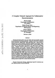
To establish a baseline, we generated ten validation areas, each with a radius of 1 km around a centroid that was selected randomly from the kernel density estimate of all vehicle activities as shown later in Figure 5a. Our area selection ensured that we would validate in areas where commercial activity would typically be high. Our choice of the number of validation areas, and the size of each area, although arbitrary, provided a set of areas with diverse activity densities and land uses. For each area we superimposed the vehicle activities on an aerial map of that area, and applied our judgement on which points should be clustered together to match the underlying land use. An example of one of the ten areas is shown in Figure 1. In Figure 1a we show the activity points, as
(a) Activities
(b) Clusters
Figure 1: To evaluate the clustering of activities into facilities, (1a) shows the clustering baseline identified through expert judgement; while (1b) shows an example of the clustering results and how the result is scored based on the baseline identified in (1a). Source: GoogleEarth at location 25°44’57.40”S, 28° 09’00.80”E, accessed on 10 December 2009. well as polygons representing our baseline of identified clusters. We note here that, due to the size and layout of large facilities such as shopping centres and distribution facilities with say H-shaped layouts, a number of independent clusters may make up a single facility. This has implications for later analysis. The baseline for each area v is the number, nv , and location of identified clusters. We denote the set of identified cluster, i.e. baseline clusters, in area v by B v . For each parameter combination = {", pmin } we execute the density-based clustering and compare the resulting clusters, denoted by R v , against the baseline clusters B v . Figure 1b shows one example of the resulting clusters (as spidergraphs) on top of the baseline clusters. A validation score, sv , made up of four penalty components, is then calculated for each area v and parameter combination . 1. Each baseline cluster b 2 B v not covered by any cluster r 2 R v , i.e. b \ R v = {·}, is penalised as a missed cluster. In Figure 1b there are two such instances. 2. Conversely, a fabricated cluster r 2 R v is one that is not associated with any b 2 B v , i.e. 6
r \ B v = {·}. Each fabricated point is penalised. This often occurs if pmin is set too low. In Figure 1b there is one instance, albeit on the periphery of the validation area. 3. If multiple clusters, say r1 , r2 , . . . , rm 2 R v , were identified in a single baseline cluster b 2 B v , we say that b has been split. Since only one of the m clusters would have been ideal, m 1 split penalty points are incurred. In Figure 1b there is only one such instance: a single baseline cluster covers m = 2 resulting clusters, and a split penalty of m 1 = 1 is incurred. 4. If multiple baseline clusters, say b1 , b2 , . . . , bn 2 B v were covered by a single resulting cluster r 2 R v , the baseline clusters are said to be merged. As for split clusters, a one-to-one match is sought, and a penalty of n 1 is incurred for each instance. In Figure 1b there are three instances, each merging two baseline clusters, so a penalty of 1+1+1=3 is incurred. The example in Figure 1b results in a total verification score of sv = 2 + 1 + 1 + 3 = 7. In an attempt to find the configuration with the lowest validation score, denoted ? , we identified four possible metrics to calculate (across all ten areas) for each combination : 1. average of the sum of scores, expressed as
1 10
2. average weighted sum of scores, expressed as
10 P
sv ;
v=1 1 10
10 P
v=1
sv nv ;
sv ; and v={1,...,10} n vo s 4. worst weighted score, expressed as max nv . 3. worst score, expressed as
max
v={1,...,10}
Validation was done for all the combinations of radii " = {10, 15, 20, 25, 30, 35, 40, 45} and minimum number of points pmin = {5, 10, 15, 20, 25, 30}. The results are visualised in Figure 2 with shades for each metric scaled between the worst (shaded black) and the best (shaded white) validation scores. The two extreme values are shown for each metric. The extreme values itself is of little importance. Of more importance is the configuration of " and pmin that yields the lower extreme value, shaded white. Although all metrics produce very similar result, we argue that using the maximum weighted score metric (Figure 2d) will yield robust clustering results that are best suited across a geographic area with diverse land uses, even more diverse than what we may have sampled. In the remainder of the paper, we used the search radius " = 30m and the minimum of pmin = 15 points suggested by Figure 2d in clustering the vehicle activities. The clustering algorithm was implemented in Java. Instead of considering clusters strictly within the province of Gauteng, we extended the study area (due to computational reasons) to be the bounding box of the province: the tightest rectangle that can be fitted around the extent of the province. A total of 43 477 facilities were identified in the study area. 4. Network analysis To establish a network among the facilities, we considered the detailed activity chains from the vehicles conducting the activities. As an illustration, consider the four activity chains in Figure 3a. From Joubert and Axhausen [20] we recall that major activities are those lasting in excess of five hours, representing depot locations where activity chains start and end. Although the example given in Figure 3a shows each chain starting and ending at the same major location, this need not be the case. Minor activities last less than five hours, and make up the various links in the activity chains. Of the twelve activity locations illustrated in the example, only nine were within the study area, of which seven were identified as facilities by the clustering algorithm and are included in our vertex 7
20
25
30
Radius (ε) 35
40
45
10
15
25
30
35
40
45
30
30
25
25
20
20
15
15
0.38
6
10
5
29
10
1.72
5
(a) Average sum of scores
Minimum number of points (pmin)
20
(b) Average weighted sum of scores
30
30
25
25
20
20
0.67
15
13
10
5
15
10
3.29
56 10
15
20
25
30
35
40
45
10
Radius (ε)
5
15
20
25
30
35
40
Radius (ε)
(c) Maximum score
(d) Maximum weighted score
Figure 2: Results from the cluster validation using four di↵erent metrics.
8
45
Minimum number of points (pmin)
Minimum number of points (pmin)
15
Minimum number of points (pmin)
Radius (ε) 10
V , E ) we consider the set V = {a, b, e, f, g, i, l}. To create the edge set, E , for our network graph G (V four vehicle chains, using a vehicle trip between two facilities, both contained in V , as the directed edge, or arc, connecting the facilities. The first chain, a ! b ! c ! d ! e ! a starts at facility a 2 V and proceeds to facility b 2 V . The trip originates at a, and so we increase the out-degree of a by one to keep track of the number of times a facility is the origin of an interaction. We also increase the in-degree of b by one as the trip terminates at b, keeping track of how many time each node is the destination of an interaction. Both a and b are within the study area; no network exists; so we establish a directed edge (dyad) between a and b and assign it a weight of one. Although the in- and out-degree can be calculated V , E ) directly, note that we keep a separate record of in- and out degrees. from the graph G = (V The reason for this is because not all activities in vehicle chains were identified as facilities, yet they remain activities nonetheless. For the next link in the activity chain, b ! c, we increase the out-order of b. Since c is not within the study area, c 3 V , its in-order is of no interest to us, and no edge is established. Link c ! d originates from outside the study area, so c’s out-degree is of no interest. Since d 3 V has not been identified as a facility, it is considered non-interesting and we don’t keep track of its in-degree, or create an edge between the two non-interesting facilities. Link d ! e originates at a non-interesting location, so d’s out-degree is of no interest, but the interaction terminates at facility e 2 V , so we increase the in-degree of e by one, and no edge is created between d and e. Link e ! a is again between two facilities in the vertex set, so we increase both the out-degree of e and the in-degree of a with one, and create an edge from e to a with weight one. The second chain, a ! b ! f ! g ! a, starts with a link from a 2 V to b 2 V , both facilities of interest, and we increase the out-degree of a and the in-degree of b by one. The edge from a to b already exists, so we increase its weight by one. We continue with links b ! f , f ! g and g ! a, increasing the out-degree of the origin and the in-degree of the destination by one in each case, and creating a directed edge with weight one between each pair. The third chain, k ! l ! k, only sees the in-degree and the out-degree of facility l 2 V increased by one, but no edges are created. The fourth chain’s first link, h ! i, will see facility i’s in-degree be increased by one. Although the facility is not strictly within the province, it is of interest since it is within the study area. Next, the out-degree of i and the in-degree of f will be increased by one, and we will create an edge from i to f . Since the next link, f ! j, originates at an interesting facility, f 2 V ’s out-degree will be increased, but no edge is created. Also, j 3 V ’s in-degree is of no interest. The link j ! h is also between non-interesting locations, so we discard the link. The adjacency matrix and the associated in- and out-degree values of the resulting weighted network for this illustration is given in Figure 3b. Of the possible 72 = 49 edges that may exist, only six entries exist, resulting in a density of 6/49 ⇡ 12.24%. Usually the degree of a facility is defined as the number of ties that a vertex has with other vertices in the network. The commercial vehicles we tracked perform activities across areas that exceed the study area, yet we were only interested in extracting the network as it exists within the study area. Hence we report, for example, a degree of 2 for facility l (sum of reported in- and out-degree) although the adjacency matrix reveals an order of 0 (sum of the number of row and column entries for l). This is valuable for later analysis. The complete vehicle data set from which activities were extracted contained 31,053 vehicles, representing approximately 1.5% of the national heavy and light delivery vehicle population. Of these vehicles, the complete network for Gauteng was established using the vehicle chains from 25,431 vehicles that travelled through, or conducted at least one activity within the study area. The network contained 43,477 facilities and 1,313,502 directed edges between facilities, resulting in a density of 0.06949%. In complex networks there is usually heterogeneity in the degree distribution, with some vertices 9
connected to very many other vertices, and others to only a few [27, 5, 34, 6, 28]. As LimaMendez and van Helden [25] suggest, one might be tempted to classify a complex network’s degree distribution, i.e. the number of connections a node has to other nodes in the network, as following a power law function. After fitting the function to the Gauteng network’s in-degree distribution (Figure 4a), we know this is not strictly the case. We also fitted a truncated power law function by considering a degree threshold, C ? , at which to split, i.e. truncate the data, fitting a separate power law function to each subset. On the x-axis of Figure 4a we plot the degree k, and on the y-axis the degree-distribution, p(k), indicating the number of vertices having a degree k. We estimated C ? =8 in Figure 4b with the resulting slope of the first section estimated as 1 = 0.846 with R2 =,0.9916, and the slope of the second section as 2 = -1.914 with R2 = 0.9201. The overall fit of the truncated power law had an R2 = 0.9212, compared to the much worse R2 = 0.8840 when only fitting a single power law function to the entire data set. The results were very similar for the out-degrees. The highest weight of any edge was 8,468, an average of more than 54 direct trips per day over the 6-month period (6 working days per week assumed). The 99th , 99.5th , 99.9th , 99.95th and 99.99th weight percentiles are 29, 47, 128, 203 and 533, respectively. 4.1. Identifying key facilities The notion of centrality is a key concept in network analysis, and relates to the relative importance of a facility due to its structural position in the network as a whole. Of interest to us is identifying who and where the central and/or important players in the network are. To identify the central actors in a network is useful since disseminating information such as policy or new technology, for example, will be best achieved when central actors are targeted. The conjecture in social network analysis is that the central node in a network can disseminate information fastest throughout the network. Since the central actors may be very difficult to identify due to the multiobjective nature of what makes an actor central, a number of centrality measures have been proposed to identify central and key actors, the latter being those that are most likely to be closely linked to central actors. A node’s betweenness centrality indicates on how many shortest paths between other nodes the node occur. Borgatti and Li [7] note that firms with high betweenness are structurally important to the economy itself, because if they disappear or become bottlenecks, they will a↵ect more other firms than if they had lower betweenness. The health of these facilities are important for the health of the rest of the network. The number of edges a node has within the network is referred to as its degree centrality. Well-connected nodes will score high on degree centrality, while nodes that are connected to wellconnected nodes may score high on a property known as eigenvalue centrality. Whereas a node’s degree centrality may be a proxy for the amount of information the node has, the eigenvalue centrality suggests that those that are connected to well-informed nodes may have access to more information than those nodes that are connected to an equal number, but less-informed nodes. To compare our network with other complete networks, our key network statistics are provided in Table 1 while Figure 5 provides the spatial distribution of the top 1000 ranked players in each of three centrality scores in subfigures (b) through (d). The eigenvalue centrality should be, in theory at least, an approximately linear function of the betweenness centrality. Any non-linear outliers will hence be facilities of interest. In Figure 6a we plotted the centrality scores with the transparency of each point representing the absolute size of the residual from the linear model fitted to the centrality scores of all 43 477 facilities. The more solid (darker) the point marker, the larger the absolute residual. The ten facilities with the highest absolute residuals are identified, and their geographic locations are shown in Figure 6b. With the exception of 143, 1364 and a lesser extent 8227, all facilities are rather centrally located and not 10
● ●
Clustered major location Clustered minor location Unclustered minor location Chain 1 Chain 2 Chain 3 Chain 4
c d e
a
To
b f
h
b
e
f
g
i
l
degree
a b e f g i l
– – 1 – 1 – –
2 – – – – – –
– – – – – – –
– 1 – – – 1 –
– – – 1 – – –
– – – – – – –
– – – – – – –
2 2 1 2 1 1 1
In-degree
2
2
1
2
1
1
1
i g j
From
l
k
bounding box
Out-
a
(a) Activity chains
(b) Resulting adjacency and degree matrix
Figure 3: Example illustrating the process of extracting a network graph from commercial vehicle activity chains.
R2= 0.9212 C* = 8 ● ●
3
10
●
Frequency
●
102
101
●●●●● ●● ●●● ● ● ● ● ● ● ● ● ● ● ● ● ● ● ● ● ● ●● ● ●● ●● ● ● ● ● ● ● ● ● ● ● ● ●● ● ● ● ● ● ● ● ● ●●● ● ●● ● ●● ● ●●● ● ● ● ●● ● ●● ●● ●●● ● ● ● ●● ● ● ●● ●●● ● ● ●● ●● ● ● ● ●● ● ● ●● ● ●●●● ●●●● ●●●● ● ●● ● ● ●●●● ● ● ●●●● ● ●● ●● ● ● ●● ● ● ●●●●● ●● ●● ● ● ●● ● ●●● ● ●● ● ● ●● ● ● ●● ● ●
● ●
0.92
● ●
●
● ● ●
●
0.91 ●
R2 ●
●
●
0.90 ●
● ●●● ●●● ● ●● ● ● ●● ● ●●● ●● ● ● ● ● ● ● ● ● ● ●● ● ●● ●●● ● ●
Observed values Power law Truncated power law
● ● ●● ● ● ● ● ● ● ● ● ● ● ● ● ●● ● ● ●●● ●●
●
0
10
●●●● ●● ● ● ● ● ● ● ● ● ● ● ● ● ● ● ● ● ● ● ● ● ● ● ● ● ● ● ● ● ● ● ●● ● ● ● ● ● ● ● ● ●●●●●
0.89 0
10
1
2
10
10
3
5
10
Degree
10
15 C
*
(b) Estimating C ? cuto↵
(a) Degree distribution
Figure 4: Determining the best fit function for the in-degree distribution. 11
●
0
12.5 25
Main freeways
50
75
100 Km
Zimbabwe
Rosslyn
Gauteng
Botswana Namibia
Pretoria
Krugersdorp
Minor activity density
Ekurhuleni Mozambique
Johannesburg
Vanderbijlpark Durban Cape Town
¸
(a) Reference map (Adapted from Joubert and Axhausen [20]).
(b) Weighted degree centrality
(c) Betweenness centrality
(d) Eigenvalue centrality
Figure 5: Spatial distribution of key players based on various centralisation scores. Size and transparency is related to the centrality score: the larger and more solid the marker, the higher the score.
12
Table 1: Network statistics. Percentile Mean a
Degree Degreeb Betweenness Eigenvalue
170.0 60.4 102477.5 1.89⇥10 3
21 16 0 0
Std dev
Min
651.4 128.4 969458.9 4.41⇥10 3
0 0 0 0
25
24 15 751 1.90⇥10 4
50th
75th
Max
44 26 4281 6.10⇥10 4
117 54 24004 1.76⇥10 3
34487 5796 90492630 1.51⇥10 1
Weighted by edge values. Not weighted.
Population (103)
515
Absolute value of residual ●
10−1
1.1601 x 10⁻¹ 8.7009 x 10⁻² 5.8006 x 10⁻² 2.9003 x 10⁻² 9.1379 x 10⁻⁸
2306 1364
666 500 333 167 0 Major highways ●
609
8232
7893
609
●
6133
ac
ce
ss
●
ue
7154
iq
●
●
Un
6133
●
515
8227
●
106
107
2306
7154
pe
tek ee 105
● ●
1364
●
143 ●
104
7893
rs
8232 143
10−2
Ga
b
Eigenvalue Centrality
a
Mode
th
8227
107
study area
Betweenness Centrality
(a)
(b)
Figure 6: Identifying key facilities as those with largest linear residuals.
13
on the periphery as might be expected. The majority of the facilities have close access to the main highways. The eight nodes with higher betweenness than eigenvalue centrality can be considered gatekeepers: having the capability for widespread interaction with other (especially central) facilities [12]. Why is this important? Gatekeepers are more likely to be well-informed stakeholders in policy planning. Identifying these facilities allow planners to target them with specific policy interventions—if it has economic and competitiveness improvement as its objective—potentially increasing the penetration and speed of e↵ect of such policy interventions in the industry. Of the seven identified gatekeepers, five were positively identified as depots and distribution centres of the same large brewery. We were unable to positively identify the other two. Introducing new technology such as radio-frequency (RF) consignment tracking, for example, requires large capital investments in infrastructure, but also operational process changes. Targeting gatekeeping facilities as entry points for new technology may increase the penetration and acceptance of the technology since gatekeepers are critical to central actors in the industry. The two facilities with higher eigenvalue centrality than betweenness, 1364 and 2306, are regarded as having unique access to central actors. If the direct identification of central actors remain elusive, targeting these facilities will likely yield access to central actors otherwise not achievable. Facility 1364 was identified as a large refuelling station on one of the major highways, while 2306—located close to the Johannesburg International Airport—was identified as an international distribution centre of industrial electronic components. Again, gaining access to central actors in the network allows for deeper and more rapid penetration of intervention, be it policy or technology. 4.2. Importers and exporters The in-degree of a facility is usually calculated as the column sum of ties that exist in the adjacency matrix for the facility. Only arrivals from other facilities within the network are thus considered. Similarly, the out-degree is calculated as the row sum of existing ties. However, earlier in this section we noted that we captured the in-degree of a facility as the total number of times that the facility was the destination of an interaction, whether the interaction originated from a facility within the network or from outside. Similarly, the out-degree is the number of times that the facility was the origin of an interaction, irrespective of whether the destination was within or outside the study area. In the absence of any further information, we do not know which interaction of a vehicle with a facility is important: if it arrives at the facility with a delivery and leave empty, we might argue that the in-degree is actually worthy of our consideration. Or, if the vehicle arrived empty or partially laden to collect, and leave loaded, we might argue that the out-degree is of more importance. Unfortunately we do not have any additional information with regards to what the purpose of the interaction is. For each activity then, both the arrival and the departure are captured in the inand out-degree values respectively, yielding them essentially equal. An analytical opportunity arises when the two ways of defining in- and out-degrees are combined. For this purpose we will refer to both our in- and out-degree values, since they are the same, as d? , and to the more classic approach as din and dout , respectively. The di↵erence, d? din , then indicates how many more external than internal interactions a facility had as destination. A high value indicates a facility that receives more vehicles from outside the study area. Similarly, a high value obtained for the di↵erence d? dout indicates a facility from where a large number of vehicles depart to destinations outside the study area. For an economy with balanced imports and exports the two di↵erences should be approximately linear. In Figure 7 we plot the two di↵erences against one another, and indicate with the transparency of the markers again the absolute residuals from the fitted linear model. There is visibly 14
2000 Absolute value of residual 104
7500 5000 2500 0
666 500 333 167 0
2777
Major highways
609
1549
●
414
414
et
ex p
1999
42 361
Population (103)
609
N
Difference in out−order
or
te
r
●
515
●
103
2000
●
454
515
2777 1549 454 ●
● ●
●
●
●
1999
361
po
rte
r
●
42
N
et
im
102
102
103
104
study area
Difference in in−order
(a)
(b)
Figure 7: Identifying key net importers and exporters as those with largest linear residuals. more net exporters in Gauteng than importers. As we have for the identification of key actors, we identify the top ten facilities in terms of the size of the absolute residuals. This analysis is useful in identifying the key importers and exporters in the province. From Figure 7a there does not seem to be a clear break between the lower left quadrant and the upper right quadrant to distinguish between internally focused, and externally focused facilities. From Figure 7b we see that key importers and exporters are in close proximity to the main highways. Since facilities 42, 1999 and 2000 are outside the province we have little interest in them. Four of the eight net exporters were fuelling stations. Facilities 42, 361 and 414 were all retailer refuelling stations located on major highways, while facility 1549 was identified as a wholesale diesel outlet close to the Johannesburg International Airport. It makes intuitive sense that many vehicles refuel before embarking on distant journeys elsewhere in the country. Unfortunately we were unable to positively identify facility 515 in the central business district of Johannesburg, or facility 2000. Of the two importers, facility 454 is a distribution centre of a large broiler operator: importing frozen poultry products from the Western Cape. The other, 2777, is located close to the international airport and is the distribution centre for industrial bearings and components. One may question the usefulness of identifying refuelling facilities. In some settings, we agree, it may have little value. But if one considers locations to put vehicle weight monitoring and enforcement infrastructure, you definitely should consider refuelling facilities given their prominence in the network. Also, when simulating activity chains, they clearly make up a noticeable portion of the activities and should thus be included if one aims to duplicate reality. With the exception of facilities 414 and 361, it is a concern that the majority of the key importers and exporters are not located closer to the periphery of the urban areas. Joubert and Axhausen [20] note that the omnidirectional through-traffic makes Gauteng an obvious choice as a hub connecting the two main ports from the South-East (Durban) and South-West (Cape Town) with the northern 15
neighbours. If the importing and exporting of goods remain, which are economically beneficial, the transport planning challenge is to ensure flow on the main freeways, especially in the urban centres. Using commercial vehicle activities and the associated network analysis approach is very useful to identify the key importing and exporting facilities. It allows transport planners and provincial and local governments to derive directed and specific policy measures. Our methodology can help identify key stakeholders to involve in designing, testing and implementing policy instruments such as concessionary real estate rates or construction and relocation subsidies that may ensure enhanced competitiveness for the facilities, and indirectly improve congestion in the urban centres if some of the key importers and exporters do decide to relocate more towards the urban periphery. Since large refuelling stations seem to be the last port-of-call for many vehicles, they may be useful locations to consider the placement of weigh-in-motion facilities to police and enforce vehicle (especially heavy vehicle) axle overloading. 4.3. Cohesive subgroups We argue that it is beneficial for firms that facilities that are connected with weighty ties should be located close together, lowering logistic costs. If combined with shared services and accessible location choice, as is the case in supplier parks and industrial zones, other economic benefits may also arise. Urban economics refers to such benefits as economies of agglomeration. Further benefits related to knowledge di↵usion and organisational growth has also been studied [10, 11]. We wanted to investigate whether firms with high volumes of inter-facility flows are indeed located in close proximity within Gauteng, and also where they are located. If facilities are dispersed, our analysis would be useful in identifying opportunities where firms can consider the benefits of relocating into industrial districts to reap economic benefits. Within such cohesive subgroups, or small economies, various opportunities for load consolidation may be identified, or empty legs of activity chains might be reduced. To identify such small economies, we reduced the original network into weak components. A weak component is a subgraph in which all nodes (facilities) are connected with at least one edge, in either direction. To extract the weak components we removed all directed ties with weight less than 200 (approximately the 99.95th percentile); and removing all resulting isolates (unconnected facilities). The resulting network components are illustrated in Figure 8a. We’ve plotted the directed graphs of selected components from Figure 8a over the population densities in Figure 8b. At first glance of Figure 8a one notices the large proportion of components (65%) that only contains 2 facilities; and those containing 3 facilities (15%). Borgatti and Li [7] suggest that such isolated components is often the result of e↵ective links (business transactions) that drifted o↵ to become independent. In the context of this paper one should be careful to infer too much from such a suggestion: Many of the two-node components are often two positions at the same, albeit very large, facility that could not be jointly identified during clustering. One may be tempted to ask: “why not then change the clustering parameters?” The answer may be given through an example: a large commercial facility like a shopping mall may be identified as two separate clusters, one at the receiving docks at the back of the facility, and the other in the parking area in front. These two facilities may represent the same complex, but are quite di↵erent in function. Similarly, a large distribution centre may have its receiving and despatch areas identified as di↵erent facilities by the clustering algorithm, but again it is arguable that the two areas should be considered separately based on the functions performed at each. If a vehicle then moves from one facility to another at the same business complex, it may in fact be doing so to perform a specific, yet di↵erent function than at the first. For this reason we do not want to merely change the clustering parameters to avoid these occurrences, or artificially merge them postmortem. 16
Edge weight 8500 6450 4350 2250 200
Number of trips 8500 6450 4350 2250 200
c1
Population (103) 666 500 333 167 0
c1
● ● ● ● ●
●
● ●
●
c6 c6
●● ● ● ● ●
● ● ●
● ● ●
●
c5
c2
c4
●
●
c5
●● ● ● ●● ● ● ● ● ● ●
● ●●
● ●● ● ●
● ●
● ●
c2
●● ● ●● ● ● ●● ● ● ● ● ● ● ●●● ● ● ●● ● ●●● ●
● ● ● ●● ● ●● ● ● ● ●● ● ● ●● ●● ● ● ● ●●●● ● ● ●
● ● ● ● ● ● ● ● ● ● ● ●
●
● ●● ● ● ●
●
c3
c3
●● ● ●● ● ●●
● ● ●●
0
c4
(a) The social network graph.
10
20
30
40
Km
study area
(b) Identified components plotted at their geographical locations in the study area.
Figure 8: Cohesive subgroups extracted from the original network. Each component can be considered a small economy since the facilities have frequent direct interaction. Some components in (a) are selected based on the edge weights. The selected components are located accordingly in (b).
17
We tried to, in the absence of additional land use information, derive the likely business of each of the components using address searches and aerial photographs. We also report on the approximate number of vehicle kilometres (vkm) travelled in each component, using the number of trips and the Euclidean distance between the facilities. Component c1 contains 15,390 trips and accounts for 160,081 vkm (an average of 1026 vkm per day). As was the case with gatekeepers, c1 is dominated by the brewery’s depots and distributions centres. Component c2 contains 69,666 trips and accounts for 314,286 vkm (2015 vkm per day); is located outside of the province; and is related to coal-mining, linking collieries with processing facilities. Component c3 contains 15,614 trips, accounts for 166,074 vkm (1065 vkm per day) and is construction-related, linking various cement factories and depots to facilities which seem like retail construction material and do-it-yourself supply outlets. We were not able to distinctly identify the businesses in c4 which contains 10,373 trips and accounts for 25,552 vkm (164 vkm per day), although it is likely to be associated with the textile production industry. Component c5 contains 46,720 trips and accounts for 409,750 vkm (2627 vkm per day). While the various parts of component c5 seem unrelated, they are linked by a few truck rental depots. We argue that although the business may not be related, they all make use of outsourced fleets for their transportation needs. A number of large industrial manufacturing plants and distribution centres are also present in c5 . The majority of facilities in c6 , containing 17,610 trips and accounting for 91,199 vkm (585 vkm per day), are located near or at the freight terminal of the Johannesburg International Airport, while a small number of other facilities seem to be either small storage and distribution centres, or manufacturing plants. In Figure 8b we notice that the number of trips are dominated by c2 . At the given scale the distances travelled seem negligible, yet varied between 171m (travelled 374 times) and 30.9km (travelled 447 times). One can conclude that c2 is a small economy well positioned: facilities are close to one another; and vehicle movement does not seem to interfere with high population densities. The nature of the business, however, usually sees mining and processing operations located close to one another. The positioning of c2 is in contrast with that of c1 and c3 through c6 where frequent trips are conducted over larger distances, most notably 27.8 km for c1 (2262 times); 55.1 km for c3 (531 times); 9.6 km for c4 (783 times); 20.1 km for c5 (856 times), and 12.8 km for c6 (2701 times). Of concern, with the exception of c2 again, is the proximity of the highest activity components to the densely populated areas. This is further confirmation of Joubert and Axhausen [20] where competition for land exist between industry and especially the low-income portion of the population. Being able to identify and subsequently rank the cohesive subgroups, urban and transport planners may identify easy wins if policy instruments are targeted towards the high-ranked components. Opportunities exist to jointly improve the logistic state-of-a↵airs for the small economic components, and at the same time addressing mobility in the urban centres, assuming the relocation of the components are considered viable. 4.4. Implications for transport planning Much of our application of network analysis so far has had a strong link with economic policy and regional science. The link between transport and economic performance is well-established [4]. In this section we give two examples on using network analysis more specifically in transport planning. Having a network graph allows one an array of analysis [5]. Other than just the graph’s topology, spatial networks has implications for transport such as distance and cost. When coupled with observed activity chains, such as those described by Joubert and Axhausen [20], one can find similarities between di↵erent vehicles’ trajectories (chains) of the graph [36]. Such similar paths highlights corridors of activity more accurately than just vehicle counts. Travel demand management measures such as road pricing, load consolidation, and road space reallocation may be directed at 18
these corridors. Coupling the activity chains with the graph also provides the ability to identify those facilities where the diversity of di↵erent vehicles are higher. If only vehicle volumes are used to identify locations for vehicle weight enforcement one stands the chance to monitor too small a subset of the vehicle population. The second use of the network relates to transport modelling. Recent developments in agentbased transport favoured private cars and individuals, while Liedtke [24], Joubert et al [21] and Schr¨oder et al [32] specifically addressed freight vehicles. For such models, an initial activity chain is required for each agent. In the context of this paper, agents refer to commercial vehicles and a vehicle’s activity chain represents the sequence of activities the vehicle will execute in the mobility simulation. Sampling from a weighted directed network, as we’ve created in this paper, allows the transport modeller to create synthetic activity chains that accurately reflect reality. To illustrate the generation of an activity chain, consider the weighted network given in Figure 9 that assumes three di↵erent weights: one, two and three. From Joubert and Axhausen [20] one can sample the start time, duration, and number of activities per chain. The first activity, say a, can be sampled from a kernel density estimate as provided in Figure 5. If one wants to create a synthetic activity chain with n activities, the sequence of activities is best sampled from the weighted network using a Monte Carlo method. All the outgoing edges of an activity is taken and its weighted probability is used for sampling the next activity location. The probability that activity
Figure 9: An example of a weighted network with three di↵erent dyad weights: one, two and three. 2 a is followed by activity b is 2+1+3+1 = 27 ⇡ 29%. Similarly, the probabilities that a is followed by c is 17 ⇡ 14%; by d, 37 ⇡ 43%; and by e, 17 ⇡ 14%. Say b is chosen randomly as the activity following a. All the outgoing edges of b is then considered, and the next activity might be c, with probablity 2 2 3 2+3 = 5 = 40%, or d, with probability 5 = 60%. Say d is chosen, then the next activity might be 2 a, with probability 2+1+2 = 25 = 40%, b, with probability 15 = 20%, or e, with probability 25 = 40%. The process is repeated until n 1 activities have been sampled, and the last activity location is then the same as the first. Alternatively, if the start and end locations need not be the same, the process is repeated n times as opposed to n 1 times. Using the weighted network to sample activity sequences promises to be more accurate than sampling n activities, in random sequence, from the kernel density estimate directly. Modelling commercial vehicles more accurately and realistically results in more accurate predictions of travel time, for example. Both Gao et al [9] and Fourie [8] show how agent-based models are more realistic in predicting travel times. When testing infrastructure investment decisions, say the
19
expansion of a portion of the road network, improved travel time prediction allows better evaluation of the direct e↵ects (travel time savings) of the investment. 5. Conclusion With this paper we’ve taken a step in linking the complex network among players in the supply chain domain with transport planning. To achieve this, we used the movement of commercial vehicles between facilities as a proxy for the directed edges in a weighted network. Such an approach has both positive and negative consequences. On the up-side, we were able to extract a very large complex network among facilities. Applying network analysis allowed us to make useful and novel discoveries about the relationships among, and locations of the key facilities. We argue that involving these key players in policy making will allow government to develop targeted instruments that will better both the economic position of the stakeholders, and the mobility and level of congestion of the urban centres. Towards the down-side we acknowledge that the current approach, in the absence of any additional information about the trip purposes that we used as proxy, may yield or strengthen social relationships between facilities that were actually merely incidental. From Joubert and Axhausen [20] we know that vehicle chains often contain as many as 25 activities per chain. It is therefore plausible to consider two consecutive facilities in a chain merely incidental; the result of some route optimisation performed by a logistics service provider’s scheduler. Further trip-specific information will be needed to refine the purpose of each network edge. We are closer in contributing towards the work started by Liedtke [24], Schr¨ oder et al [32] and others to predict vehicle movement from the ‘social’, i.e. supply chain networks. It is our belief that the process followed in this paper remain valid and novel to demonstrate the extent and location of interactions; identify key players; and yield valuable characteristics about players. The way in which we extracted high-activity components, for example, can yield opportunities for companies seeking to identify partners with whom they can pursue load consolidation and fleet optimisation benefits. When accompanied with targeted policy instruments, firms may relocate jointly into more clustered environments such as industrial development zones or supplier parks and reap logistic cost benefits, as well as economic benefits from shared services and knowledge exchange. To evaluate the extent of economic benefits for such a component one would have to extract a more detailed network for the specific component. Barth´elemy [5] rightfully indicates that space is relevant in many networks, particularly distance (and associated costs) in transportation networks. One branch of future research is to better understand how the topological aspects of the network as we’ve introduced in this paper correlate to spatial aspects such as the location of facilities, and the length of trips between them. Another branch of research to pursue is the analysis of commercial vehicle activity chains to find similarity in its network trajectories [36]. Such similarities would allow transport planners to generate/simulate activity chains from spatial networks. Acknowledgements Thank you to the anonymous reviewers for their valuable feedback and review comments. The first author is grateful to the South African National Research Foundation (NRF) for funding the research under Grant FA-2007051100019; and also to the University of Pretoria’s Research Development Programme. All figures except Figure 9 were created using R [30]. [1] Albert R, Jeong H, Barab´ asi AL (2000) Error and attack tolerance of complex networks. Nature 406:378–382 20
[2] Andrienko G, Andrienko N, Bak P, Keim D, Kisilevich S, Wrobel S (2011) A conceptual framework and taxonomy of techniques for analyzing movement. Journal of Visual Languages and Computing 22(3):213–232 [3] Autry CW, Griffis SE (2008) Supply chain capital: The impact of structural and relational linkages on firm execution and innovation. Journal of Business Logistics 29(1):157–173 [4] Banister D, Berechman Y (2001) Transport investment and the promotion of economic growth. Journal of Transport Geography 9(3):209–218 [5] Barth´elemy M (2011) Spatial networks. Physics Reports 499(1–3):1–101 [6] Boccaletti S, Latora V, Moreno Y, Chavez M, Hwang DU (2006) Complex networks: Structure and dynamics. Physics Reports 424(4–5):175–308 [7] Borgatti SR, Li X (2009) On social network analysis in a supply chain context. Journal of Supply Chain Management 45(2):5–22 [8] Fourie P (2010) Agent-Based transport simulation versus equilibrium assignment for private vehicle traffic in Gauteng. In: 29th Annual Southern African Transport Conference, 12–23. [9] Gao W, Balmer M, Miller EJ (2009) Comparison of MATSim and EMME/2 on greater Toronto and Hamilton area network, Canada. Transportation Research Record 2197:118–128 [10] Giuliani E, Bell M (2005) The micro-determinants of meso-level learning and innovation: evidence from a chilean wine cluster. Research Policy 34(1):47–68 [11] Giuliani E, Pietrobelli C, Rabellotti R (2005) Upgrading in global value chains: Lessons from latin american clusters. World Development 33(4):549–573 [12] Graf H, Kr¨ uger JJ (2009) The performance of gatekeepers in innovator networks. Jena Economic Research Papers in Economics 2009-058, Jena, Max-Planck-Institute of Economics, [13] Hackney JK, Marchal F (2009) A model for coupling multi-agent social interactions and traffic simulation. In: 88th Annual Meeting of the Transport Research Board [14] Halkidi M, Batistakis Y, Vazirgiannis M (2001) On clustering validation techniques. Journal of Intelligent Information Systems 17(2):107–145 [15] Hensher D, Figliozzi MA (2007) Behavioural insights into the modelling of freight transportation and distribution systems. Transportation Research Part B: Methodological 41(9):921–923 [16] Hensher DA (2007) Models of organizational and agency choices for passenger- and freightrelated travel: Notions of interactivity and influence. In: Axhausen KW (ed) Moving Through Nets: The Physical and Social Dimensions of Travel, Elsevier, Amsterdam, pp 107–130 [17] Hesse M, Rodrigue J (2004) The transport geography of logistics and freight distribution. Journal of Transport Geography 12(3):171–184, [18] Holme P, Kim BJ, Yoon CN, Han SK (2002) Attack vulnerability of complex networks. Physical Review 65(056109):1–14 [19] Jain AK, Murty MN, Flynn PJ (1999) Data clustering: a review. ACM Computing Surveys 31(3):264–323 21
[20] Joubert JW, Axhausen KW (2011) Inferring commercial vehicle activities in Gauteng, South Africa. Journal of Transport Geography 19(1):115–124, [21] Joubert JW, Fourie PJ, Axhausen KW (2010) Large-scale agent-based combined traffic simulation of private cars and commercial vehicles. Transportation Research Record 2168:24–32 [22] Kowald M, Frei A, Hackney JK, Illenberger J, Axhausen KW (2009) Collecting data on leisure travel: The link between leisure acquaintances and social interactions. In: Applications of Social Network Analysis [23] Lazzarini S, Chaddad F, Cook M (2001) Integrating supply chain and network analyses: The study of netchains. Journal on Chain and Network Science 1(1):7–22 [24] Liedtke G (2009) Principles of micro-behavior commodity transport modeling. Transportation Research Part E: Logistics and Transportation Review 45(5):795–809 [25] Lima-Mendez G, van Helden J (2009) The powerful law of the power law and other myths in network biology. Molecular BioSystems 5(12):1482–1493 [26] Nanni M, Pedreschi D (2006) Time-focused clustering of trajectories of moving objects. Journal of Intelligent Information Systems 27(3):267–289 [27] Newman MEJ (2003) The structure and function of complex networks. SIAM Review 45(2):167–256 [28] Newman MEJ (2005) Power laws, pareto distributions and zipf’s law. Contemporary Physics 46(5):323–351 [29] Pelekis N, Kopanakis I, Kotsifakos EE, Frentzos E, Theodoridis Y (2011) Clustering uncertain trajectories. Knowledge and Information Systems 28(1):117–147 [30] R Core Team (2012) R: A Language and Environment for Statistical Computing. R Foundation for Statistical Computing, Vienna, Austria, http://www.R-project.org/, ISBN 3-900051-070 [31] Roorda MJ, Cavalcante R, McCabe S, Kwan H (2010) A conceptual framework for agent-based modelling of logistics services. Transportation Research Part E: Logistics and Transportation Review 46(1):18–31 [32] Schr¨oder S, Zilske M, Liedtke GT, Nagel K (2012) Computational framework for multiagent simulation of freight transport activities. In: 91st Annual Meeting of the Transportation Research Board, Paper 12-4152 [33] Spaccapietra S, Parentb C, Damiania ML, de Macedoa JA, Portoa F, Vangenota C (2008) A conceptual view on trajectories. Data & Knowledge Engineering 65(1):126–146 [34] Strogatz SH (2001) Exploring complex networks. Nature 410:268–276 [35] Theodoridis S, Koutroumbas K (2006) Pattern Recognition, 3rd edn. Academic Press [36] Tiakas E, Papadopoulos A, Nanopoulos A, Manolopoulos Y, Stojanovic D, Djordjevic-Kajan S (2009) Searching for similar trajectories in spatial networks. The Journal of Systems and Software 82(5):772–788 22
[37] Zhou C, Frankowski D, Ludford P, Shekhar S, Terveen L (2004) Discovering personal gazetteers: an interactive clustering approach. In: Proceedings of the 12th annual ACM international workshop on Geographic Information Systems, ACM, Washington DC, USA, pp 266–273
23