Oct 2, 2015 - a user and BPI be the set of top t best predicted items for the user. BCR ..... [6] Michael D Ekstrand, John T Riedl, and Joseph A Konstan.
arXiv:1510.00585v1 [cs.IR] 2 Oct 2015
A Complex Network Approach for Collaborative Recommendation Ranveer Singh Department of Mathematics IIT Jodhpur Bidyut Kumar Patra Department of Computer Science and Engineering NIT Rourkela Bibhas Adhikari Department of Mathematics IIT Kharagpur October 5, 2015 Abstract Collaborative filtering (CF) is the most widely used and successful approach for personalized service recommendations. Among the collaborative recommendation approaches, neighborhood based approaches enjoy a huge amount of popularity, due to their simplicity, justifiability, efficiency and stability. Neighborhood based collaborative filtering approach finds K nearest neighbors to an active user or K most similar rated items to the target item for recommendation. Traditional similarity measures use ratings of co-rated items to find similarity between a pair of users. Therefore, traditional similarity measures cannot compute effective neighbors in sparse dataset. In this paper, we propose a two-phase approach, which generates user-user and item-item networks using traditional similarity measures in the first phase. In the second phase, two hybrid approaches HB1, HB2, which utilize structural similarity of both the network for finding K nearest neighbors and K most similar items to a target items are introduced. To show effectiveness of the measures, we compared performances of neighborhood based CFs using state-of-the-art similarity measures with our proposed structural similarity measures based CFs. Recommendation results on a set of real data show that proposed measures based CFs outperform existing measures based CFs in various evaluation metrics.
Keyword- Collaborative filtering, neighborhood based CF, similarity measure, sparsity problem, structural similarity.
1
1
Introduction
In the era of information age, recommender systems (RS) has been established as an effective tool in various domains such as e-commerce, digital library, electronic media, on-line advertising, etc. [20][2][14][11]. The recommender systems provide personalized suggestions about products or services to individual user filtering through large product or item space. The most successful and widely accepted recommendation technique is collaborative filtering (CF), which utilizes only user-item interaction for providing recommendation unlike content based approach [13] [17]. The CF technique is based on the intuition that users who has expressed similar interest earlier will have alike choice in future also. The approaches in CF can be classified into two major categories, viz. model based CF and neighborhood based CF. Model-based CF algorithms learn a model from the training data and subsequently, the model is utilized for recommendations [21][18][8]. Main advantage of the model-based approach is that it does not need to access whole rating data once model is built. Few model based approaches provide more accurate results than neighborhood based CF [12][6]. However, most of the electronic retailers such as Amazon, Netflix deployed neighborhood based recommender systems to help out their customers. This is due to the fact that neighborhood based approach is simple, intuitive and it does not have learning phase so it can provide immediate response to new user after receiving upon her feedback. Neighborhood based collaborative algorithms are further classified into two categories, viz. user based and item based CF. The user based CF is based on a principle that an item might be interesting to an active user in future if a set of neighbors of the active user have appreciated the item. In item based CF, an item is recommended to an active user if she has appreciated similar items in past. N eighborhood based CF recommendation extracts user-user or item-item similarity generally using Pearson Correlation Coefficient(PCC)and its variants, slope-one predictor from user-item matrix to predict rating of user for new item [9]. Item based CF is preferred over user based CF if number of items is smaller in number compared to the number of users in the system. Generally, neighborhood based CF uses a similarity measure for finding neighbors of an active user or finding similar items to the candidate item. Traditional similarity measures such as pearson correlation coefficient, cosine similarity and their variants are frequently used for computing similarity between a pair of users or between a pair of items [5]. In these measures, similarity between a pair of users is computed based on the ratings made by both users on the common items (co-rated item). Likewise, item similarity is computed using the ratings provided by users who rated both the items. However, correlation based measures perform poorly if there are no sufficient numbers of co-rated items in a given rating data. Therefore, correlation based measure and its variants are not suitable in a sparse data in which number of ratings by individual user is less and number of co-rated items is few or none [10]. In this paper, we propose a novel approach for computing similarity between a pair of users (items) in sparse data. In the proposed approach, a user-user (item-item) network is generated using pearson correlation (adjusted cosine) for computing similarity between a pair of users (items). Having generated the net2
works, we exploit the structures of the network for addressing few drawbacks of neighborhood based CF. Having generated the networks, we exploit the structures of the network for computing similarity in sparse data and predictions for an item which receives ratings from few users. The approach is tested on real rating datasets. The contributions in this paper are summarized as follow. • We propose a novel approach to utilize traditional similarity measures to generate user-user and item-item networks. The generated networks help in establishing transitive interaction between a pair of users, which is difficult to capture using traditional measures. • The user based CF fails to predict rating of an item if it receives rating from few users (less than K users). Structure of the networks are exploited to address this problem by combining item based CF with the user based CF. Two algorithms termed as HB1 and HB2 are introduced for this purpose. • We discuss the drawback of the use of F1 measure in recommendation scenario and introduce a new metric to evaluate qualitative performance of the collaborative filtering algorithms to capture the variation of rating provided by individual user. • To show the effectiveness of the proposed approach in sparse dataset, we implemented neighborhood based CF using traditional similarity measures and neighborhood based CF using proposed approach. The rest of the paper is organized as follows. The background and related research are discussed in Section 2. The proposed novel approach is introduced in Section 3. Experimental results and evaluation of the proposed approach are reported in Section 4. We conclude the paper in Section 5.
2
Background and related work
In this section, we discuss working principle of neighborhood based approach in detail and different similarity measures introduced in literature in-order to increase performance of recommendation systems over past decades.
2.1
Neighborhood-Based Approach
The neighborhood or memory based approach is introduced in the GroupLens Usenet article[19] recommender and has gained popularity due to its wide application in commercial domain [14][3][1]. This approach uses the entire rating dataset to generate a prediction for an item (product) or a list of recommended items for an active user. Let R = (rui )M×N be a given rating matrix (dataset) in a CF based recommender system, where each entry rui represents a rating value made by uth user Uu on ith item Ii . Generally, rating values are integers within a rating domain(RD), e.g 1-5 in MovieLens dataset. An entry rui = 0 indicates user Uu has not rated the item Ii . The prediction task of neighborhood-based CF algorithm is to predict rating of the ith item either using the neighborhood information of uth user (user-based method) or using neighborhood information of ith item (item-based method). 3
Neighborhood-based Prediction method can be divided into two parts Userbased and Item-based. User based methods predicts based upon on ratings of ith item made by the neighbors of the uth user [5][7]. This method will computes similarity of the active user Uu to other users Up ,p = 1, 2...M, p 6= u. Then K closest users are selected to form neighborhood of the active user. Finally, it predicts a rating rˆui of the ith item using the following equation. rˆui = r¯u +
PK
s(Uu , Uk )(rki − r¯k ) PK k=1 |s(Uu , Uk )|
k=1
(1)
where, r¯u is the average of the ratings made by user Uu . s(Uu , Uk ) denotes similarity value between user Uu and its k th neighbor. r¯k is the average of ratings made by k th neighbor of the user Uu , and rki is the rating made by k th neighbor on ith item. Item-based collaborative filtering [14] has been deployed by world’s largest online retailer Amazon Inc [14]. It computes similarity between target item Ii and all other items Ij , j = 1, ...N i 6= j to find K most similar items. Finally, unknown rating rˆui is predicted using the ratings on these K items made by the active user Uu . rˆui = r¯i +
PK
s(Ii , Ik )(ruk − r¯k ) PK k=1 |s(Ii , Ik )|
k=1
(2)
where, r¯i is the average of the ratings made by all users on items Ii , s(Ii , Ik ) denotes the similarity between the target item Ii and the k th similar item, and ruk is the rating made by the active user on the k th similar item of Ii . Similarity computation is a vital step in the neighborhood based collaborative filtering. Many similarity measures have been introduced in various domains such as machine learning, information retrieval, statistics, etc. Researchers and practitioners in recommender system community used them directly or invented new similarity measure to suit the purpose. We discuss them briefly next.
2.2
Similarity Measures in CF
Traditional measures such as pearson correlation coefficient (PC), cosine similarity are frequently used in recommendation systems. The cosine similarity is very popular measure in information retrieval domain. To compute similarity between two users U and V , they are considered as the two rating vectors of n dimensions, i.e., U, V ∈ N0n , where N0 is the set of natural numbers including 0. Then, similarity value between two users is the cosine of the angle between U and V . Cosine similarity is popular in item based CF. However, cosine similarity does not consider the different rating scales (ranges) provided by the individual user while computing similarity between a pair of items. Adjusted cosine similarity measure addresses this drawback by subtracting the corresponding user average from the rating of the item. It computes linear correlation between ratings of the two items. Pearson correlation coefficient (PCC) is very popular measure in user-based collaborative filtering. The PCC measures how two users (items) are linearly related to each other. Having identified co-rated items between users U and V , PCC computes correlation between them [4]. The value of PCC ranges in [−1
4
+1], The value +1 indicates highly correlated and −1 indicates negatively corelated to each other. Likewise, similarity between two items I and J can also be computed using PCC. Constrained Pearson correlation coefficient (CPCC) is a variant of PCC in which an absolute reference (median in the rating scale) is used instead of corresponding user’s rating average. Jaccard only considers the number of common ratings between two users. The basic idea is that users are more similar if they have more common ratings. Though profoundly used PCC and its variants suffer from some serious drawbacks described in section 4. PIP is the most popular (cited) measure after traditional similarity measures in RS. The PIP measure captures three important aspects (factors) namely, proximity, impact and popularity between a pair of ratings on the same item [4]. The proximity factor is the simple arithmetic difference between two ratings on an item with an option of imposing penalty if they disagree in ratings. The agreement (disagreement) is decided with respect to an absolute reference, i.e., median of the rating scale. The impact factor shows how strongly an item is preferred or disliked by users. It imposes penalty if ratings are not in the same side of the median. Popularity factor gives important to a rating which is far away from the item’s average rating. This factor captures global information of the concerned item. The PIP computes these three factors between each pair of co-rated items. PIP based CF outperforms correlation based CF in providing recommendations to the new users. Haifeng Liu et al. introduced a new similarity measure called NHSM (new heuristic similarity model), which addresses the drawbacks of PIP based measure recently. They put an argument that PIP based measure unnecessarily penalizes more than once while computing proximity and impact factors. They adopted a non-linear function for computing three factors, namely, proximity,significance, singularity in the same line of PIP based measure. Finally, these factors are combined with modified Jaccard similarity measure [15]. Koen Verstrepen and Bart Goethals proposed a method that unifies userand item based similarity algorithms [22], but it is suitable for binary scale. Before proposing our method, let us first analysis the problem with methods which use co-rated items through experiments on different datasets. These problems motivated us to formulate our proposed methods.
3
Proposed method for rating prediction
As mentioned earlier, we employ the well developed concept of similarities of nodes in a network for the prediction of entries of a rating matrix when a network is generated by using the given data. We propose to generate an user-user (resp. item-item) weighted network with node set as the set of users (resp. items) and the links in the network are defined by the PCC similarity of the users (resp. items) in the given data. Once the network is generated, a local similarity metric for nodes reveals insights about the connectivity structure of neighbors of a given node, and a global similarity metric provides the understanding of how a node is correlated with rest of the nodes in the network. Thus, a network approach to determine correlations between users or items provides a holistic outlook into the interpretation of a data. Further, in order to reduce sparsity in the data for rating prediction, we introduce the concept of intermediate rating for an item by an user who has not
5
rated the corresponding item. Thus, we use both the user-user and item-item network structural similarities to propose new metrics for rating prediction.
3.1
Network generation and structural similarities
Let U and I denote the set of users and items respectively of a given data set. The adjacency matrix A = [Aij ] for the user-user (resp. item-item) weighted network is defined by Ai,j = PCC(i, j) where i, j denote users (resp. items) and PCC(i, j) denotes the PCC similarity between ith and jth nodes. Thus, in the user-user (resp. item-item) network, the users (resp. items) are represented by nodes and links between any two nodes are assigned with weight PCC(i, j) if PCC(i, j) 6= 0 otherwise the nodes are not linked. The size of the user-user (resp. item-item) network is given by |U| (resp. |I|) where |X| denotes the carnality of a set X. In this paper, we consider the following structural similarities for the useruser or item-item network. Let A denote the adjacency matrix associated a network G. For a node i of G, let γ(i) denote the set of neighbors of i. • Common Neighbors (CN)[16]. The CN similarity of two distinct nodes i and j is defined by sCN = |γ(i) ∩ γ(j)|. ij It is obvious that sCN = [A2 ]ij , the number of different paths with length ij 2 connecting i and j. So, more the number of common neighbors between two nodes, more is the value sCN between them. ij • Jaccard Similarity [16]: This index was proposed by Jaccard over a hundred years ago, and is defined as sJaccard = ij
|γ(i) ∩ γ(j)| |γ(i) ∪ γ(j)|
for any two distinct nodes i and j in the network. • Katz Similarity [16]. The Katz similarity of two distinct nodes i, j is defined by sKatz = ij
∞ X
β l · |paths < l >ij | = βAij + β 2 [A2 ]ij + β 3 [A3 ]ij + . . . , (3)
l=1
where paths< l >ij denotes the set of all paths with length l connecting i and j, [Ap ]ij denotes the ijth entry of the matrix Ap , p is a positive integer and 0 < β is a free parameter (i.e., the damping factor) controlling the path weights. Obviously, a very small β yields a measurement close to CN , because the long paths contribute very little. The Katz similarity matrix can be written as S Katz = (I − βA)−1 − I where β is less than the reciprocal of the largest eigenvalue of matrix A. Thus, Katz similarity of two nodes is more if the number of paths of shorter length between them is more. Let λ1 be largest eigenvalue of A in magnitude. We have set β = 0.85 λ1 . This value of β is used as damping factor of Google’s Page-Rank sorting algorithm [15]. 6
Using the above mentioned similarity indices for users and items, one could predict the rating rui of Ii th item by user Uu as rbui by using the formulae (1) and (2). Dataset M ovielens Y ahoo N etf lix
Purpose Movie Music Movie
|U| 6040 15400 4141
|I| 3706 1000 9318
#Ratings 1M 0.3 M 1M
|U|/|I| 1.6298 15.4 0.4444
κ 4.46 2.024 2.64
RD [1-5] [1-5] [1-5]
Table 1: Description of the datasets used in the experiments.
3.2
Network based hybrid approach for rating prediction
In this section, we introduce two new methods for rating prediction using both user-user and item-item networks constructed by the given data as mentioned above. Note that, in spite of significant advancement of calculation of user-user or item-item similarity in the network approach, the curse of sparsity hinders a finer prediction of ratings. For instance, if only a few users rated a particular item, network similarity of users suffer from accuracy keeping in mind that we can only use similarity of users who have rated a particular item Ii to which rating is to be predicted for an user Uu . For the prediction of rui , the rating of user Uu for the item Ii , the K-neighbors problem [10] is concerned with the existence of minimum K number users who rated the item i. Thus, in order to get rid of K-neighbors problem, we introduce the idea of intermediate rating (IRk ) as follows. Let Nu be the number of users who have rated an item Ii and Nu < K. s Then, at first, we determine K − Nu users U1s , U2s , . . . , UK−N best similar to u s Uu . For these users, we predict rating of user Uk , k = 1 : K − Nu for the item Ii using item based similarity as IRk = r¯i +
PK I
s(Ii , Ij )(rUks j − r¯j ) PK I j=1 |s(Ii , Ij )|
j=1
(4)
where K I is number of items whose similarities we have to use for prediction of IRk and s(Ii , Ij ) = sJaccard . For our present work we have set K I = 10, but ij s if similar user Uk has rated less than 10 items we have used similarity of that many items for intermediate prediction. Nevertheless, the K-neighbors problem can also be avoided for prediction of rui by selecting best K users similar to Uu without considering whether they have rated the item Ii . If they have rated the item Ii then we use those ratings for prediction, else the value of IRk can be used for the same. Now, we propose the following formulae for prediction of rui .
7
5
4
10000
UB20−25 UB100−149 UGE150 UGE20
3
8000
2 1
4
I20−25 I100−149 IGE150 IGE20
6000
No. of NaN
x 10
No. of NaN
No. of NaN
4
4000
50 100 No. of Users
150
3
U20−25 U100−149 UGE150 UGE20
2 1
2000
0 0
x 10
0 0
50 100 No. of Items
150
0 0
(b)
(a)
50 100 No. of Users
150
(c)
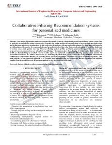
Figure 1: No. of NaNs (a)ML (b)YH (c)NF • HB1:
rˆui =
r¯ + u r¯ + u
PK s(U ,U )(rki −¯ rk ) k=1 PK u k k=1 |s(Uu ,Uk )| PN u rk ) k=1 s(Uu ,Uk )(rki −¯ PNu k=1 |s(Uu ,Uk )|
if Nu ≥ K +
PK−Nu s(Uu ,Uks )(IRk −¯ rk ) k=1 PK−Nu |s(Uu ,Uks )| k=1
if Nu < K (5)
• HB2: rˆui =
r¯u + r¯ + u
PK s(U ,U )(rki −¯ rk ) k=1 PK u k k=1 |s(Uu ,Uk )|
if rki 6= 0 (6)
PK
IR
s(U ,U )( rk ) k −¯ k=1 PK u k k=1 |s(Uu ,Uk )|
if rki = 0
where the similarity between the users are calculated by the Jaccard similarity in user-user network.
4
Experimental Evaluation
We conducted experiments on three real datasets, namely, Movielens (ML), Yahoo (YH) and Netflix (NF). Detailed description is given in Table 1. We utilized these datasets in two different ways to show the efficiency of our approaches on original dataset (Experiment 1 setup) as well as in sparse scenarios (Experiment 2 setup). We apply user-based method on Movielens and Netflix datasets and item-based method on Yahoo dataset as items are quite less compared to users in YH dataset.
4.1
Experiment 1 Setup
This setup is to show how the predictions differ for different users (items) based on the numbers of ratings a user made (an item received). We divided each dataset into 4 parts as described in (Table 2). 1. U20-25 ( I20-25): The U20-25 is a group of users who have rated number of items between 20-25. There are total 491 users in ML dataset.
8
Dataset M ovielens Y ahoo N etf lix
Ratings per user (item) 20-25 100-149 ≥150 ≥ 20 491 849 2096 6040 (3) (243) (518) (998) 6 551 1991 4139
Table 2: Division of datasets used in experiment 1 setup. Likewise, I20-25 is set of items which are rated by number of users between 20-25. There are only three (3) items in YH. So, this set consists of very sparse user (item) vectors. We see the effect of data sparsity on prediction for these users (items). Neighborhood selection is done from whole dataset. 2. U100-149 (I100-149): U100-149 is the set of users who have rated a significant number of items in ML and Netflix datasets. Similarily, I100149 is set of items which are rated by number of users between 100 and 149. There are such 243 items in YH. So, this set consists of users (items) which have significant ratings. 3. UGE150 (IGE150) : UGE150 is set of users who have rated more than 149 number of items. Similarily, IGE150 is set of items which are rated by more than 149 number of users. 4. UGE20 (IGE20): This set consists of user (item) vectors from whole dataset. To compare prediction performance for different category we randomly select 150 users (items) from each category. If total number of users (items) in a set is less than 150, we select all of them in that category. For each user, we randomly delete 15 ratings. Deleting more than 15 entries for test purpose will mostly result in void or very sparse vector(only 1 or 2 ratings). We predict these deleted ratings using state of art methods and methods proposed in this paper.
4.2
Experiment Setup 2
Main objective of the experiment setup 2 is to show the performance of our network based similarity measures on sparse datasets made from original datasets. We removed 75 % ratings from each user (item) to make them sparse dataset. It may be noted that during sparsing process all ratings of few items (users) are deleted fully. Description of these sparse datasets is given in Table 3. Dataset M ovielens Y ahoo N etf lix
Purpose Movie Music Movie
|U| 6040 15082 4141
|I| 3517 1000 8094
#Ratings(RT) 0.25 M 0.08M 0.25 M
|U|/|I| 1.71 15.08 0.51
κ=
RT ×100 |U |×|I|
Table 3: Description of the Sparse datasets used in the experiments.
9
1.18 0.51 0.69
NHSM
CN
1.15 1.1 1.05 0
50
100 K−Neighbors
150
1 0.95 0.9 0.85 0
Jaccard RMSE for U100−149
PIP
RMSE for UGE20
RMSE for UGE150
RMSE for U20−25
PCC 1.2
50
100 K−Neighbors
150
Katz
HB2
HB1
1.15 1.1 1.05 1 0.95 0
50
100 K−Neighbors
150
50
100 K−Neighbors
150
1.1 1.05 1 0
Figure 2: RMSE in Movilens PCC
PIP
NHSM
CN
MAE for UGE150
MAE for U100−149
0.95 0.9
0
50
100 K−Neighbors
150
0.8 0.75 0.7 0.65 0
Jaccard
50
100 K−Neighbors
HB2
HB1
0.9 0.85 0.8 50
100 K−Neighbors
150
50
100 K−Neighbors
150
0.9
0.85
0.8 0
150
Katz
0.95
0
MAE for UGE20
MAE for U20−25
1
Figure 3: MAE in Movilens
4.3
Metrics
We use various evaluation metrics to compare the accuracy of the results obtained by our network based CF and other neighborhood based CFs. Two popular quantitative metrics (Root Mean Squared Error and Mean Absolute Error) and one popular qualitative metric (F1 measure) are used. For the shake of readability, we discuss them briefly. Finally, we introduce a new qualitative measure termed as Best Common Rated Item (BCRI) to address the drawback of the F1 measue in recommendation scenario. 1. Root Mean Squared Error(RMSE): Let Xu =[eu1 , eu2 , eu3 ...eu1m ] be the error vector for m rating prediction of a user Uu . A smaller value indicates a better accuracy. Root Mean Square Error(RMSE) for a user 10
PCC
PIP
NHSM
CN
Jaccard
Katz
HB2
HB1
BCRI for U100−149
BCRI for U20−25
2.8 2.7 2.6 2.5 2.4 0
50
100 K−Neighbors
150
2.9 2.8 2.7 0
50
100 K−Neighbors
150
50
100 K−Neighbors
150
BCRI for UGE20
BCRI for UGE150
3 3 2.9 2.8 2.7 2.6 0
50
100 K−Neighbors
2.9 2.8 2.7 2.6 0
150
Figure 4: BCRI in Movilens is computed as follows. RM SE =
r Pm
2 i=1 eui
m
2. Mean Absolute Error(MAE): Mean Absolute Error measures average absolute error over m predictions for a user Uu . It is computed as follows. M AE =
Pm
|eui | m
i=1
3. F1 Measure: Many recommender systems provide a list of items Lr to an active user instead of predicting ratings. There are two popular metrics to evaluate quality of a RS in this scenario: (i)P recision, which is the fraction of items in Lr that are relevant and (ii)Recall, which is the fraction of total relevant items that are in the recommended list Lr . A list of relevant items Lrev to a user is the set of items on which she made high ratings (i.e, ≥ 4 in MovieLens dataset) in the test set. Therefore, P recision and Recall can be written as follow. P recision =
|Lr ∩Lrev | and |Lr |
Recall =
|Lr ∩Lrev | |Lrev |
However, there is always a trade-off between these two measures. For instance, increasing the number of items in Lr increases Recall but decreases P recision. Therefore, we use a measure which combines both called F 1 measure in our experiments. F1 =
2 × P recision × Recall P recision + Recall
4. Best Common Rated items: The F1 measure is very popular among information retrieval community. However, it is not suitable measure in the following scenario. There are users who are very lenient in giving ratings, e.g T om has given minimum rating value of 4 to items. On the 11
1.12 PCC
PIP
NHSM
CN
Jaccard
Katz
HB2
HB1
1.1 1.08
RMSE for ML
1.06 1.04 1.02 1 0.98 0.96 0
50
100
150
K−Neighbors
Figure 5: RMSE in Sparse ML 0.9 PCC
PIP
NHSM
CN
Jaccard
Katz
HB2
HB1
0.88 0.86
MAE for ML
0.84 0.82 0.8 0.78 0.76 0.74 0.72 0
50
100
150
K−Neighbors
Figure 6: MAE in Sparse ML other hand, there are users who are very strict on giving ratings, e.g Siddle has given at maximum rating value 2 to items. For strict users, it is difficult to find Lrev the set of items on which she made high ratings (i.e, ≥ 4 ) as such ratings are not present. Also if no predicted rating is ≥ 4, we can not compute Lr . To measure performances in such scenario, we introduce a new metric termed as Best Common Rated Items (BCRI). It determines whether best actual rated entries are also best predicted entries or not. Let BAI = {ba1 , ba2 , ba3 , ba4 , ba5 } be the set of top t best rated items by a user and BP I be the set of top t best predicted items for the user. BCR is computed as follows. BCRI = BAI ∩ BP I
12
0.9 PCC
PIP
NHSM
CN
Jaccard
Katz
HB2
HB1
0.85 0.8
F1 for ML
0.75 0.7 0.65 0.6 0.55 0.5 0.45 0
50
100
150
K−Neighbors
Figure 7: F1 in Sparse ML
4.4
Experimental Results and Analysis
In experiment setup 1, from each subset we selected users or items and predicted deleted ratings using all other users or items in the corresponding rating dataset. As we know traditional similarity measures use ratings of only co-rated items in case of user-based CF, whereas, they use ratings of common users in case of item-based CF. Therefore, in many situation we cannot find similarity between a pair of users (items). This is reflected in figure1. In figure 1, we get many times NaNs during similarity computations specifically while computing similarity for users in the first group U20-25. It can be noted that if similarity come out to be NaN, we can not use it for prediction purpose. This shows that sparsity is a big issue in computing similarity using traditional similarity measures. For Yahoo dataset we use item-based method as number of items is quite less than number of users. In this dataset, when we select items from IGE20 for computing similarity, we find many NaNs (8460) for 150 items. Similar trends are found for other groups of items. Similarly in Netflix data set, When we select users from UGE20 total number of NaNs during similarity calculation for 150 users is 35816 and when we select users from U20-25 it is 14535(for 6 users), where as for U100-149 , UGE150, the numbers are significantly less, i.e 12881, 2932 respectively . So we can see that few co-rated entries are hindrance in determining similarities between a pair of user or items. We use structural similarity measures to get rid of this problem. We begin analyzing results of the experiments with Movielens dataset. Results of experiment setup 1 on Movielens is shown in Figure 2- 4. In general RMSE, MAE decrease, while BCRI increases with increase of nearest neighbors. The state-of-the-art similarity measure NHSM performs better than PIP in RMSE (Figure 2), MAE (Figure 3), BCRI. However, for large value of K PIP outperforms NHSM and other traditional measures in RMSE, MAE. From Figure 2- 4, it is found that structural similarities based CFs outperforms PCC measure based as well as state of art similarities based CFs in each metric. Hybrid methods outperforms all other similarity measures in RSME, MAE. However, for small value of K Jaccard similarity obtained from network outperforms hybrid methods in BCRI. The HB1 is best. Among different categories, pre13
PIP
NHSM
CN
Jaccard RMSE for I100−149
1.3 1.25 1.2 1.15 0
50
100 K−Neighbors
150
HB2
HB1
1.2
1.1 50
100 K−Neighbors
150
50
100 K−Neighbors
150
1.25
1.15 1.1 1.05 1 0.95 0
Katz
1.3
0
RSME for IGE20
RMSE for IGE150
RMSE for I20−25
PCC 1.35
50
100 K−Neighbors
1.2 1.15 1.1 0
150
Figure 8: RMSE in Yahoo diction performance for users in UGE150 is best while for users in UB20-25 is worst, it clearly shows that performance is relatively good for dense vectors. Results of experiment setup 2 on sparse Movielens subset are shown in figure 5-7. In figure 5, it can be noted that traditional similarity measure PCC performs poorly badly compared to the state of the art similarity measures. Recently proposed NHSM outperforms PIP measures in RMSE. However, all structural similarities computed from proposed network of users outperform PIP, NHSM and PCC measures in RMSE. Hybrid techniques are found to be outperforming other structural similarly measures derived from the network. In Figure 6, MAE of the CFs are plotted over increasing value of K. Similar trends are noted here also. Structural similarly measures based CFs outperform PCC and NHSM and PIP measures. Two hybrid techniques which are proposed to remove K-neighbor problem is found to be better than other structural similarity measures. The first hybrid approach makes least MAE as low as 0.82 at the value of K = 150. The plot in figure 7 shows the efficiency of our structural similarity (extracted from network) based CFs over others measures based CFs. The F1 measure is used to show the capability of an approach to retrieve relevant items in a user’s recommended list. It is found that hybrid approach including other structural similarly outperform PCC, PIP and NHSM measures in F1 measures. This facts justifies our claim that hybrid approaches with network can address the problem of data sparsity. It can be noted that sparsity of the ML subset is 98.82% (Table 3).
Results of experiment setup 1 on Yahoo dataset is shown in figure 8- 10. In general RMSE, MAE decreases, while BCRI increases with K-N eighbors. NHSM performs better than PIP in RMSE, MAE, BCRI but for large value of K, PIP performs better in RMSE, MAE than NHSM. It is observed that
14
PCC
PIP
NHSM
CN
Jaccard 1.1 MAE for I100−149
MAE for I20−25
1.15 1.1 1.05 1 0
50
100 K−Neighbors
HB1
1 0.95 0.9 0
50
100 K−Neighbors
150
50
100 K−Neighbors
150
1.05 MAE for IGE20
MAE for IGE150
HB2
1.05
150
0.95 0.9 0.85 0.8 0.75 0
Katz
50
100 K−Neighbors
1 0.95 0.9 0
150
Figure 9: MAE in Yahoo
CN
2.4
50
100 K−Neighbors
150
2.7 2.6 2.5
Katz
HB2
HB1
2.7 2.6 2.5 0
2.8
2.4 0
Jaccard BCRI for I100−149
NHSM
2.5
2.3 0
BCRI for IGE150
PIP
BCRI for IGE20
BCRI for I20−25
PCC
50
100 K−Neighbors
150
50
100 K−Neighbors
150
2.7 2.6 2.5 2.4
50
100 K−Neighbors
150
0
Figure 10: BCRI in Yahoo
15
1.24
PCC
PIP
NHSM
CN
Jaccard
Katz
HB2
HB1
1.22
RMSE for YH
1.2 1.18 1.16 1.14 1.12 1.1 1.08 0
50
100
150
K−Neighbors
Figure 11: RMSE in Sparse YH 1.04 PCC
PIP
NHSM
CN
Jaccard
Katz
HB2
HB1
1.02 1
MAE for YH
0.98 0.96 0.94 0.92 0.9 0.88 0
50
100
150
K−Neighbors
Figure 12: MAE in Sparse YH structural similarities outperforms PCC and state of art similarities in RMSE, MAE. Hybrid methods along with other structural measures outperform PIP, NHSM, PCC similarity measures in RMSE, MAE and BCRI metrics. Among the proposed measures, HB1 is best in all metrics. It can be noted that we applied item-based CF on Yahoo dataset.
To show the efficiency of the proposed network approach, we compare the performance of item-based CFs on Yahoo dataset and results are reported in figure 11- 13. In Figure 11 and Figure 12, predictive metrics RMSE and MAE of different similarity measures based CFs are plotted over the value of K. In the both plots, it is found that structural similarity obtained from item network can provide better RMSE and MAE values compared to PCC, PIP and recently 16
0.8
PCC
PIP
NHSM
CN
Jaccard
Katz
HB2
HB1
0.75 0.7
F1 for YH
0.65 0.6 0.55 0.5 0.45 0.4 0
50
100
150
K−Neighbors
Figure 13: F1 in Sparse YH PIP
NHSM
CN RMSE for U100−149
RMSE for U20−25
PCC 1.25 1.2 1.15 1.1 1.05 0
50
100 K−Neighbors
150
RMSE for UGE20
RMSE for UGE150
0.95 0.9 0.85 0
50
100 K−Neighbors
150
Katz
HB2
HB1
1.1
1 0
1.05 1
Jaccard 1.2
50
100 K−Neighbors
150
50
100 K−Neighbors
150
1.15 1.1 1.05 1 0
Figure 14: RMSE in Netflix introduced NHSM measure. In figure 13, F1 measures of different structural similarity based CFs, PCC based CF and PIP and NHSM based CFs are shown in increasing value of K. PCC based CF is worst performer in F1 measure. The PIP measure based CF outperforms NHSM measure. All similarity extracted from item-item network are found to be outperforming traditional PCC, PIP and recently introduced NHSM measure. The hybrid techniques are found to be suitable in this highly sparse dataset. It can be noted that network approach is equally successful in item-based CF.
17
PIP
NHSM
CN
1 0.95 0.9 0
Jaccard 1 MAE for U100−149
MAE for U20−25
PCC
50
100 K−Neighbors
Katz
HB2
HB1
0.95 0.9 0.85 0.8
150
0
50
100 K−Neighbors
150
50
100 K−Neighbors
150
MAE for UGE20
MAE for UGE150
0.85 0.8 0.75 0.7 0.65 0
50
100 K−Neighbors
0.9 0.85 0.8 0
150
Figure 15: MAE in Netflix
CN
2.2 2 50
100 K−Neighbors
Katz
HB2
HB1
2.7 2.6 2.5 0
150
50
100 K−Neighbors
150
50
100 K−Neighbors
150
2.8
2.9 2.8 2.7 2.6 2.5 0
Jaccard 2.8 BCRI for U100−149
NHSM
2.4
0
BCRI for UGE150
PIP
BCRI for UGE20
BCRI for U20−25
PCC 2.6
50
100 K−Neighbors
2.7 2.6 2.5
150
0
Figure 16: BCRI in Netflix
1.22 PCC
PIP
NHSM
CN
Jaccard
Katz
HB2
HB1
1.2
RMSE for NF
1.18 1.16 1.14 1.12 1.1 1.08 1.06 0
50
100 K−Neighbors
Figure 17: RMSE in Sparse NF
18
150
1
PCC
PIP
NHSM
CN
Jaccard
Katz
HB2
HB1
0.98
MAE for NF
0.96 0.94 0.92 0.9 0.88 0.86 0.84 0
50
100
150
K−Neighbors
Figure 18: MAE in Sparse NF
0.8
PCC
PIP
NHSM
CN
Jaccard
Katz
HB2
HB1
0.75
F1 for YH
0.7 0.65 0.6 0.55 0.5 0.45 0.4 0
50
100 K−Neighbors
Figure 19: F1 in Sparse NF
19
150
Results of experiment setup 1 on Netflix is shown in figure 14- 16. NHSM performs better than PIP for smaller values of K in RMSE, MAE, BCRI metrics. However, PIP outperforms NHSM in large value of K. We see that structural similarities outperform PCC and state of art similarities in RMSE, MAE and BCRI measures. Hybrid methods outperforms all other similarity measures in RSME, MAE and BCRI metrics. The HB1 is best in all metrics. Experimental results of experiment setup 2 on sparse Netflix dataset is shown in figure 17- 19. Simialr trends are noted. Structural similarities based CF outperform PCC, PIP and NHSM based CFs in MAE, RMSE and F1 measure on highly sparse Netflix subset. For smaller value of K, NHSM performs better than CN. However, with suitable number of nearest neighbors, hybrid methods perform better than other similarity measures in RMSE, MAE and F 1 metrics. The HB1 is the best in all metrics even on sparse datasets.
5
Conclusion
In this work, we proposed a new outlook to deal with the problem of collaborative recommendation by gainfully using the concept of structural similarity of nodes in a complex network after generating user-user and item-item networks based on the given data. We showed that, the curse of sparsity and K-neighbors problem can be delicately handled in this approach. Thus, we proposed CFs based on structural similarity measures of the user-user and itemitem networks individually. Moreover, we introduced two methods which we call hybrid methods using both user-user and item-item networks for CF . We verified the effectiveness of these measures by comparing its performances with that of neighborhood based CFs using state-of-the-art similarity measures when applied to a set of real data. The comparison results established that the proposed measures based CFs and hybrid methods outperform existing similarity measures based CFs in various evaluation metrics.
References [1] Kamal Ali and Wijnand Van Stam. Tivo: making show recommendations using a distributed collaborative filtering architecture. In Proceedings of the tenth ACM SIGKDD international conference on Knowledge discovery and data mining, pages 394–401. ACM, 2004. [2] Daniel Billsus, Clifford A Brunk, Craig Evans, Brian Gladish, and Michael Pazzani. Adaptive interfaces for ubiquitous web access. Communications of the ACM, 45(5):34–38, 2002. [3] Keunho Choi and Yongmoo Suh. A new similarity function for selecting neighbors for each target item in collaborative filtering. Knowledge-Based Systems, 37:146–153, 2013. [4] Luis M De Campos, Juan M Fern´ andez-Luna, Juan F Huete, and Miguel A Rueda-Morales. Combining content-based and collaborative recommendations: A hybrid approach based on bayesian networks. International Journal of Approximate Reasoning, 51(7):785–799, 2010.
20
[5] Christian Desrosiers and George Karypis. A comprehensive survey of neighborhood-based recommendation methods. In Recommender systems handbook, pages 107–144. Springer, 2011. [6] Michael D Ekstrand, John T Riedl, and Joseph A Konstan. Collaborative filtering recommender systems. Foundations and Trends in HumanComputer Interaction, 4(2):81–173, 2011. [7] Michael D Ekstrand, John T Riedl, and Joseph A Konstan. Collaborative filtering recommender systems. Foundations and Trends in HumanComputer Interaction, 4(2):81–173, 2011. [8] Thomas Hofmann. Latent semantic models for collaborative filtering. ACM Transactions on Information Systems (TOIS), 22(1):89–115, 2004. [9] Dietmar Jannach, Markus Zanker, Alexander Felfernig, and Gerhard Friedrich. Recommender systems: an introduction. Cambridge University Press, 2010. [10] Dietmar Jannach, Markus Zanker, Alexander Felfernig, and Gerhard Friedrich. Recommender systems: an introduction. Cambridge University Press, 2010. [11] Joseph A Konstan and John Riedl. Recommender systems: from algorithms to user experience. User Modeling and User-Adapted Interaction, 22(12):101–123, 2012. [12] Yehuda Koren. Factorization meets the neighborhood: a multifaceted collaborative filtering model. In Proceedings of the 14th ACM SIGKDD international conference on Knowledge discovery and data mining, pages 426– 434. ACM, 2008. [13] Ken Lang. Newsweeder: Learning to filter netnews. In Proceedings of the 12th international conference on machine learning, pages 331–339, 1995. [14] Greg Linden, Brent Smith, and Jeremy York. Amazon. com recommendations: Item-to-item collaborative filtering. Internet Computing, IEEE, 7(1):76–80, 2003. [15] Haifeng Liu, Zheng Hu, Ahmad Mian, Hui Tian, and Xuzhen Zhu. A new user similarity model to improve the accuracy of collaborative filtering. Knowledge-Based Systems, 56:156–166, 2014. [16] Linyuan L¨ u and Tao Zhou. Link prediction in complex networks: A survey. Physica A: Statistical Mechanics and its Applications, 390(6):1150–1170, 2011. [17] Michael Pazzani and Daniel Billsus. Learning and revising user profiles: The identification of interesting web sites. Machine learning, 27(3):313– 331, 1997. [18] Michael J Pazzani and Daniel Billsus. Content-based recommendation systems. In The adaptive web, pages 325–341. Springer, 2007.
21
[19] Paul Resnick, Neophytos Iacovou, Mitesh Suchak, Peter Bergstrom, and John Riedl. Grouplens: an open architecture for collaborative filtering of netnews. In Proceedings of the 1994 ACM conference on Computer supported cooperative work, pages 175–186. ACM, 1994. [20] Paul Resnick and Hal R Varian. Recommender systems. Communications of the ACM, 40(3):56–58, 1997. [21] Xiaoyuan Su and Taghi M Khoshgoftaar. A survey of collaborative filtering techniques. Advances in artificial intelligence, 2009:4, 2009. [22] Koen Verstrepen and Bart Goethals. Unifying nearest neighbors collaborative filtering. In Proceedings of the 8th ACM Conference on Recommender systems, pages 177–184. ACM, 2014.
22