A complex network-based approach for boundary shape analysis Andr´e Ricardo Backes Universidade de S˜ ao Paulo Instituto de Ciˆencias Matem´ aticas e de Computa¸c˜ ao
[email protected]
Dalcimar Casanova Universidade de S˜ ao Paulo Instituto de Ciˆencias Matem´ aticas e de Computa¸c˜ ao
[email protected]
Odemir Martinez Bruno Universidade de S˜ ao Paulo Instituto de Ciˆencias Matem´ aticas e de Computa¸c˜ ao
[email protected]
Abstract This paper introduces a novel methodology to shape boundary characterization, where a shape is modeled into a Small World complex network. It uses degree and joint degree measurements in a dynamic evolution network to compose a set of shape descriptors. The proposed shape characterization method has an efficient power of shape characterization, it is robust, noise tolerant, scale invariant and rotation invariant. of A leaf plant Classification experiment is presented on three image databases in order to evaluate the method and compare it with other descriptors in the literature (Fourier descriptors, Curvature, Zernike moments and Multiscale Fractal Dimension). Key words: Shape Analysis, Shape Recognition, Complex Network, Small-World Model
1
Introduction
In pattern recognition and image analysis, shape is one of the most important visual attributes to characterize objects. It provides the most relevant
Preprint submitted to Elsevier
31 May 2008
information about an object in order to identify and classify tasks [1, 2]. In recent years, significant progress has been made in research over shape signatures and recognition [3, 2, 4]. According to Pavlids [5], there are mainly two approaches to shape representation, namely, (1) the region-based approach, that use moment descriptors to describe shapes [6, 7, 8] and (2) the boundarybased approach que tend to be more efficient for handling shapes that are describable by their object contours [9]. This class of techniques include, among others, Fourier descriptors [10, 11, 12], Curvature Scale Space (CSS) [9, 13], wavelet descriptors [14] and Multiscale Fractal Dimension [2, 15]. There are a very large number of shape signatures schemes in the literature, good surveys can be found in [16, 17, 5]. This work is related to the approach two, shape boundary-based approach. The literature presents various methods to analyze images and objects using shape boundary, and the basis of most of them considers the shape as a chain of connected points [1]. In this approach, the sequence of the points in the boundary perform an important role, as it is used to extract the shape signature or descriptor that is capable of characterizing the shape boundary. The method proposed here, has a novel approach to the shape boundary analysis using the Complex Networks Theory [18, 19, 20, 21]. It considers the shape boundary as a set of points and models this set as a graph. The topology of an Small World network model is obtained artificially by transformations on vertices of shape model. The topological features, derived from the dynamics of the network growth, are correlated to physical aspects of the shape. Consequently, these measurements can be used to compose a shape descriptor or signature. These descriptors may be used to identify and distinguish objects. Traditional shape boundary methods yield the shape descriptors using the contour as continuous closed curves formed by the adjacent sequential pixels. By modeling the shape boundary as complex network, the method proposed here, on the other hand, does not need adjacent and sequential pixels as the graph model only takes the distance between the boundary elements into account. As will be shown in this paper, the proposed method presents better results in shape characterization. Besides, due to the graph approach, it is more robust as it does not need sequential closed continuous curves of contours. Thus, it can characterize degraded boundary shapes, that have incomplete information such as gaps or holes. It is also noise tolerant and is invariant to scale and rotation. In order to evaluate the proposed method, a set of shape characterization experiments was done. The main aim of the experiments is to perform plant species classification using the leaf shape boundary. In the experiment, the 2
leaves were intentionally re-shaped in order to evaluate characteristics such as noise tolerance, robustness, scale invariance and rotate invariance. We also did the experiment with other descriptors found in the literature to compare the results and features with the novel method. Additionally, more two tradicional shape databases are used to corroborate the efficiency of this novel method. The data from the experiments were evaluated by the use of the linear discriminant analysis (LDA) [22]. The LDA also enable us to verify the distribution of clusters in the feature space. A descriptor is considered ”good” when it creates compact clusters far away from each other for all classes in the corresponding feature space. This paper starts by presenting an overview of the Complex Network Theory (Section 2). In Section 3, the method is detailed. The following is presented: how to model the shape as a complex network and by using Complex Network Theory to extract different network measures which are related with the object shape. These network measures are used to compose the shape descriptors that characterize the shape of an object. Section 4 presents the results of experiments using the three image databases of shapes contours, where the novel method was compared with other shape descriptors and various aspects are discussed (shape characterization power, rotation invariance, scale invariance, noise tolerance, robustness and the capability to deal with degraded contours). We present the conclusion and our current research on shape descriptors in Section 5.
2
Complex Networks
Complex networks research can be described as the intersection between graph theory and statistical mechanics, which confers a truly multidisciplinary nature to this area, since it integrates computer sciences, mathematics and physics [20]. Due to its great flexibility and generality, the current interest has focused on applying the developed concepts to many real data and situations. Although many topics of computer vision can be modeled using these concepts, this still is a unexplored field, and only few references are found in literature [23]. The existent studies include investigations of the problem representation as a Complex Network, followed by an analysis of dynamics of the network growth and topological characteristics. In [24] and [25] are presented the use of complex networks for modeling texts and image textures. These works model the problem as an complex network and use traditional measurements of the network connectivity to obtain feature 3
vectors from which the texts and textures images can be characterized and classified. The main idea of this work is to represent a shape in terms of a Watts-Strogatz network model [26] followed by analyzing of its topological and dynamics characteristics. This network model presents what is called the small world property, i.e., all vertices can be reached from any other through a small number of edges, and also present a large number of loops of size three, i.e., if vertex i is connected to vertices j and k, there is a high probability of vertices j and k being connected (the high clustering coefficient). The model is situated between an ordered finite lattice and a random graph. The dynamic model of Small World network is obtained artificially by sequential thresholds on vertices of shape model. We show that shape format is correlated with Small-World network structure on many stages of network growth. The study of its dynamical proprieties (metrics was derived from the dynamics of the network growth, based on the variation of the number of connected components) produce a shape signature, so this signature can be used for image analysis and classification processes. This process is described in following sections.
2.1
Measurements on Complex Networks
Each complex network presents specific topological features which characterize its connectivity and highly influence the dynamics and function of processes executed in the network. The analysis and discrimination of a complex network therefore rely on the use of measurements capable of expressing the most relevant topological features and their subsequent classification. Below, the measurements used in this work are presented. A complete survey of measurements can be seen in [20].
2.1.1
Degree
The degree (or connectivity) ki of a node i is the number of edges directly connected to node, and it is defined in terms of the adjacency matrix A as: ki =
N X
aij ,
j=1
where N is the number of vertices in the network. The degree is an important characteristic of a vertex. Based on the degree of the vertices, measures can be extracted from the network. Two of the simplest 4
measures are the maximum degree: kκ = max ki i
and average degree kµ =
2.1.2
N 1 X ki . N i=1
Joint Degree
Another interesting possibility is to find a correlation between the degrees of different vertices. Correlations play an important role in many structural and dynamic network properties [27]. The most common choice is to find correlations between two vertices connected by an edge. This correlation can be expressed by the joint degree distribution P (ki , k 0 )i , i.e., the probability of existing an edge connecting the vertex i, with degree ki , to another vertex of the network, with degree k 0 . The choice of k 0 can be performed of an arbitrary way, and for this case we considered ki = k 0 . In other words, P (ki , k 0 )i shows the probability of a vertex i having a neighbor with the same degree. There are various measures that can be extracted by analyzing this probability distribution, such as entropy, energy and the average joint degree. Entropy, historically, has often been associated with the amount of order, disorder, and/or chaos in a system [28]. It is defined as: H=−
N X
P (ki , k 0 )i log2 P (ki , k 0 )i
i=1
The energy of a system is: E=
N X
(P (ki , k 0 )i )2
i=1
The average joint degree denotes the probability of finding two arbitrary nodes in the network with the same degree: N 1 X P (ki , k 0 )i . P = N i=1
5
2.2
Dynamic evolution
Another important characteristic in complex networks is its evolution dynamic, which affects various network properties [20, 18]. As an immediate consequence, the measurements of the complex networks are a function of time, i.e., two networks achieved at distinct instants from the same underlying dynamics are characterized by different features. Although, we often only have access to a given configuration obtained from an unknown dynamic evolution, sometimes a series of samples throughout an evolution of this kind is available. This is a typical system which can be monitored over time. In these cases, it becomes particularly interesting to consider the trajectories of some measures (and not only isolated points in the feature space) as a way to analyze and classify networks. This provides a more comprehensive characterization of the network under analysis. In addition, considering measurements as a function of time, it would also be interesting to try to characterize classes of complex networks by considering the dynamics of the respectively defined feature space [20].
3
Complex Network Shape Signature
In this section, the following is proposed: how to model the shape boundary as a Complex Network and afterwards extract two distinct feature vectors which are the Degree Descriptors and the Joint Degree Descriptors showing how to use the tools from the Complex Networks Theory to create a feature vector to discriminate a contour shape.
3.1
Complex Network Model
Consider S as the contour of an image, where S = [s1 , s2 , ..., sN ] and si , are typical vectors in the form of si = [xi , yi ], whose components are discrete numerical values representing the coordinates of point i of the contour. In order to apply the Complex Networks Theory to the problem, a representation of contour S should be built like graph G = hV, Ei. Each pixel of the contour is represented as a vertex in the network (i.e., S = V ). A set of non-directed edges E binding each pair of vertices makes up the network. This set E is calculated using the Euclidean distance:
d(si , sj ) =
q
(xi − xj )2 + (yi − yj )2 . 6
Therefore, the network is represented by the N × N weight matrix W ,
wij = W ([wi , wj ]) = d(si , sj ), normalized into the interval [0, 1],
W =
W . maxwij ∈W
Initially, the set of edges E connects all network vertices to each other. This means that the network behaves regularly, once all their vertices have the same number of connections. However, a regular network is not considered a complex network, not presenting any relevant property for the developed application. Thus, it is necessary to transform this regular network into a complex network that owns relevant properties for the application.
Fig. 1. Representation of contour modeled as a Complex Network
A possible way of carrying out this transformation is to apply a threshold Tl which produces a new set of edges for the network. This transformation is performed by selecting the group of edges Eb of E, so that the selected edges have smaller weight than parameter Tl . This approach allows to convert a network initially regular in a complex network that fits in the Small-World model proposed by Watts and Strongatz [26]. This complex network model is characterized by two basic properties: (i) high clustering coefficient and (ii) the 7
small-world property. Clustering coefficient is a measure of how interconnected network vertices are, and it is defined as C = 3N∆ /N3 , where N∆ is the number of existing triangles in the network and N3 the number of connected triples. A connected triple occurs when a vertex i is connected to a vertex j, and j is connected to vertex k. A triangle occurs when vertices i and k are also connected. The small-world property is a consequence of a high clustering coefficient, once the more the vertices are interconnected, the more paths between a pair of vertices are possible. This property is characterized by the existence of a small average geodesic path in the network, where a geodesic path is the shortest path in the network connecting two vertices i and j, where i 6= j. The example of a contour modeled as a Complex Network can be seen in Figure 1. For this representation, coordinates x and y are the same as in the original contour and coordinate z is the degree of the node. Figure 2 shows that the modeled network presents both high clustering coefficient and smallworld property (characterized by small average geodesic path), regardless of the threshold value used. Once the shape contour is modeled as a complex network, some of its properties can be quantified. This task, which consists of one of the basic steps in pattern recognition is performed as described in the following sections.
(a)
(b)
Fig. 2. Properties computed from a shape modeled as a Small World Complex Network (N = 353): (a) Average Geodesic Path Length; (b) Clustering Coefficient.
3.2
Dynamic evolution signature
The use of concepts and tools underlying complex network research can provide relevant information for image and object characterization. In light of 8
this, the idea proposed by this work is: given a specific transformed shape representation presented in the previous section, the respective characterization of shape S can be made by a feature vector obtained from different values of Tl from a δ transformation. This operation, henceforth represented as A = δTl (W ), is applied to each element of weighed matrix W , yielding the unweighed matrix A. Thus:
ATl = δTl (W ) = ∀w ∈ W
aij
= 0, if wij ≥ Tl
a
= 1, if wij < Tl
ij
In other words, the characterization is performed using various transformations δ where threshold Tl is incremented at a regular interval Tinc . Therefore, given set T , an element Tl ∈ T is defined by function f : T → T , where: T0 = Tini |0 < Tini < 1 Tl+1 = f (Tl ) if Tl < TQ < 1 f (x) = x + Tinc with Tini and TQ , respectively, the initial and final thresholds are defined by the user. This approach makes a signature which describes the temporary characteristics of the network dynamic evolution as shown in Figure 3.
(a)
(b)
(c)
Fig. 3. Network dynamic evolution by a threshold Tl and zoom area: (a) Tl = 0.1; (b) Tl = 0.15 and (c) Tl = 0.2.
Given some networks obtained for the dynamic evolution, the use of two distinct feature vectors are proposed for the characterization of shape S, the 9
Degree Descriptors and the Joint Degree Descriptors.
3.2.1
Degree descriptor
Degree descriptors are calculated from the transformed matrix A for each instant Tl using the average degree (kµ ) and max degree (kκ ) measurements, presented in Section 2.1.1. However, a normalization of the vertices degree by the number of vertices in the network is necessary before computing these measurements. This normalization is performed in order to reduce the influence of the network size in the computed descriptors, and it is performed as follows: ki ∀ki = . N Considering the network transformation at each instant time Tl , vector ϕ is computed as the concatenation of the average degree (kµ ) and max degree (kκ ) computed at each stage of the network evolution:
ϕ = [kµ (T0 ), kκ (T0 ), kµ (T1 ), kκ (T1 ), . . . , kµ (TQ ), kκ (TQ )] . Fig. 4 shows the process of computing the degree descriptors from an image. The presented feature vector, ϕ, can be used as a feasible shape signature which presents desirable properties for shape analysis, such as, scale and rotation invariance, noise tolerance and robustness: • Rotation and Scale invariance: The normalization of matrix W at interval [0, 1] ensures important properties of scale and the rotation invariance: Considering images at different scales, the normalization of W for maxwij fix the largest network edge (higher Euclidean distance between any 2 nodes) with a weight equal to 1, the same way the remaining edges are also normalized acquiring relative weights from the network size. This property can better be understood by observing Figure 5. Considering images in different rotations, the largest edges are preserved, regardless of the direction where it is found, thus, the normalization ensures the same properties for the set of edge E. It only has only a small addition of error deriving from the calculation of the Euclidean distance. Figure 6 represents this property. In order to keep the scale invariance characteristic it is necessary to address the fact that images of different scales possess a different number of points composing its contour. Since S = V , as shown in 3.1, two similar contours SA = [sA1 , sA2 , ..., sAN ] and SB = [sB1 , sB2 , ..., sBM ], with (N 6= M ), produce different networks (GA 6= GB ), i.e., networks with different number of vertices. Thus, the calculation of ki is directly affected by the number of nodes N since this was fulfilled directly over its sum as shown in Section 2.1.1. The solution is to normalize degree ki to the size of the modeled 10
Fig. 4. Process of extraction of degree descriptor from an image
Fig. 5. Representation of scale invariance property
network as presented previously 3.1. The possible physical interpretation is that the new ki contains the degrees normalized by the size of the modeled network (i.e. relative degrees of size network). Figure 7 demonstrates this transformation carried out by each ki . Figure 7a shows the degree of all network nodes, ki , and the respective average degree, kµ , of the same sample at different scales. Figure 7b shows that the average degree of the two networks draw closer when the normalization of degrees for the network size is carried out, i.e., although the curves 11
Fig. 6. Representation of rotate invariance property
(a)
(b)
Fig. 7. The effect of W normalization by network size: (a) before normalization; (b) after normalization.
possess a different number of nodes, the average and maximum degrees are equivalent. • Noise tolerance: During the shape digitalization step, small errors and variations can appear in the contour. These errors are justified because the acquisition process is a non-perfect task, and it is submitted to various kinds of interference and/or noise. The way that the shape contour is modeled as a complex network allows it to deal with different levels of noise, avoiding misclassification errors. • Robustness: The network model does not have space and sequential information of the modeled shape, which theoretically makes all the modeled patterns equal when they are analyzed in the feature space. This property denotes (for this shape analysis application), that a sequential extraction of a contour for network modeling and feature extraction is not necessary. Only a list of the coordinates of the points that makes up the contour is needed. 12
3.2.2
Joint degree descriptor
Joint degree descriptors are calculated from the transformed matrix A for each instant Tl using the entropy (H), energy (E) and average joint degree (P ) measurements, as presented in Section 2.1.2. Considering the network transformation at each instant time Tl , vector ϑ is computed as the concatenation of the entropy, energy and average joint degree computed at each stage of the network evolution:
ϑ = [H(T0 ), E(T0 ), P (T0 ), . . . , H(TQ ), E(TQ ), P (TQ )] . Characteristics presented in degree descriptors, such as, scale and rotation invariance, noise tolerance and robustness, are also present in joint degree descriptors. However, as the joint degree concerns a probability distribution, the calculation of P (ki , k 0 )i is not related with the number of vertices in the network, N . Thus, normalization of vertex degrees is irrelevant, provided that entropy, energy and average joint degree measurements are calculated using probability values P (ki , k 0 )i where ki = k 0 .
4
4.1
Evaluation
Linear Discriminant Analysis
In order to analyze the features extracted from the boundary shapes, a statistical analysis was carried out. This analysis was done applying a Linear Discriminant Analysis (LDA) to the data. LDA is a well known method to estimate a linear subspace with good discriminative properties. The idea of this method is to find a projection of the data where the variance between the classes is large compared to the variance within the classes. As it is a supervised method, LDA needs class definitions for the estimation process [22, 29].
4.2
Experiments
To evaluate the performance of the proposed Degree and Joint Degree descriptors, experiments were conducted based on the classification of three image databases: (i) generic artificial shapes with variations in structure, (ii) fish contours and (iii) plant leaves shapes. The first image set is composed by 13
Fig. 8. Examples of generic shapes used in the experiments.
Fig. 9. Examples of variations in the generic shapes used in the experiments.
Fig. 10. Examples of fish images used in the experiments.
different shapes categories, where each category is composed by several variations in the shape structure. The fish contours database objectives to show the performance of the method on large databases composed by shapes under rotation and scale transformations. Leaves classification is a difficult task, as the between-class similarity is considerable while the within-class similarity is not suitable. Besides, overlaps can occur between adjacent parts of leaves. As a result, there can be major differences among boundary contours of leaves in the same category. The generic shapes is composed of 99 shapes previously classified into 9 categories of 11 images each (Fig. 8) [4, 30]. Each category allows variations in structure, as well as for occlusion, articulation and missing parts (Fig. 9). 14
Fig. 11. Some of the leaves images used in the experiments
Fig. 12. Examples of variation within a class.
The fish contours database is composed of 10 different manifestations (5 rotations and 5 scales) of each one of the 1100 fish contours obtained from the database available at [31]. So, the database is composed of 11000 contours grouped into 1100 classes of 10 samples each. Fig. 10 shows some examples of fish contours present in the database. The leaves database consists of 30 classes with 20 samples each. Fig. 11 shows the various classes used in the experiment, while Fig. 12 shows an example of variation within a class. In addition, to evaluate properties such as scale and rotation invariance, noise tolerance and robustness of the method, other 15
experiments were carried out with modified databases. The modifications are: (1) Rotation: The original database was rotated by the following angles: 7o , 35o , 132o , 201o and 298o . Therefore, the problem consists of 30 classes with 120 shapes each. Fig. 13 shows an example of the applied rotations.
Fig. 13. Examples of applied rotations
(2) Scale: Each image of the original database was scaled by the following factors: 200%, 175%, 150% and 125%. Therefore, the problem consists of 30 classes with 80 shapes each. An example of applied transformation can be seen in Fig. 14.
Fig. 14. Examples of applied scales
(3) Noise: In order to evaluate noise tolerance, four different levels of noise were added to the original database. The noise is uniformly generated at the interval [−n . . . n], where n is the intensity level of the noise and added to the original signal (Fig. 15). For shape contours, the noise pattern is generated for both x and y coordinates of the contour. The problem now consists of classifying 30 classes with 80 shapes each. An example of applied noise can be seen in Fig. 16. (4) Robustness in continuous degradation: Feature vector is expected to be able to classify a shape, even if this shape presents a lack in its contour. To verify this property 13 degradation levels (5%, 10%...65%) were applied to each sample of the original database. The aim of this is to observe the robustness of the proposed method against shape degradation. In this first experiment, the degradation is performed in a continuous way, i.e., only a part of the contour is lacking, and its sequential extraction is still possible. Fig. 17 shows an example of the continuos degradation of a contour. An experiment is done for each degradation level, and 30 classes with 20 samples each are considered. (5) Robustness in random degradation: Similar to the previous experiment, this one also uses 13 degradation levels (5%, 10%...65%), but this degradation is applied randomly to the original contour. For this reason, it is 16
Fig. 15. Example of noise generation: (a) Original signal; (b) Noise at Level 1; (c) Noisy signal.
Fig. 16. Examples of applied noises
Fig. 17. Examples of applied continuous degradation
not possible to extract the shape contour in a sequential way. Fig. 18 shows an example of the random degradation of a contour. An experiment is done for each degradation level, and 30 classes with 20 samples each are considered. In all experiments, the adjacency matrix A(Tl ) is obtained using the δ function, as described in Section 3.2, with an initial threshold Tini = 0.025, incremented at a regular interval of 0.075 until reaching a final threshold TQ = 0.95. As 17
Fig. 18. Examples of applied random degradation
presented in Sections 3.2.1 and 3.2.2, the average and maximum degree as well as the entropy, energy and average of the joint degree are calculated using the modeled network at each different threshold, making a total of 2 signatures (degree and joint degree) with 26 and 39 descriptors, respectively. The evaluation is made using statistical analysis in the descriptors using the LDA in a leave-one-out cross-validation scheme. We also compared the results achieved with other shape descriptors found in the literature using the same statistical analysis. Table 1 shows the set of implemented shape descriptors. The proposed descriptors, Degree Descriptors and Joint Degree Descriptors, are compared with Fourier descriptors, Zernike moments, Curvature descriptors and Multiscale Fractal Dimension. Many versions of these methods have been presented, before but this work considers their conventional implementations. Fourier descriptors: The Fourier descriptors of a contour consist of a feature vector with the 20 most significant coefficients of its Fourier Transform using the method described in [32, 12]. Zernike moments: Each image is represented by a feature vector containing 20 moments (order n = 0, 1, ..., 7), where these moments are the most significant magnitudes of a set of orthogonal complex moments of the image known as Zernike moments [6]. Curvature descriptors: Curvature represents each image contour as a curve, where its maximum and minimum local points correspond to the direction changes in the shape contour [13]. Multiscale Fractal Dimension: This method allows represent a shape contour through a curve which describes how the curve complexity changes as the scale changes. For this approach, the 50 most meaningful points of the curve have been considered for shape characterization [2, 15].
18
Descriptor Name
No. of features used
Degree descriptors
26
Joint degree descriptors
39
Fourier descriptors
20
Zernike moments
20
Curvature descriptors
25
Multiscale Fractal Dimension
50
Table 1 List of evaluated descriptors.
4.3
Results and Discussion
In this section, we report the results of the shape classification experiments for both letter shape database and leaves shape database.
4.3.1
Results for the Generic Shape Database
In this first experiment, the proposed descriptors have been used to classify a generic shapes database. As previously described in Section 4.2, this database is compound of different shapes categories, where each category includes several variations of the structure of that shape. Table 2 shows the results achieved for each descriptor. Results show that the proposed descriptors have a great capacity to shape recognition, in special the degree descriptor, which results overcome traditional shape analysis methods, such as Fourier descriptors, Zernike moments, Curvature descriptors and Multiscale Fractal Dimension. It is important to emphasize that, once the proposed database present shapes with different variations in their structure (such as, occlusion, articulation and missing parts), the proposed descriptors show great efficacy in dealing with the most often types of shapes deformation, a common problem in shape image acquisition.
4.3.2
Results for the Fish Database
The degree and the joint degree descriptors were also extensively evaluated using a database with 1100 classes and 11.000 contours. Their ”goodness” (number of correct shapes classified) have been showed by using as references the traditional shape analysis methods. 19
Shape
No. of shapes
Success
Descriptor
correctly classified
rate (%)
C. N. Degree
95
95.96
C. N. Joint Degree
86
86.87
Fourier
83
83.84
Zernike
91
91.92
Curvature
76
76.77
M. S. Fractal Dimension
87
87.88
Table 2 Classification performance of various shape descriptors over the generic shape database.
The results (Table 3) show that the degree descriptor was the most effective (with the best success rate). This is certainly a breakthrough result considering that the experiments have taken into account recent descriptors and a database with 1100 classes. The Zernike moments and Multiscale Fractal Dimension descriptors are not competitive. This may indicate that, (1) the normalization procedure was not effective to make the Multiscale Fractal Dimension totally scale independent [2] and (2) region-based approaches, as Zernike moments, are global in nature and can be applied to generic shapes, they fail to distinguish between objects that are similar [9]. Shape
No. of shapes
Success
Descriptor
correctly classified
rate (%)
C. N. Degree
10932
99.38
C. N. Joint Degree
10428
94.80
Fourier
10897
99.07
Zernike
1345
12.23
Curvature
10730
97.55
M. S. Fractal Dimension
4105
37.32
Table 3 Classification performance of various shape descriptors over the fish database.
4.3.3
Results for the Leaves Database
Table 4 shows the success rate achieved for each descriptor, including our proposed method, when applied to different leaves databases. The results for the original database show a higher performance of degree and joint degree descriptors (C. N. Degree and C. N. Joint Degree) when compared with Fourier 20
Type of
Shape
No. of shapes
Success
experiment
Descriptor
correctly classified
rate (%)
Original
C. N. Degree
502
83.67
600 images
C. N. Joint Degree
461
76.83
Fourier
450
75.00
Zernike
408
68.00
Curvature
450
75.00
M. S. Fractal Dimension
438
73.00
Rotated
C. N. Degree
3020
83.89
3600 images
C. N. Joint Degree
2992
78.22
Fourier
2755
76.53
Zernike
2517
69.92
Curvature
2831
78.64
M. S. Fractal Dimension
2455
68.19
Scaled
C. N. Degree
2019
84.12
2400 images
C. N. Joint Degree
2007
79.45
Fourier
1958
81.58
Zernike
1309
54.54
Curvature
1920
80.00
M. S. Fractal Dimension
1784
74.33
Table 4 The classification performance of various shape descriptors
descriptors, Zernike moments, Curvature descriptors and Multiscale Fractal Dimension. The confusions matrices for Degree and Joint Degree descriptors are shown in Tables 5 and 6, respectively. It can be observed that the proposed descriptors have a high capacity of discrimination between classes, while dealing with within class variations. It can also be seen that measures extracted from network degrees constitute better descriptors than those extracted from joint degrees, which means that the network degree is more related to the shape aspect and its complexity. The aim of the experiment using the original leave database is to estimate the best parameters and the number of descriptors for each method. Therefore, these values can be used to configure the descriptors in the following experiments, which involve shape transformations, suck as rotation and scale, and noise addition. 21
obj 01 02 03 04 05 06 07 08 09 10 11 12 13 14 15 16 17 18 19 20 21 22 23 24 25 26 27 28 29 30 01 16 4 02 20 03 19 1 04 18 2 05 1 19 06 16 1 1 2 07 20 08 20 09 18 2 10 3 17 1 1 16 1 1 11 12 4 16 13 20 14 20 15 14 2 1 1 2 16 3 12 1 2 2 1 3 14 2 17 18 2 1 1 14 1 1 19 2 1 17 20 20 1 17 1 21 1 22 1 1 18 23 1 19 24 2 2 16 1 1 4 11 1 2 25 26 8 12 27 1 1 1 17 20 28 29 2 3 15 30 1 1 18
Table 5 Confusion matrix showing the classification results for the Original Leaves Database, using Degree as a shape signature. Success rate = 83.67%. obj 01 02 03 04 05 06 07 08 09 10 11 12 13 14 15 16 17 18 19 20 21 22 23 24 25 26 27 28 29 30 01 16 4 02 20 03 19 1 18 2 04 05 19 1 06 13 2 4 1 07 19 1 19 08 1 09 2 11 1 1 3 2 3 16 1 10 11 1 1 1 16 1 12 1 4 1 2 12 13 20 14 20 15 1 9 1 2 3 2 2 16 1 14 5 17 1 2 2 1 11 2 1 18 2 3 2 2 11 1 1 1 16 1 19 20 18 1 1 21 1 18 1 22 2 16 1 1 23 20 24 4 2 1 13 25 1 1 4 10 3 1 26 6 12 2 27 2 1 16 1 28 1 19 29 1 1 1 2 5 2 8 30 2 18
Table 6 Confusion matrix showing the classification results for the Original Leaves Database, using Joint Degree as a shape signature. Success rate = 76.83%.
22
The results using the rotated and scaled databases confirm the properties of rotation and scale invariance discussed in Section 3.2 for the proposed descriptors. This experiment also confirms that, besides its great invariance to this kind of transformation, the joint degree descriptors are not as tolerant as the degree descriptors, proving once more the high capacity of discrimination of this kind of descriptor. The Fourier and Curvature descriptors have also achieved good results, and some of them are more tolerant to rotation and scale variations than joint degree descriptors. Table 7 shows the results from the noise tolerance experiment. It demonstrates that the proposed method has a great capacity to shape recognition even when these shapes have a high noise rate. It is necessary to emphasize that the Curvature method already presents a low-pass filter when it is being computed. This filter works reducing the noise in the contour, but both Degree and Joint Degree descriptors do not need this kind of data manipulation, as they are able to have great discrimination even in noisy shapes. Shape Descriptor
Success Rate (%) Level 1
Level 2
Level 3
Level 4
All Levels
C. N. Degree
83.00
81.83
80.50
80.12
83.50
C. N. Joint Degree
77.67
76.17
75.17
75.83
77.80
Fourier
69.17
64.00
62.83
57.67
65.04
Zernike
66.50
67.00
65.67
66.50
70.74
Curvature
75.33
74.83
72.00
71.33
76.12
M. S. Fractal Dimension 64.00 57.50 56.67 52.17 57.46 Table 7 Comparison of results of shape classification in noisy databases using the proposed methods. For 600 contours at each noise level (30 classes of 20 samples each)
One last characteristic that needs to be evaluated is the robustness of the method. This property is characterized by the capacity of a method to recognize a shape when it does not own 100% of its information, i.e., when there is a lack in shape contour. Assuming a computer vision system, it is acceptable that, sometimes, the extracted contour is incomplete, or it lacks some parts. Figure 19 shows the decrease in the success rate for various methods as the degradation in the contour increases. These results show a great robustness of the proposed descriptors when compared to Curvature and Fourier desciptors. A second experiment was also done to evaluate the tolerance of the contour degradation. The contour degradation was done in a random way, i.e., points at different places of the shape contour are removed. Figure 20 shows the robustness of the methods for this kind of degradation. 23
Fig. 19. Robustness in continuous degradation
Fig. 20. Robustness in random degradation
Curvature and Fourier results were not presented in this second experiment as to perform the calculation of these descriptors the contour should be extracted in a sequential way, which is not possible to do when the contour presents this kind of degradation. This situation is often found in computer vision applications, and methods capable of dealing with it are very useful. The proposed method does not depend on the initial vertex or even if contour points are ordered of a sequential way (Section 3.2). In other words, the network model includes space and sequential information of the modeled shape, that theoretically makes all modeled patterns equal when they are analyzed in the feature space. Another important characteristic in the proposed method is that it only has 24
one parameter to be configured when it is applied to the shape recognition task: the number of evolution periods (e.g., in the curvature we must configure its σ parameter and the descriptor number). Regardless of thresholds used to characterize network evolution (Tl values), it always presents a similar evolution behavior for the same pattern, the sampling is just different. In other words, the chosen sequence of Tl values has a small influence an the final results. In order to prove this affirmation, an experiment using the degree descriptor was performed. Different sets of evolution intervals (F 1, F 2, . . . , F 7) were used, as shown in Table 8, where the values of column Tl intervals denotes initial, increment and final values of Tl . Original Database Sets Tini
Tinc
TQ
No. of features used
No. of shapes correctly classified
Mean success rate (%)
F1
0.025 - 0.025 - 0.950
76
479
79.83
F2
0.025 - 0.050 - 0.950
38
505
84.16
F3
0.025 - 0.075 - 0.925
26
502
83.66
F4
0.025 - 0.100 - 0.925
20
497
82.83
F5
0.025 - 0.125 - 0.900
16
488
81.33
F6
0.100 - 0.100 - 0.900
18
489
81.50
F7 0.025 - 0.050 - 0.500 20 479 Table 8 Results of different Tl values used in the δ function
78.83
It can be observed that, regardless of the thresholds used in function δ, the method still presents good results. It confirms the previous affirmations that there is an optimum set of thresholds that better describe the shape. However, the use of a sub-optimum set does not considerably effect the discrimination capacity of the method. It is also important to note that using 76 descriptors (set F1), there was a decrease in the success rate, which proves that not all thresholds cause meaningful changes in network topology, so descriptors calculated for some thresholds do not present relevant information for shape classification, especially in the final stages of evolution, where the network behaves regularly. The results show that using a small number of thresholds (sets F2,F3,F4,F5,F6 and F7) can be provided concerning the complex network, and therefore a smaller number of descriptors to characterize a shape needs to be calculated. Besides, the selection of descriptors which presents more relevant information is capable of increasing the success rate. The final results are considered excellent, mainly if we consider the fact that capturing images of leaves is a difficult task, so the contour is not perfect 25
and presents some noise. This shows the effectiveness and robustness of the method, which also presents good noise tolerance, besides being invariable to rotation and scale.
5
Conclusion
In this paper, we have proposed a novel pattern recognition method using the Complex Network Theory. It was investigated how the contour of digital images can be effectively represented, characterized and analyzed in terms of the complex network. We showed how measurements such as average and maximum degrees and entropy, energy and average joint degree can be used for the identification of broad classes, thus creating techniques for pattern recognition. The potential of this as a framework has been illustrated taking into account the dynamic evolution of the network with a progressive increase of the threshold Tl to compose the feature vector and its posterior use in a classifier. The experiments reported in the paper illustrate that measurements like degree and joint degree have a powerful potential of discriminating classes. It can also be observed that the method does not include space and sequential information in the analyzed form. This characteristic explains the high robustness of the method and the technique’s ability to manipulate contours with noise or gaps. Very important properties in the shape analysis (such as, scale and the rotation invariance and shape deformation tolerance) are presented, discussed and confirmed through the obtained results. Another important characteristic of the method is the intrinsic multi-scale ability. The shape variations expressed with respect to a given scale, provide more information about the objects, enhancing the discriminant power of the shape descriptors. Once the proposed method is based on measurements in a dynamic evolution network, it conducts a native multi-scale approach in its shape descriptor. Although, the signature methodology was design for boundary shape analysis and classification, it can be easily extended to deal with Content Based Image Retrieval (CBIR). An example of this adaption can be achieved using the feature vector obtained by the proposed method as an indexing and search mechanism, as showing by [33]. In this work the file search and indexing is carry out using a feature vector composed by Fourier descriptors of a set of contours extracted from the image. The same could be done, just permuting the input of the CBIR system by an algorithm based on the method here proposed. The experiments which were done, as well as the characteristics and properties discussed, demonstrate that the proposed method is an excellent solution to the problem of shape analysis, proving to be better than traditional methods. The method was compared with the curvature approach, Fourier descriptors, 26
Zernike moments and Multiscale Fractal Dimension. Results demonstrated the superiority of the proposed technique, which presented better results. Besides presenting better results, the proposed method presents properties that may not be present in other methods, or with lower results. Table 9 shows a summary of the properties present in the method and in the other studied methods. Proprieties of compared Methods Shape Descriptor
Rotation Invariance
Scale Invariance
Noise Tolerance
Robustness
C. N. Degree
X
X
X
X
C. N. Joint Degree
X
X
X
X
Fourier
X
X
X
Zernike
X
X
X
Curvature
X
X
X
M. S. Fractal Di- X X mension Table 9 Property comparison of evaluated methods
X
X
X
This work has shown that the proposed method presents better results to shape classification than traditional and state-of-the-art methods. Concerning to the Complex Network Theory, this work demonstrates the potential of applying this approach to computer vision and pattern recognition problems.
6
Acknowledgements
Odemir M. Bruno gratefully acknowledges the financial support of CNPq (National Council for Scientific and Technological Development, Brazil) (Grant #306628/2007-4) and FAPESP (The State of S˜ao Paulo Research Foundation) (Proc. #2006/54367-9 e #2006/53972-6). Andr´e R. Backes is grateful to FAPESP (Proc. #2006/54367-9) for his doctorate grant. Dalcimar Casanova is indebted to FAPESP (Proc. #2006/53972-6) for his master’s grant.
References [1] S. Loncaric, A survey of shape analysis techniques, Pattern Recognition 31 (8) (1998) 983–1001. 27
[2] R. da S. Torres, A. Falc˜ao, L. da F. Costa, A graph-based approach for multiscale shape analysis, Pattern Recognition 37 (6) (2003) 1163–1174. [3] Z. Wang, Z. Chi, D. D. Feng, Shape based leaf image retrieval, IEEE Proceedings on Vision Image and Signal Processing 150 (1) (2003) 34– 43. [4] T. B. Sebastian, P. N. Klein, B. B. Kimia, Recognition of shapes by editing their shock graphs, IEEE Trans. Pattern Analysis and Machine Intelligence 26 (5) (2004) 550–571. [5] T. Pavlidis, Survey of shape analysis methods, Computer Graphics and Image Processing 7 (2) (1978) 243–258. [6] M. Zhenjiang, Zernike moment-based image shape analysis and its application, Pattern Recognition Letters 21 (2) (2000) 169–177. [7] A. Khotanzad, Y. H. Hong, Invariant image recognition by zernike moments, IEEE Transactions on Pattern Analysis and Machine Intelligence 12 (5) (1990) 489–497. [8] M. K. Hu, Visual pattern recognition by moment invariants, IEEE Trans. Information Theory 8 (2) (1962) 179–187. [9] F. Mokhtarian, M. Bober, Curvature Scale Space Representation: Theory, Applications, and MPEG-7 Standardization, Kluwer, 2003. [10] B. M. Mehtre, M. S. Kankanhalli, W. F. Lee, Shape measures for content based image retrieval: A comparison, Inf. Process. Manage 33 (3) (1997) 319–337. [11] T. P. Wallace, P. A. Wintz, An efficient three-dimensional aircraft recognition algorithm using fourier descriptors, Computer Graphics Image Processing 13 (1) (1980) 99–126. [12] S. Osowski, D. D. Nghia, Fourier and wavelet descriptors for shape recognition using neural networks - a comparative study, Pattern Recognition 35 (9) (2002) 1949–1957. [13] W. Y. Wu, M. J. J. Wang, Detecting the dominant points by the curvature-based polygonal approximation, Graphical Models and Image Processing 55 (2) (1993) 79–88. [14] G. C. H. Chuang, C. C. J. Kuo, Wavelet descriptor of planar curves: Theory and applications, IEEE Trans. Image Processing 5 (1) (1996) 56– 70. [15] R. O. Plotze, J. G. Padua, M. Falvo, M. L. C. Vieira, G. C. X. Oliveira, O. M. Bruno, Leaf shape analysis by the multiscale minkowski fractal dimension, a new morphometric method: a study in passiflora l. (passifloraceae), Canadian Journal of Botany-Revue Canadienne de Botanique 83 (2005) 287–301. [16] L. da F. Costa, R. M. Cesar Jr., Shape Analysis and Classification: Theory and Practice, CRC Press, 2000. [17] S. Loncaric, A survey of shape analysis techniques, Pattern Recognition 31 (8) (1998) 983–1001. [18] R. Albert, A. Barab´asi, Statistical mechanics of complex networks, Reviews of Modern Physics 74 (2002) 47–101. 28
[19] S. Boccaletti, V. Latora, Y. Moreno, M. Chavez, D. U. Hwang, Complex networks: Structure and dynamics, Physics Reports 424 (4) (2006) 175– 308. [20] L. da F. Costa, F. A. Rodrigues, G. Travieso, P. R. Villas Boas, Characterization of complex networks: A survey of measurements, Advances in Physics 56 (1) (2007) 167–242. [21] S. N. Dorogovtsev, J. F. F. Mendes, Evolution of Networks: from Biological nets to the Internet and WWW, 1st Edition, Oxford University Press, 2003. [22] B. S. Everitt, G. Dunn, Applied Multivariate Analysis, 2nd Edition, Arnold, 2001. [23] L. da F. Costa, Complex networks, simple vision (2004). URL http://arxiv.org/abs/cond-mat/0403346 [24] L. Antiqueira, M. das Gra¸cas V. Nunes, O. N. Oliveira, L. da F. Costa, Strong correlations between text quality and complex networks features (2005). URL http://arxiv.org/abs/physics/0504033 [25] T. Chalumeau, L. da F. Costa, O. Laligant, F. Meriaudeau, Texture discrimination using hierarchical complex networks, in: Proceedings of the Second International Conference on Signal-Image Technology and Internet-Based Systems, 2006, pp. 543–550. [26] D. J. Watts, S. H. Strogatz, Collective dynamics of ’small-world’ networks, Nature 393 (1998) 440–442. [27] S. Maslov, K. Sneppen, Specificity and stability in topology of protein networks, Science 296 (5569) (2002) 910–913. [28] J. Sethna, Statistical Mechanics: Entropy, Order Parameters, and Complexity, Oxford University Press, 2006. [29] K. Fukunaga, Introduction to Statistical Pattern Recognition, 2nd Edition, Academic Press, 1990. [30] D. Sharvit, J. Chan, H. Tek, B. B. Kimia, Symmetry-based indexing of image databases, Journal of Visual Communication and Image Representation 9 (4) (1998) 366–380. [31] http://www.ee.surrey.ac.uk/cvssp/demos/css/demo.html (2003). [32] R. C. Gonzalez, R. E. Woods, Digital Image Processing, 3rd Edition, Addison-Wesley, 1992. [33] O. M. Bruno, L. G. Nonato, M. A. Pazoti, J. B. Neto, Topological multicontour decomposition for image analysis and image retrieval, Pattern Recognition Letters.
29