A Component-Based Simplex Architecture for High-Assurance ... - arXiv

A Component-Based Simplex Architecture for High-Assurance Cyber-Physical Systems Dung Phan∗ , Junxing Yang∗ , Matthew Clark† , Radu Grosu‡ , John Schierman§ , Scott Smolka∗ and Scott Stoller∗ ∗ Department

arXiv:1704.04759v1 [cs.SY] 16 Apr 2017

of Computer Science Stony Brook University, Stony Brook, NY, USA † Air Force Research Laboratory, Dayton, OH, USA ‡ Department of Computer Science Vienna University of Technology, Vienna, Austria § Barron Associates Inc., Charlottesville, VA, USA

Abstract—We present Component-Based Simplex Architecture (CBSA), a new framework for assuring the runtime safety of component-based cyber-physical systems (CPSs). CBSA integrates Assume-Guarantee (A-G) reasoning with the core principles of the Simplex control architecture to allow component-based CPSs to run advanced, uncertified controllers while still providing runtime assurance that A-G contracts and global properties are satisfied. In CBSA, multiple Simplex instances, which can be composed in a nested, serial or parallel manner, coordinate to assure system-wide properties. Combining A-G reasoning and the Simplex architecture is a challenging problem that yields significant benefits. By utilizing A-G contracts, we are able to compositionally determine the switching logic for CBSAs, thereby alleviating the state explosion encountered by other approaches. Another benefit is that we can use A-G proof rules to decompose the proof of system-wide safety assurance into sub-proofs corresponding to the componentbased structure of the system architecture. We also introduce the notion of coordinated switching between Simplex instances, a key component of our compositional approach to reasoning about CBSA switching logic. We illustrate our framework with a component-based control system for a ground rover. We formally prove that the CBSA for this system guarantees energy safety (the rover never runs out of power), and collision freedom (the rover never collides with a stationary obstacle). We also consider a CBSA for the rover that guarantees mission completion: all target destinations visited within a prescribed amount of time. Index Terms—Simplex architecture; Assume-guarantee reasoning; Component-based system architecture; Cyber-physical systems; Collision avoidance

I. I NTRODUCTION Simplex [1]–[3] is a software architecture for high-assurance process-control systems. It traditionally consists of a physical plant and two versions of the controller: an advanced controller (AC) and a baseline controller (BC). The AC is in control of the plant under nominal operating conditions, and is designed to achieve high-performance according to certain metrics (e.g., maneuverability, fuel economy, missioncompletion time). The BC is pre-certified to keep the plant within a prescribed safety region, i.e., a region of safe operation. A decision module (DM), which is also pre-certified, continually monitors the state of the plant and switches control of the plant to the BC should the plant be in imminent danger (i.e., within the next update period) of exiting the safety region.

As such, Simplex is a very powerful architecture. It assures that the plant is properly controlled even if the advanced controller has bugs. As advanced controllers are increasingly more complex, more adaptive with the use of unverified algorithms such as machine-learning’s, runtime assurance techniques like Simplex are becoming more important. Figure 1 illustrates the Simplex architecture.

Fig. 1. The Simplex architecture. The Decision Module and Baseline Controller are pre-certified.

The Simplex architecture was developed 20 years ago. Since then, control systems have evolved to take on a more complex structure consisting of multiple controllers, each with a distinct functionality. For example, an autonomous vehicle might have a hierarchical control system consisting of controllers for (in order of decreasing level of abstraction) mission-planning, guidance, navigation, and inner-loop control. A system of this form is illustrated in Fig. 2. Furthermore, some of these controllers themselves may have a hierarchical or nested structure. Advanced control systems are not necessarily hierarchical, but are better understood as having a component-based architecture. A “component” may be a software module or the distinguished physical-plant node (we do not consider multiple physical plants, because a physical plant can be arbitrarily complex). It is important to have runtime assurance techniques for component-based control systems that are equally modular, to reduce their associated complexity and cost. Components may have different update periods (or execution periods). For the autonomous-vehicle example, the mission-planning component’s update period may be a multiple of navigation’s, which in turn may be a multiple of inner-

loop’s. The composition of these components is a multi-rate component. Our framework allows this multi-rate characteristic to be modeled explicitly. Adapting the Simplex architecture to component-based systems is non-trivial. On the one hand, wrapping a large monolithic Simplex instance around the entire control system violates modularity principles, making the design and verification of the system more difficult. On the other hand, naively wrapping each component of the system in an independent Simplex container is inadequate to ensure system-wide properties, because of interactions between components. For example, to guarantee that a ground rover never runs out of power, the mission-planning controller might change the current target to the most recently observed power station when it detects that the battery level is low. It needs to rely on specific properties of other components to ensure that the rover can reach the power station in question before depleting the battery, and these properties might not be assured by the advanced controllers of those components. This example also highlights the need for a compositional proof technique, since a property is assured not by a single Simplex instance, but rather by multiple cooperating instances. Assume-Guarantee (A-G) reasoning [4]–[6] is a powerful compositional proof technique. With this approach, to prove that a system composed of components M1 and M2 satisfies a property q, one shows that M1 satisfies q under assumptions p and that M2 satisfies p. Assumption p and guarantee q of M1 are specified in M1 ’s A-G contract. A-G contracts specify a component’s behavior for a single time step, and inductive reasoning about contracts is used to prove system-wide invariants. Furthermore, this approach is applicable to arbitrary safety properties, as a safety property can be expressed as an invariant by adding auxiliary variables [7]. Contributions. In this paper, we present Component-Based Simplex Architecture (CBSA), a new framework for assuring the runtime safety of component-based cyber-physical systems. CBSA integrates Assume-Guarantee reasoning with the core principles of the Simplex control architecture to allow component-based control systems to run advanced, uncertified controllers while still being able to provide runtime assurance that A-G contracts, and the global invariants they imply, are satisfied. A novelty of CBSA is that by utilizing A-G contracts, we are able to compositionally determine Simplex switching logic, thereby alleviating the state explosion problem encountered by other approaches. Prior methods [8]–[10] for deriving Simplex switching logic are not designed to be modular, so components would need to be composed into a monolithic system before applying these approaches. In contrast, we compositionally derive Simplex switching logic for a component using assumptions it makes about its environment. These assumptions are then discharged by the guarantees specified in A-G contracts of other components. Another feature of CBSA is its use of A-G reasoning as a proof technique for runtime assurance. In CBSA, Simplex

instances are used to guarantee local, component-based A-G contracts. These contracts specify, for each component, the assumptions it makes about its environment and the guarantees it provides if the environment satisfies those assumptions. A-G reasoning, based on A-G proof rules, is used at compile time to provide runtime assurance of global safety properties from the locally assured A-G contracts. CBSA also introduces the notion of coordinated switching among Simplex-based components. This is needed when the violation of a contract in one component leads to a cascade of contract violations in other components, thereby necessitating synchronized switching to ensure that the desired system properties are not violated. Another contribution of the paper is a detailed case study that thoroughly illustrates the principles of CBSA. In particular, we show how to apply our framework to a componentbased control system for the Quickbot ground rover [11]. The Quickbot control system includes a Mission Planning component, which selects targets (i.e., destinations), and a Navigation component, which steers the rover to its next target destination. We use A-G reasoning to formally prove that the CBSA for this system guarantees two safety properties: (i) energy safety (ES), which ensures the rover never runs out of power, and (ii) collision freedom (CF), which ensures the rover never collides with an obstacle. This example illustrates the unique characteristics of CBSA. The switching logic in all Simplex instances is designed to guarantee component-based A-G contracts. Moreover, coordinated switching between the Mission Planning and Navigation components is required to ensure ES. The ES property illustrates how we use A-G contracts to compositionally construct Simplex switching logic. To ensure energy safety, the rover backtracks to the most recently visited power station when the battery level drops below a threshold. We compositionally derive this threshold for the Mission Planning’s switching logic by using a guarantee in the contract of the Navigation component. This guarantee assures that the energy the rover needs to backtrack to the most recently visited power station will not exceed the forward energy it has expended to travel from this power station to the current position. Navigation assures this guarantee by using a Simplex instance that must switch in tandem with Mission Planning’s instance. Therefore, we enforce a coordinated switching between Mission Planning and Navigation to ensure the satisfaction of both components’ A-G contracts and the global energy safety property they imply. We additionally consider a Mission Completion (MC) property for the Quickbot system, i.e., all target destinations are visited within a prescribed amount of time. This property is interesting not only because it is a (bounded) liveness property, a type of property not traditionally handled by Simplex, but also because it is a higher-level mission-oriented property several layers of control removed from the physical plant. The MC property is also more software-oriented in nature, as it

revolves around a software data structure (a list of mission targets). The rest of the paper is organized as follows. Section II considers related work. Section III formally introduces our CBSA framework. Sections IV and V present the Quickbot case studies. Section VI offers our concluding remarks and directions for future work. II. R ELATED W ORK The relationship of our work with the classical Simplex architecture is discussed in Section I. Schierman et al. developed a runtime assurance technique similar to Simplex, known simply as RTA [12], [13]. RTA can be applied to component-based systems, but each RTA wrapper (i.e., each Simplex-like instance) independently ensures a local safety property of a component. For example, in [12], RTA instances for an inner-loop controller and a guidance system are uncoordinated and thereby operate independently. Their work does not consider A-G contracts or cooperation between components to ensure global properties like we do in this paper. Schierman et al. recently extended their work on RTA by showing how it can be used to ensure that components satisfy A-G contracts [14]. They apply RTA to, and give A-G contracts for, several components in an Unmanned Aerial Vehicle (UAV) flight control system. They do not use formal A-G proof rules to derive global invariants. Instead, they reason about the overall safety of the system using Goal-Structuring Notation (GSN), which is less formal. They discuss the potential need for coordinated switching, but coordinated switching is not used in their case study. A-G reasoning has been extensively studied for the compositional verification of complex systems (e.g., [4]–[6], [15]– [19]). There is also significant tool support for A-G reasoning, including AGREE [20], OCRA [21], and Safety ADD [22]. AGREE is a framework that supports A-G reasoning on architectural models specified in AADL. OCRA supports the specification of A-G contracts using temporal logic and can also be used to verify the correctness of contract refinements. Safety ADD is a tool for defining A-G contracts and verifying that all guarantee-assumption pairs match and there are no unfulfilled assumptions. A-G reasoning has also been used for compositionally checking source code for preservation of the design’s correctness [23]. In [24], compositional barrier functions are used to provably guarantee the simultaneous satisfaction of composed objectives. They rely on a single controller and an optimization based approach to correct the controller when violations of safety are imminent, which has limited capability and less flexibility compared to Simplex. None of these approaches, however, consider the possibility of pairing A-G reasoning with techniques for runtime assurance of system properties. Our approach integrates AG reasoning with the core principles of Simplex, allowing component-based systems to run advanced, uncertified controllers while still being able to provide runtime assurance

that A-G contracts, and the global invariants they imply, are satisfied. A comparison between our work and the Simplex switchinglogic-derivation techniques in [8]–[10] is given in Section I. Without A-G contracts and our concept of coordinated switching, those approaches could be extended as follows to apply to systems with multiple Simplex instances. Suppose there are n Simplex instances, and s is the decision period. A global decision module can choose among 2n possible controller configurations (baseline or advanced for each Simplex instance). For each of these 2n configurations, do backward reachability analysis [9] with an unbounded time horizon for the system composed from the selected controllers and the plant, using maximally nondeterministic models for the advanced controllers, to obtain a recoverable region for that configuration. At each decision time, the global decision module checks whether (1) all states reachable in time at most s using the current controller configuration are safe, and (2) all states reachable in time exactly s using the current controller configuration are in the recoverable region of the current controller configuration. If so, the decision module continues to use the current configuration; otherwise, it switches to a controller configuration for which these two conditions hold. III. C OMPONENT-BASED S IMPLEX A RCHITECTURE A. Multi-rate Components Definition 1. A multi-rate component M is a tuple (x, u, y, S), where x = {x1 , ..., xm } is the set of state variables, u = {u1 , ..., uk } is the set of input variables, y = {y1 , ..., yn } is the set of output variables, and S = {(f1 , g1 , s1 ), ..., (fl , gl , sl )} is a sequence whose i-th element is a triple of a next-state function fi , an output function gi , and their update period si , which is a positive integer multiplier of the global clock tick dt. The sets of input and output variables are disjoint. The behavior of M at tick i is defined as follows.  x(i) = fj (x(i − 1), u(i)) , ∀j ∈ [1..l] : i mod sj = 0 y(i) = gj (x(i), u(i)) , ∀j ∈ [1..l] : i mod sj = 0 where the set assignment A = B means only the variables in A ∩ B are assigned the corresponding values in B. The variables in A that are not updated at tick i retain the values they had at tick i − 1. We give examples of components in Section IV-B. B. Composition with Feedback For simplicity, we make the following assumptions about multi-rate components. 1) Components communicate via shared variables. After a component writes a shared variable, the updated value is instantly available to be read by all components. 2) If a component writes and another component reads a shared variable at the same tick, then there must be a predetermined order of execution of the two components. The order of execution of M1 k M2 is M1 , M2 . This means the composition operator k is associative but not necessarily commutative.

3) The execution time of a component is negligible. 4) A 1-tick delay is introduced in feedback loops to break circularity. A feedback loop exists between two components M1 = (x1 , u1 , y1 , S1 ) and M2 = (x2 , u2 , y2 , S2 ) if y1 ∩ u2 6= ∅ and y2 ∩ u1 6= ∅. If the order of execution is M1 , M2 then the variables in y2 that feed back into u1 are delayed by one tick; i.e., y2 (i − 1) is supplied to fi and gi of M1 instead of y2 (i). Two components M1 = (x1 , u1 , y1 , S1 ) and M2 = (x2 , u2 , y2 , S2 ) are composable if x1 ∩ x2 = ∅ and y1 ∩ y2 = ∅. Definition 2. Let M1 and M2 be composable. Then their composition M1 k M2 is the component (x, u, y, S), where x = x1 ∪ x2 ∪ (y1 ∩ u2 ) ∪ (y2 ∩ u1 ), u = (u1 ∪ u2 ) − (y1 ∪ y2 ), y = y1 ∪ y2 , and S = S1 ∪ S2 . Functions fi and gi of M1 k M2 ignore variables in x and u that are not their original arguments. Note that the connected inputs (y1 ∩ u2 ) ∪ (y2 ∩ u1 ) are hidden from u and added to x. This is necessary to ensure functions fi , gi can still access their required variables. The variables in x∩y are synchronized and updated by functions gi . Because the order of execution is M1 , M2 , functions fi and gi in S1 are executed before those in S2 . Remark. Our definition of component is similar to [25] except we have multi-rate. Our form of non-commutative composition can be regarded as a shorthand for a combination of cascade composition and feedback composition in [25]. For example, suppose component M1 reads variable x and writes variable y, and component M2 reads y and writes x. To obtain a system equivalent to our composition M1 k M2 using the combinators in [25], one can first construct a cascade composition of M1 , M2 , and a unit delay state machine MD that delays x by one tick, and then perform a feedback composition on the resulting component. C. Assume-Guarantee Contracts To prove system properties in CBSA, we use A-G reasoning in the form of A-G contracts [26]. That is, with every component M of a CBSA, we associate a contract of the form C = (I, O, A, G), where I is a set of typed input variables, O is a set of typed output variables, A is an assumptions predicate, and G is a guarantees predicate. Note that a contract cannot guarantee a system-wide property involving a (global) variable that does not belong to the contract. A contract should only talk about the assumptions and guarantees of its inputs and outputs. A-G contracts allow compositional reasoning about CBSAs using the A-G reasoning rule given in Section III-D. In CBSA, the switching logic for the Simplex instance of a component is based on determining whether the active AC might violate the component’s guarantees in the next decision period. Furthermore, the composition of all active controllers must imply the safety properties of the system. This principle results in a requirement that the composition of all BCs in a CBSA must imply the safety properties of the system in case all components must switch to their BCs.

D. Assume-Guarantee Proof Rule An assume-guarantee triple of the form hpi M [s] hqi means component M guarantees the satisfaction of property q up to and including time t+s·dt under the assumption that property p is satisfied at time t, where s is an update period of M , t is the beginning of the current update period, and dt is the global tick. By induction over time, htruei M [s] hpi implies M always satisfies p. The choice of update period s in hpi M [s] hqi is guided by the property q. If q is given in terms of the variables of a single-rate sub-component of M , then the update period of that sub-component is an appropriate choice for s. If q involves variables from multiple sub-components, then the shortest update period of these sub-components is a good choice for s. We use the following Assume-Guarantee rule as a formal proof rule for multi-rate systems because it is general enough to handle most cases of interest, including our case studies. The rule we use is asymmetric in the sense that only one component makes assumptions about the other component. Other A-G proof rules, including symmetric ones (e.g. [27]), can also be used with our framework. Rule AG. hpi M1 [s1 ] hqi htruei M2 [s2 ] hpi htruei (M1 k M2 ) [s1 ] hqi Rule AG allows one to prove that a system composed of components M1 and M2 satisfies a property q by proving that (1) component M1 guarantees q under assumption p, and (2) component M2 assures p unconditionally. E. Coordinated Switching Coordinated switching is when a switch from AC to BC in one component forces another component to also switch from AC to BC. Suppose components M1 and M2 use Simplex to ensure their contracts C1 = (I1 , O1 , A1 , G1 ) and C2 = (I2 , O2 , A2 , G2 ), respectively. Assuming A2 = true and G2 |= A1 , where φ |= ϕ means φ entails ϕ, we have M1 k M2 |= G1 by applying Rule AG. Let ACi and BCi be the AC and BC, respectively, of Mi . A typical situation that requires coordinated switching is as follows. Suppose G2 is the implication φ1 ⇒ φ2 , and φ1 involves a shared variable that M1 modifies when switching from AC1 to BC1 such that φ1 changes from false to true as a result. Suppose BC2 ensures φ2 but AC2 does not. When M1 uses AC1 , G2 is vacuously true. When M1 uses BC1 , M2 must use BC2 to satisfy G2 . Thus, if M2 is using AC2 when M1 switches to BC1 , then M2 must perform a coordinated switch to BC2 . Coordinated switching is required in our case study. The Mission Planning component has a BC called the recharge controller, which tells the rover to go back to the most recently visited power station to recharge. When Mission Planning switches to its BC, it assumes that the Navigation component can steer the rover to that power station within a certain energy budget. The BC in the Navigation component

guarantees this energy constraint, but the AC does not. Thus, when the Mission Planning component switches to its BC, the Navigation component must also switch to its BC. In this example, the shared variable in φ1 that communicates the need for the Navigation component to switch is the variable ctlr, which explicitly indicates which controller is in control of the Mission Planning component. Coordinated switching can be generalized to be between modes. A component may have multiple modes with different guarantees. Each mode can use a Simplex instance to assure its guarantees. When a component M1 switches modes, it may require component M2 to switch to another mode so that it can use the guarantee that M2 ’s new mode provides. In our example above, we can view Mission Planning as having two modes, named go-to-target and recharge, and Navigation as having two modes, named go-to-target and backtrack. When Mission Planning switches to recharge mode, it requires Navigation to switch to backtrack mode. In our case study, recharge mode and backtrack mode use certified controllers, so we do not need to nest Simplex instances in them. IV. T HE Q UICKBOT C ASE S TUDY We conducted a detailed case study of our approach based on the Quickbot [11] ground rover developed for the Coursera course Control of Mobile Robots (https://www.coursera.org/ course/conrob/). The rover’s mission is to visit a sequence of predetermined target locations. We consider a challenging version of the problem: the rover might need to recharge at power stations during the mission, and the rover does not have a map showing the locations of power stations or the locations and shapes of obstacles. The top-level architecture for the Quickbot case study consists of three single-rate components: Mission Planning, Navigation, Inner-Loop & Plant; see Fig. 2. Mission Planning’s update period sMP is a multiple of Navigation’s sNav , which in turn is a multiple of Inner-Loop & Plant’s sILP . The Quickbot system composed of these components is therefore a multi-rate component. Mission Planning sends the next target position T to the Navigation component. Navigation steers the rover to T while avoiding obstacles. It does this by computing an appropriate target linear velocity vector (vT ) and target angular velocity (ωT ) at each time step. The pair of velocities (vT , ωT ) is sent to Inner-Loop & Plant, which computes and actuates the appropriate rotational speeds for each of the two wheels to reach the desired velocities. The rover is equipped with infrared (IR) sensors, two wheel encoders (which count revolutions of the wheels), a power-station sensor, and a battery-level sensor. Inner-Loop & Plant converts the raw sensor data into the rover’s current position (p), linear velocity vector (v), angular velocity (ω), IR distances (ir) to obstacles, location of the last-detected power station (P S), and battery level (B). We use MP, Nav and ILP to denote the Mission Planning, Navigation and Inner-Loop & Plant components, respectively, and QB to denote the entire Quickbot system. QB is the parallel composition of MP, Nav, and ILP, i.e., QB = MP k

Nav k ILP . ILP is implicitly the parallel composition of the Inner-Loop Control component and the physical plant.

Fig. 2. Component-based Simplex architecture for Quickbot rover.

A. Problem Statement and Assumptions We design a CBSA whose mission is to visit the specified targets while ensuring the following safety properties. 1) Energy safety (ES): the rover never runs out of power. 2) Collision freedom (CF): the rover never collides with an obstacle. We make the following assumptions about the rover. 1) The rover does not have a map of the environment. 2) There are gaps (blind spots) between the fields-of-view of the distance sensors. 3) The distance sensors have a limited sensing range [0, Rs ]. 4) The rover can stop instantaneously. 5) The linear speed v is bounded by v ∈ [0, vmax ]. 6) The rotational speed ω is bounded by ω ∈ [−ωmax , ωmax ]. 7) The rover can reach any pair of values (v, ω) instantaneously, provided they are within bounds. 8) The rover starts at a power station. 9) The rover can detect a power station when passing within distance dPS of it. 10) The rover can recharge when it is within distance dPS of a power station. 11) The power consumption of the rover is a monotonically increasing function of the rotational speeds of the two wheels. We make the following assumptions about the environment. 1) Obstacles are stationary polyhedra. 2) There is a known lower bound on the internal angles between edges of an obstacle. 3) There is a known lower bound on the edge lengths of an obstacle. 4) The separation between obstacles is such that whenever two adjacent sensors simultaneously detect an obstacle, they are detecting the same obstacle. Assumptions 1-7 about the rover and 1-4 about obstacles are the same as in [28]. This allows us to reuse the Simplex instance in [28] to help ensure the CF property. Let AP denote the conjunction of the above assumptions about the rover. We assume ILP satisfies AP .

The Mission Planning AC informs the Navigation component of the next target to be visited to fulfill the mission goals, The architecture of the Quickbot CBSA is shown in Fig. 2. while the BC (the recharge controller) instructs the Navigation A novelty of our case study is that we apply the Simplex component to navigate to the most recently detected power architecture to the Mission Planning component; Simplex is station. We say that the rover is in recharge mode when DM1 traditionally applied to lower-level controllers that interact has switched control to the recharge controller. To guarantee directly with the plant. In our component-based architecture, that recharge mode will drive the rover to a power station Mission Planning controls a virtual plant comprising the without depleting the battery, we need a certified backtrackNavigation component, the Inner-Loop Control component, to-power-station controller in the Navigation component. Since and the physical plant. the rover lacks a map of the environment, backtracking is the Quickbot Components We illustrate Definition 1 with the most realistic way to guarantee that the rover can reach a Quickbot components. The single-rate Mission Planning com- power station without running out of power. ponent is MP = (xMP , uMP , yMP , SMP ), where xMP = {T, We also briefly considered a variant of the problem in ctlr}, uMP = {p, B, PS , W }, yMP = {T, ctlr}, and SMP = which the rover has a map showing locations of power (fMP , gMP , sMP ). Here fMP and gMP are the next-state and stations. If the rover does not also have a map of obstacles, output functions representing the algorithm for MP described backtracking to the last-visited power station might still be later in this section, and sMP is the update period of MP. The necessary, because nearby power stations could be blocked behavior of MP at global tick i is specified by: by unknown obstacles that would take too much power to  circumnavigate. More complex strategies for the AC in the xMP (i) = fMP (xMP (i − 1), uMP (i)) if i mod sMP = 0 Mission Planning component could help avoid backtracking. yMP (i) = gMP (xMP (i), uMP (i)) , if i mod sMP = 0 For example, instead of going as directly as possible to the The single-rate Navigation component is Nav = (xNav , targets, it might add waypoints that are slightly out of the uNav , yNav , SNav ), where xNav = {vT , ωT , W }, uNav = {T, way but help the rover determine accessibility of nearby power ctlr, p, v, ω, ir}, yNav = {vT , ωT , W }, and SNav = (fNav , stations. gNav , sNav ). Here fNav and gNav are the next-state and output Note that there is coordinated switching between the Misfunctions representing the algorithm for Nav described later sion Planning component and the Navigation component. in this section, and sNav is the update period of Nav. The When Mission Planning switches to the recharge controller, behavior of Nav at global tick i is specified by: Navigation must switch to the backtrack controller. The  xNav (i) = fNav (xNav (i − 1), uNav (i)) if i mod sNav = 0 recharge controller in Mission Planning assumes that the Navigation component can navigate the rover to a power yNav (i) = gNav (xNav (i), uNav (i)) , if i mod sNav = 0 station using at most a specified amount of energy. The goThe single-rate Inner-Loop & Plant component is ILP = to-target controller does not provide such guarantees, whereas (xILP , uILP , yILP , SILP ), where xILP = {p, v, ω, ir, P S, B}, the backtrack-to-power-station controller (backtrack controller, uILP = {vT , ωT }, yILP = {p, v, ω, ir, P S, B}, and SILP = for short) does. This cascading switch is implemented by (fILP , gILP , sILP ). Here fILP and gILP are the next-state and hardwiring a decision signal from Mission Planning’s DM to output functions representing the dynamics and sensing of ILP, Navigation’s DM, as shown in Fig. 2. and sILP is the update period of ILP. The behavior of ILP at We introduce a recorder module that records the positions global tick i is specified by: and heading angles (waypoints) at every time step of Naviga xILP (i) = fILP (xILP (i − 1), uILP (i)) if i mod sILP = 0 tion. When in recharge mode, the backtrack controller tracks these recorded positions in reverse order. We also want the yILP (i) = gILP (xILP (i), uILP (i)) , if i mod sILP = 0 backtrack controller to preserve the CF property so that the where fILP and gILP are the next-state and output functions rover is guaranteed not to collide with any static obstacles on representing the dynamics and sensing of ILP. The order of the way back to the last-visited power station. We consider execution is MP and then Nav (in time steps when they both three designs for the backtrack controller. execute) and then ILP . We assume sMP is a multiple of sNav , 1) Instead of recording waypoints, we can record the control and sNav is a multiple of sILP . inputs (v, ω) for ILP in every Navigation time step. When B. Quickbot CBSA

Quickbot Controllers Recall that we assume that the rover can detect a power station within distance dPS , for example, by using a camera to read a QR code or by using an RFID reader to read a tag. When the rover passes near a power station, it can determine with IR sensors whether the power station is accessible from its current location; i.e., there are no intervening obstacles. If the power station is accessible, the rover remembers it as the last-visited (i.e., the most recently passed) power station.

backtracking, we replay (v, −ω). This controller will trace the forward path exactly provided that there are no actuation or state estimation errors. Otherwise, the error will accumulate. 2) The rover can backtrack from its current position to a recorded waypoint by first turning in place to point to the target waypoint and then moving in a straight line to it. This approach is robust, but it is slow, consumes more energy, and replaces a curve in the forward trajectory

with a line segment in the backward trajectory. Such a discrepancy could lead to collisions unless the avoidobstacles controller is invoked. 3) The rover can backtrack from its current position to a recorded waypoint by computing the appropriate values of (v, ω). This means we need to solve the inverse kinematics problem, which in general has no analytical solution. We can, however, obtain the least-squares solution, which has several benefits. If there are no errors then the least-squares solution is an exact solution; i.e., this approach falls back to the first one. If there are errors, the errors will be minimized in the least-squares sense and bounded, instead of accumulating. Assuming the errors are small, the trajectory during backtracking is always close to the forward trajectory, and the energy consumed during backtracking is within a bounded margin of the energy consumed going forward. We adopt this approach for the backtrack controller because of these benefits. The rover can backtrack from its current position to a recorded waypoint by computing the appropriate values of (v, ω). It can do this by solving the inverse kinematics problem for the least-squares solution. Suppose the rover is currently at point A = (x1 , y1 , θ1 ) and wants to reach a recorded waypoint B = (x2 , y2 , θ2 ) in one Navigation time step tNav . The kinematics equation is given below.  R t1 +tNav  v cos(θ1 + ωt)dt  x2 = x1 + R t1 t1 +tNav (1) y 2 = y 1 + t1 v sin(θ1 + ωt)dt   θ = θ + ωt 2 1 Nav The solution in the trivial case where θ1 = θ2 is ω = 0 and v = AB /tNav . If θ1 6= θ2 , Eq. 1 becomes:   x2 = x1 + ωv (sin θ2 − sin θ1 ) y2 = y1 + ωv (cos θ1 − cos θ2 ) (2)  θ2 = θ1 + ωtNav We solve Eq. 2 for the least-squares solution using the standard least-squares method. We reuse the Simplex instance in [28] to help ensure the CF property. We nest this instance inside the AC of the Simplex instance in Navigation. The intuition behind this nested composition of Simplex instances is that the backtrack controller also helps ensure the CF property, because it retraces a collision-free path the rover has already traveled. Therefore, the Simplex instance involving AC2 and BC2 in Fig. 2 assures the CF property. Contracts of Quickbot Components Based on the above analysis, we specify the following contracts. The Mission Planning component’s contract is: Inputs: p, PS , B, W Outputs: T, ctlr Assumption: ctlr = BC ⇒ BE (p, PS , W ) ≤ (1 + BE )FE (PS , p) Guarantee: B > E(p, PS ) where BE (p, PS , W ) is the energy needed to backtrack from the current position p to the most recently visited power station

PS going through the sequence of recorded waypoints W ; BE is a constant defined in Section IV-C; FE (PS , p) is the energy expended on the forward path from PS to p; E(p, PS ) is the energy needed to go from p to PS , including the amount of energy needed to turn 180◦ before backtracking. The Navigation component’s contract is: Inputs: T, ctlr, p, ir, v, ω Outputs: vT , ωT , W Assumption: AP Guarantee: (do > 0) ∧ (ctlr = BC ⇒ BE (p, PS , W ) ≤ (1 + BE )FE (PS , p)) where do is the shortest distance to an obstacle. The InnerLoop & Plant’s contract is: Inputs: vT , ωT Outputs: p, PS , B, ir, v, ω Assumption: true Guarantee: AP The input and output variables of each component are shown in Fig. 2. C. Switching Logic for the ES Property The ES property can be formally expressed as G(B > 0), where G is the always (global) operator in linear temporal logic. In our design, this is ensured by having the rover recharge at a power station whenever the battery level is low. So, we enforce the stricter property that the rover always has enough energy to return to the last-visited power station. This property is formalized as G(B > E(p, PS )), where E(p, PS ) is the amount of energy needed to go from the current position p to the last-visited power station PS , including the amount of energy needed to turn 180◦ (E180 ) before going back. Hereafter, we refer to G(B > E(p, PS )) as the ES property. We assume the following constants are known: 1) BE : a constant such that the backtracking energy BE (p, PS, W) needed to backtrack from the current position p to the last-visited power station PS through a sequence of recorded waypoints W is bounded by (1 + BE ) times the forward energy FE (PS, p) expended since P S was last visited, i.e., BE (p, PS , W ) ≤ (1 + BE )FE (PS , p). If there are no errors in actuation or state estimation, we can take BE = 0. 2) EMP : the worst-case energy expended in one update period of Mission Planning by an arbitrary controller. 3) E180 : the energy needed to turn in place by 180◦ . 4) BE MP : a bound on the energy needed to backtrack from the rover’s position at the end of the next update period of Mission Planning to the current position. Let EMP be the amount of energy expended when both wheels rotate at maximum rotational speed for one update period of Mission Planning. BE MP equals EMP . The DM in the Mission Planning component decides whether to continue to go forward or to return to PS. If it decides to go forward, it must ensure that the ES property holds at its next decision point. The worst-case amount of energy needed to travel to a position within one update period

and then backtrack from that position to PS is EMP + E180 + BE MP + (1 + BE )FE (PS , p). The switching condition is thus: B ≤ EMP + E180 + BE MP + (1 + BE )FE (PS , p)

(3)

This switching condition is derived compositionally by relying on Mission Planning’s assumption, an assumption that is later discharged by composing Mission Planning with Navigation. We do not need to consider implementation details of other components in the derivation process. D. Proof Outlines of ES and CF Lemma 1. For any property φ, hAP i Nav [sNav ] hφi ⇒ htruei (Nav k ILP ) [sNav ] hφi. Proof. The proof follows from our assumptions and one application of Rule AG. hAP i Nav [sNav ] hφi htruei ILP [sILP ] hAP i htruei Nav k ILP [sNav ] hφi

Theorem 1. htruei QB [sMP ] hES i Proof outline 1) We prove hABE i MP [sMP ] hES i, where ABE is the assumption in MP ’s contract given in Section IV-B. 2) We prove hAP i Nav [sNav ] hABE i. By Lemma 1, this implies htruei (Nav k ILP ) [sNav ] hABE i. 3) Applying Rule AG, we conclude that htruei (MP k Nav k ILP ) [sMP ] hES i. Theorem 2. htruei QB [sMP ] hCF i Proof outline 1) We prove hAP i Nav [sNav ] hCF i. By Lemma 1, this implies htruei (Nav k ILP ) [sNav ] hCF i. 2) Applying Rule AG, we conclude that htruei (MP k Nav k ILP ) [sMP ] hCF i. The full proofs of the ES and CF properties are provided in Appendix A.

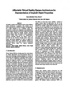
speeds of the two wheels. These are calculated from linear velocity v and angular velocity ω as follows.  ωl = 2v−ωl 2r (4) ωr = 2v+ωl 2r In our experiments, we use p1 = 0.15, p2 = 0.01. The constants used in Eq. 3 are EMP = BE MP = 2.032, and E180 = 1.524, which are computed based on vmax and ωmax . We also choose BE = 0 as we assume there are no errors. The global tick is dt = 0.05s. The update periods of Mission Planning, Navigation, and Inner-Loop & Plant are 4dt, 2dt and dt, respectively. We adopt the algorithm from the Coursera course “Control of Mobile Robots” for the go-totarget controller. The avoid-obstacles controller simply stops the rover, as in [28]. The backtrack controller implements the least-squares approach described in Section IV-B. In Mission Planning, the choose-next-target controller picks the next target in a sequence of pre-determined target locations when the rover arrives at the previous target. The recharge controller simply sets T = PS . Fig. 3 shows the complete trajectory the rover takes with the following configuration. The rover’s starting position is P0 = PS 1 = (−1, 0, 0), its initial heading angle is θ0 = 0, and the targets are T1 = (1.2, 0) and T2 = (0.3, 1.2), which must be visited in that order. The power stations are located at PS 1 = (−1, 0), PS 2 = (0.8, −0.5), PS 3 = (0.4, 0.9). The black lines represent the forward paths and the red line represents the backward path. The rover is able to reach T1 without having to recharge. At position BT = (0.895, 0.570) on its way from T1 to T2 , the battery level drops to B = 29.07, triggering recharge mode. The rover re-traces the forward path segment PS 2 BT exactly (the red and black lines are indistinguishable) to recharge at power station PS 2 . The battery level when it reaches PS 2 is B = 0.07, indicating a tight switching condition. After recharging to full capacity at PS 2 , the rover takes a different path to the last target T2 . A video of the simulation can be viewed at https://youtu.be/i8WGVD5Vk7U.

E. Experimental Results We implemented the CBSA for the Quickbot rover in Matlab using the following parameter values: (1) number of distance sensors N = 8; (2) angle of detection of the sensors βs = 5◦ ; (3) maximum range of the sensors Rs = 0.8m; (7) radius of the wheels r = 0.0325m; (8) distance between the centers of the two wheels l = 0.09925m; (9) maximum linear velocity vmax = 0.8m/s; (10) maximum angular velocity ωmax = 7π rad/s; (11) power station sensor detection range dPS = 0.1m; (12) maximum battery level Bmax = 100. We use a power model that is an affine function of the angular velocities of the two wheels: P (ωl , ωr ) = p1 (|ωl | + |ωr |) + p2 , where p1 and p2 are constants and ωl , ωr are the rotational

Fig. 3. Snapshot from a simulation showing the trajectory the rover takes to visit targets T1 and T2 while ensuring the ES and CF properties.

V. Q UICKBOT M ISSION C OMPLETION The Simplex architecture is not intended for assuring general liveness properties. This is reflected by the fact that a Decision Module looks ahead one update period to determine if the (safety) property in question is about to be violated; as such, it will not be able to detect a violation of a liveness property if the property’s time horizon is unbounded. As we show here, however, the Simplex architecture can be made to work with bounded liveness properties. In particular, we design a CBSA for the Quickbot that assures a property called Mission Completion (MC). Recall that the mission of the Quickbot rover is to visit a sequence of predetermined targets. The MC property ensures that the rover completes its mission within a given amount of time. This property is interesting in the context of Simplex not only because it is a (bounded) liveness property, but also because it is a higher-level mission-oriented property, several layers of control removed from the physical plant. The only physical parameter of the plant in question is (real) time. The MC property is also more software-oriented in nature, as it revolves around a data structure (a list of mission targets). The MC property can be formally expressed as G(F E(p, P S) then B 0 > E(p0 , P S). Since the rover traces through a sequence of recorded waypoints W when going back to P S, we have  E180 + BE (p, P S, W ), if ctlr = AC E(p, P S) = (5) BE (p, P S, W ), if ctlr = BC There are four cases: Case 1: ctlr = BC and ctrl = BC. The rover is in recharge mode. The backtracking energy needed to backtrack from current position p to the next position p0 is BE (p, p0 , W ). Therefore the battery level at the end of the next decision period of MP is (6)

We assume that the ES property holds at current time, i.e., B > BE (p, PS , W )

(7)

We want to prove that the ES property still holds at end of the next decision period of MP i.e., B 0 > BE (p0 , PS , W 0 )

(8)

The backtracking energy from current position p to P S can be partitioned into BE (p, p0 , W ) and BE (p0 , PS , W 0 ), i.e., BE (p, PS , W ) = BE (p, p0 , W ) + BE (p0 , PS , W 0 )

(9)

Re-arranging this equation gives: BE (p0 , PS , W 0 ) = BE (p, PS , W ) − BE (p, p0 , W )

(10)

(11)

(12)

According to Eq. 5, E(p0 , P S) = BE (p0 , PS , W 0 ), therefore: B 0 > E(p0 , P S).

(13)

Case 2: ctlr = AC and ctrl0 = AC. The energy needed to go from current position p to the next position p0 is FE (p, p0 ) ≤ EMP . The battery level at the end of the next decision period of MP is: B 0 ≥ B − EMP (14) We assume that the ES property holds at the current time, i.e., B > E180 + BE (p, PS , W )

Note that if the rover detects a new power station PS on the way from p to p0 then the ES property still holds at the end of the next decision period, because BE (p0 , PS 0 , W 0 ) ≤ BE (p0 , PS , W 0 ). ctrl = AC means the switching condition is false, i.e., B > EMP + E180 + BE MP + (1 + BE )FE (PS , p) (17) Since BE (p, PS , W ) ≤ (1 + BE )FE (PS , p), we have: B > EMP + E180 + BE MP + BE (p, PS , W )

(18)

Combining Eq. 14 with Eq. 18, we have: (19)

BE (p0 , PS , W 0 ) can be partitioned into BE (p0 , p, W 0 ) and BE (p, PS , W ), i.e., BE (p0 , PS , W 0 ) = BE (p0 , p, W 0 ) + BE (p, PS , W )

(20)

0

Energy needed to backtrack from p to p is bounded by BE MP , thus: BE (p0 , PS , W 0 ) ≤ BE MP + BE (p, PS , W )

(21)

Combining Eq. 19 with Eq. 21, we have: B 0 > E180 + BE (p0 , PS , W 0 )

(22)

According to Eq. 5, E(p0 , PS ) = E180 + BE (p0 , PS , W 0 ), therefore, B 0 > E(p0 , PS ). (23) Case 3: ctlr = AC and ctrl0 = BC. The rover is switching from AC to BC, which means it must turn 180◦ before backtracking. The battery level in the next decision period of MP is: B 0 = B − E180 − BE (p, p0 , W ) (24)

B > E180 + BE (p, PS , W )

(25)

We want to prove that the ES property still holds at the end of the next decision period of MP i.e.,

Combining Eq. 6 and Eq. 11, we have: BE (p0 , PS , W 0 ) < B 0

(16) 0

We assume that the ES property holds at the current time, i.e.,

Combining Eq. 7 and Eq. 10, we have: BE (p0 , PS , W 0 ) < B − BE (p, p0 , W )

B 0 > E180 + BE (p0 , PS , W 0 )

B 0 > E180 + BE MP + BE (p, PS , W )

0

B 0 = B − BE (p, p0 , W )

We want to prove that the ES property still holds at the end of the next decision period of MP i.e.,

(15)

B 0 > BE (p0 , PS , W 0 )

(26)

Observe that if we let B180 = B − E180 then Case 3 becomes Case 1 with the same proof. Case 4: ctlr = BC and ctrl0 = AC. When MP switches from BC to AC, the switching condition must evaluate to false, i.e., B > EMP + E180 + BE MP + (1 + BE )FE (PS , p) (27) Thus, this case folds back to Case 2 with the same proof. Proof of hAP i Nav [sNav ] hABE i Since the decision ctlr from MP is hardwired to the switch in Nav, we only need to prove that the backtrack controller

in Nav satisfies BE < (1 + BE )FE (PS , p). As discussed in Section IV-B, the sequence of values of (v, ω) on the backtrack path will have the same magnitudes as the ones on the forward path. Therefore the backtrack energy will be the same as the forward energy. B. Proof of CF Property Proof of hAP i Nav [sNav ] hCF i We prove hAP i Nav [sNav ] hCF i by proving that hAP i AC2 [sNav ] hCF i and hAP i BC2 [sNav ] hCF i. Since AC2 is the same Simplex instance in [28], the proof of hAP i AC2 [sNav ] hCF i is already available there. We show that hAP i BC2 [sNav ] hCF i. Similar to the proof of hAP i Nav [sNav ] hABE i, BC2 will track the forward path exactly, in the reverse direction. Since the forward path is collision-free as guaranteed by the proof that AC2 satisfies the CF property, it immediately follows that the backtracking path is collision-free as well, i.e., hAP i BC2 [sNav ] hCF i.