A Comprehensive Methodology for Vision-Based Progress and Activity Estimation of Excavation Processes for Productivity Assessment Maximilian Bügler1, Gbolabo Ogunmakin2, Jochen Teizer3, Patricio A. Vela2, André Borrmann1 1
Chair of Computational Modeling and Simulation, Technische Universität München, Germany
2
School of Electrical and Computer Engineering, Georgia Institute of Technology, United States of America 3
RAPIDS Construction Safety and Technology Laboratory, United States of America
[email protected]
Abstract. The high level of complexity in modern construction projects causes a-priori project schedules to be highly sensitive to delays in the involved processes. At underground construction sites the earthwork processes are very vital, as most of the following tasks depend on it. This paper presents a novel method for tracking the progress of earthwork processes by combing two technologies based on computer vision: photogrammetry and video analysis. While the former is applied to determine the volume of the excavated soil in regular intervals, the latter is used to generate statistics regarding the construction activities, such as loading times and idle times. Combining these two data sources allows exact measurement of the productivity of the machinery and determining site-specific performance factors. Most importantly, reasons for low productivity – such as an insufficient number of trucks – can be identified easily. The paper presents in detail the vision-based techniques applied and the methods used for combining both data sources. The suitability of the approach has been proved by an extensive case study – a real-world excavation project in Munich, Germany.
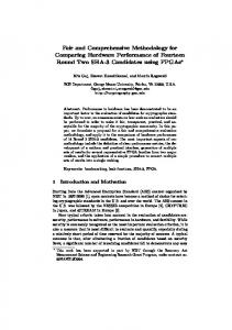
1. Introduction The high level of complexity in modern construction projects causes a-priori project schedules to be highly sensitive to delays in the involved processes. At underground construction sites the earthwork processes are very vital, as most of the following tasks depend on it. Due to the discovery of archaeological artifacts, relocation of undocumented underground utilities, removal of leftover ammunition from wars or pollutants in the soil, impact from adverse weather, and through improper site organization, earthwork processes are often subject to unanticipated delays. These delays are likely to propagate through the entire remaining schedule and adversely impact both progress and productivity. In this paper, we present a novel approach for monitoring earthwork processes using visual sensors for the purpose of extracting activity, progress, and productivity statistics through vision-based processing algorithms. The visual sensors provide both activity and progress data regarding the work site. For the former, a static surveillance camera surveying the primary zone of activity records the ongoing activities. For the latter, visual data in the form of photographs of the work site is obtained on a periodic basis. Figure 1 gives on overview of the combined approach proposed in this paper. On the one hand we apply photogrammetric processing of photo images to determine the earth volume excavated, while on the other hand we perform video analysis to generate statistics regarding the site activates, such as loading times, idle times, and other relevant project management information. Combining these two data sources enables us to exactly measure the productivity 1
of the machinery system and determine site-specific performance factors (Gouett et al., 2011). Most importantly, reasons for low productivity – such as an insufficient number of trucks – can be identified easily. While onsite personnel can notice occurring delays by common sense, the underlying reasons, determined by the described method, can be less obvious.
Figure 1: Data flow diagram of proposed concept
2. Related work Bügler et al. (2013a) presented an approach to estimate the current progress of an excavation process based on determining the excavated volume utilizing photogrammetry and applying the VisualSFM algorithm (Wu, 2011). Ogunmakin et al. (2013) presented a vision-based method for tracking the individual machines involved in the excavation processes and calculating more detailed metrics. These metrics include the idle times of dump trucks, bulldozers, and excavators, the number of dump truckloads observed, and the timespans the dump trucks spend off-site. In this paper, we discuss how these two approaches can be integrated, in order to realize a mechanism for determining the labor productivity. Further analysis of these fused measurements over longer timespans may reveal the causes and time frames of observed delays. Providing feedback of these observations to the worksite stakeholders would allow them to more efficiently be apprised of delays, determine their causes, and react appropriately. Importantly, Gouett et al. (2011) has shown that awareness of labor productivity leads to improvements in the direct work rate, thus the existence of onsite measurement abilities such as those sought in this paper is sufficient to improve onsite operations, irrespective of any adverse conditions that may occur to impede progress. Photogrammetry is increasingly used in many areas of construction projects. Aydin (2014) recently presented a photogrammetric method for façade design and Fathi et al. (2013) presented a method to monitor the fabrication of metal roof panels. Additionally Dimitrov et al. (2014) introduced a method to generate building information models from unordered photographs. Vahdatikhaki et al. (2014) propose to combine different kinds of radio based tracking methods in order to monitor earthwork processes. Pradhananga and Teizer (2013) and Vaseneva et al. (2014) evaluated the use of Global Positioning System (GPS) for such purposes. As Ogunmakin et al. (2013) states, several more researchers are active in this area. 3. Experimental Setup To evaluate the proposed method, we applied both capturing technologies on a single construction site. A video camera was placed on site on a tower crane to record footage of the excavators and dump trucks. Photographs taken from different viewpoints were used for the photogrammetry approach. As the site for the experiment, we chose a new subterranean
2
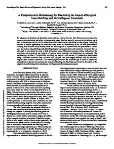
parking lot (see Figure 2) in a particularly confined area of Munich. The site requires a large excavation task to be finished prior to commencing the main building activities. 4. Volume Calculation using Photogrammetry A suitable approach to quantify the amount of excavated soil on an excavation site is to create a three-dimensional (3D) point cloud of the site space (see Figure 3) and use the information to obtain a volume measure. The photogrammetry approach uses photos taken by a pedestrian worker equipped with a conventional digital camera as input data (see Figure 4). Alternatively, a method to record the data using an unmanned aerial vehicle (UAV) system was proposed by Siebert and Teizer (2014). The algorithm locates feature points within the recorded photos using the scale invariant feature transform SIFT (Wu, 2007). Those features are then matched among the individual photographs. Features visible in at least three photographs can then be used to triangulate points in the 3D space (see Figure 3) using the bundler approach published in Wu (2011). Those points eventually form a point cloud. Additionally the patch based multi view stereo (PMVS) algorithm (Furukawa et al., 2010) can be used to create a denser representation of the scene and to add information about normals. In order to calculate the volume of the point cloud, several steps are required. First, the cloud needs to be cleaned from points outside the excavation area, which is performed using cluster analysis. Secondly, a consistent top plane, which covers the excavation area, is found using marker points or a vertical histogram analysis. Furthermore, the top plane is filled with a layer of artificial points with normals facing downwards. Eventually a closed mesh is created using Poisson surface reconstruction (Kazhdan et al., 2006) and the volume of the mesh is calculated using signed tetrahedron volumes. More details on the entire procedure are given in Bügler et al. (2013a).
Figure 3: Point cloud of the excavation site
Figure 2: Layout of construction site subject to the experiments, the diameter is about 50 meters
3
Figure 4: Photographs of the excavation site in the downtown area of Munich, Germany
5. Excavation Tracking using Video Analysis As described in Ogunmakin et al. (2013), an automated system for processing construction site video requires a priori information about the site layout and the proper design of a surveillance system contextualized for the task at hand (in this case the extraction of activity and event statistics of onsite machines). The information required by the system is the work site layout, the machines being tracked, and their process diagrams encoded as a probabilistic graph model (Yang et al., 2013; Ogunmakin et al., 2013). The video processing system consists of four major parts: (1) target detection, (2) target tracking, (3) activity status estimation, and (4) event detection processing. The first part identifies elements in the image that should be tracked. Here, a background model (Stauffer and Grimson, 1999) of an empty scene is used to detect targets within the field of view, especially those that enter the site. When a target is detected, a kernel covariance tracker is initialized for the tracking the target (Yang et al, 2010; Ogunmakin et al., 2013). The role of the tracker is to maintain a consistent temporal trajectory for the detected target over time. While the targets are being tracked, the activity status for each machine, moving or static, is estimated. The activity status estimator also estimates whether an excavator is filling a dump truck or not. The event detection processor combines the output from the tracker and the activity status estimator to generate detailed metrics regarding important onsite events. Figure 5 shows the process flow of the automatic system. For the system to work, the stationary video camera providing the visual stream must be mounted in a position that provides a field-of-view large enough to capture the work area of all machines of interest. Tower crane mast, roofs of nearby buildings or structures, or other temporary construction facilities offer good locations as long as they do not move much (Bohn and Teizer 2010).
Figure 5: Process flow for the automatic surveillance system
5.1 Target Detection Target detection utilizes a background Gaussian Mixture Model (GMM), which identifies anomalies in the image relative to an expected background image (Stauffer and Grimson, 1999). The initial background model comes from the estimation technique proposed by Reddy et al. (2009). Targets detection is performed by computing the probability of each pixel belonging to the background. Regions with low probabilities below a threshold result in a foreground mask giving all foreground items in the scene. This information is coupled with the work site layout information (e.g., entrance gates or zones) to determine when a target
4
first enters the scene. Figure 6 depicts the primary background model (the strongest mixture element for each pixel), a sample image from surveillance video, and the foreground regions.
Figure 6: From left to right: sample estimated background, sample image, and foreground detection
5.2 Kernel Covariance Tracking The kernel covariance tracker used in this work is an improvement on the tracker proposed by Yang et al. (2010). Several improvements are made: (1) reduction of data before tracking (Kingravi et al., 2013) and (2) introduction of a scale space search with upper limits and lower limits. The data reduction step saves memory and lowers the computational cost of tracking. The scale space search allows the tracker to handle changes in scale. To initialize the tracker, the target’s color and spatial information are learned through kernel principal component analysis (KPCA) with a Gaussian kernel. For every frame and each target, a gradient ascent procedure localizes the target by comparing the foreground image data with the targets’ learned model. Figure 7 depicts the tracking results for a short segment of time. The three targets are outlined by a bounding box and their trajectories into the future are depicted.
Figure 7: Sample kernel covariance tracking results
5.3 Activity Status Estimation The activity status of the machines follows that of Ogunmakin (2013), where machine activity is decomposed into static, moving, or within a region of interest. Each region of interest has specific meaning as derived from the probabilistic graph model of the potential activity states of each machine. An additional activity check is performed when an excavator and a dump truck are in close proximity. Then, much like in Golparvar-Fard et al. (2013), where the movement of the excavator’s spatio-temporal features provides an indication of excavator activity, the movement of the excavator in the proximity zone of a dump truck establishes 5
when an excavator is filling a dump truck. This state can only be triggered when the two machines are in close proximity and the dump truck is static. 5.4 Event Detection Processor The event detection processor takes as input, the trajectory information from the tracker and the results from the activity status estimation, and uses this to generate the statistics needed to determine the timespans of the work activities of the excavators and dump trucks. The metrics computed are the number of dump trucks that entered the scene, how much time they spent in the region of interest getting filled, how many bucket loads of soil were placed in each dump truck, and how long the machines spent idle while in the scene. Figure 9 depicts the output of the event detection processor, which includes a display of the aggregate statistics, Figure 9(a), and a table with the temporal breakdown of the activity states, Figure 9(b). In addition, robust estimation is used to estimate activity averages and identify outliers (discussed in results).
Figure 8: Dump truck state estimates for a video segment. The activity states are static (red), moving (green), filling (magenta), and absent (blue). Initially a dump truck is in the scene, then leaves (2 minute mark). Another enters (near 3 minute mark) and is then filled by the excavator. Truck Load (No.) 3 4
Entered Site at Minute 26.75 32.85
Moving (Mins)
Static (Mins)
Filling (Mins)
0.36 0.59
3.2 1.35
1.43 2.06
(a) Sample pie chart
Exited Total on # of Site at Site Buckets Minute (Mins) to Load 31.74 4.99 8 36.85 3.99 9
(b) Sample event statistics table
Figure 9: Event analysis and statistics for a video segment. The event processor tabulates the temporal statistics of the activities and also identifies events, such as filling cycles and outlier time spans. For the analysed timespan, the pie chart on the left indicates what percentage of the time was spent engaged in which activity state. The activity states are static (red), moving (green), filling (magenta), and absent (blue). The sample table on the right depicts the activity analysis breakdown based on the frames analysed
6. Data Consolidation Both data sources are utilized to observe the site. The excavated volume is measured on a regular basis using the photogrammetry approach. At the same time, all excavation processes are recorded using a stationary video camera. Whenever a delay in excavation is observed, the video analysis is used as a tool to determine the cause of the delay; as the video analysis gives rise to idle times of the individual machines. Charts like the one visualized in Figure 9 are 6
used to categorize the events recorded in the video by means of different machine states. If excavation is particularly slow in a certain time span and there are extended periods of absent dump trucks at the same time, this can indicate that trucks might be stuck in road traffic jams or are not sequenced timely enough. Alternatively, it is possible that the overall number of used dump trucks is too low and it would be useful to hire additional trucks. In the contrary case, where dump trucks are waiting a long time to be filled, it is likely that either too few excavators are used or too many trucks are in use. Other reasons can be site congestion, when equipment or other obstacles (e.g., as-built structures or temporary placement of objects) cause delays because of complex on site traffic patterns. Whenever the site allows for placing more excavators, this is worth consideration, when the deadlines for the excavation processes are in jeopardy and the cost of hiring additional excavators does not exceed the costs for possible schedule delays and potential penalties. 7. Results A period of 4 hours was recorded on video during excavation of the site described in Section 3, while two point clouds were created before and after the recording period. The point clouds are illustrated in Figure 10. As the time period was comparatively short, the difference is minimal but visible on the left side of the pit next to the excavator. The video camera was positioned on a tower crane during the recording in order to have an overview of both excavators and dump trucks. A screenshot of the recorded video was shown in Figure 7. The analysis of the video indicates some periods of idle machinery and available time. Table 1 contains a breakdown of the time statistics for the 22 filling cycles detected in the 4 hours period of video recorded. These statistics were used to generate several graphs automatically (in Matlab). The chart of aggregate statistics, Figure 11(a) indicates that only 39% of the available filling time was used. It is therefore possible to improve on the efficiency of the process by incorporating more dump trucks to reduce the idle times of the excavators and increase the amount of soil removed from the site. The filling time per dump truck averaged 3.65 minutes with five identified outliers (taking 4.8 minutes or more; marked in orange in Table 1). The estimated total amount of time the dump trucks were in the scene was 88.33 minutes (out of 240 minutes of video). Additionally, the inter-arrival time between dump trucks was measured to be 3.21 minutes on average (excluding the automatically identified outliers), with the estimated total inter-arrival time for the dump trucks being 144 minutes, see Figure 12. The outlier times (there are six of them totalling about 105 minutes) consist of periods when the excavators are doing support work, or are idle.
Figure 10: Point clouds of excavation site before and after video recording
7
(a) Pie chart with aggregate statistics
(b) Time spent per dump truck in the scene
Figure 11: Aggregate dump truck states for the entire video sequence (left) and dump truck filling time estimates per truck (right): (a) Indicates what percentage of total recording time the associated work states were observed. (b) Total time each dump truck spent in the scene. The red line is the average time spent in the scene. The average represents the typical amount of time spent to load and prepare the dump truck (the excavator spends some time levelling the soil in the filled truck bed).
Figure 12: Inter-arrival times between the dump trucks. The inter-arrival time is the time duration between when the previous dump truck leaves and the next dump truck enters. For the first dump truck, the time quantity measures the amount of time from the start of the video to when the dump truck first entered. The red line is the average of the inter-arrival times, after excluding the larger outlier times. This average represents the typical amount of time between when a dump truck exits and another enters for a relatively continuous stream of dump trucks (for this observed video sequence).
Figure 13: Performance factor and cumulative soil removed (units are in cubic meters). Soil removal progress is per hour (left) and cumulative soil removed is per 10 minute interval.
The statistics from Table 1 combine with the progress results to provide estimates of the average quantity of soil removed per truck and the average quantity of soil per bucket load, either of which can be used to estimate the productivity of the earth removal process. According to the photogrammetry estimates, the total quantity of soil removed was 417.90 cubic meters. Given that 22 dump trucks were filled, the average volume of soil per dump truck was 19 cubic meters. For the 171 bucket loads detected to have occurred, the average 8
bucket load removed 2.44 cubic meters. Total amount of onsite activity was 134.33 minutes. These averages and the data from Table 1 inform progress statistics calculations that are performed automatically. Figure 11 depicts the volume of soil removed per hour of observation, and the cumulative soil removed over the course of the observations. Project schedule management could benefit from the generated information in multiple ways given near-real-time processing and availability: (1) hire more trucks to complete excavation quicker, (2) increase the contingency available for succeeding activities, (3) learn and add to historic schedule estimates, (4) and apply in future projects considering lean principles. Table 1: Statistics for each truck that entered the scene. Truck Load (No.) 1 2 3 4 5 6 7 8 9 10 11 12 13 14 15 16 17 18 19 20 21 22 Total
Entered Site at Minute 14.57 20.29 26.75 32.85 38.60 44.09 50.07 69.13 74.39 79.27 87.79 96.01 102.79 108.15 112.95 119.07 131.31 138.03 152.77 165.69 172.65 229.14
Moving (Mins)
Static (Mins)
Filling (Mins)
0.17 0.41 0.36 0.71 0.15 0.22 0.35 0.15 0.15 0.13 0.72 0.15 0.55 0.15 0.15 0.19 0.14 0.17 0.27 0.13 0.45 0.29 6.15
2.42 2.72 3.20 1.45 1.50 1.73 1.57 1.04 1.52 1.87 2.91 3.63 1.89 1.19 1.67 0.86 2.52 0.81 1.94 1.59 1.38 1.35 40.76
1.84 2.05 1.43 1.84 1.57 1.81 1.64 1.68 1.56 2.00 1.40 1.47 1.02 1.97 1.68 1.57 1.65 1.47 1.35 1.63 0.89 0.84 34.35
Exited Site at Minute 19.01 25.46 31.74 36.85 41.87 47.94 53.77 72.17 77.84 83.53 93.11 101.58 106.63 111.87 116.91 122.19 136.15 141.06 156.93 169.69 176.06 232.35
Total on Site (Mins) 4.43 5.17 4.99 3.99 3.27 3.85 3.69 3.04 3.45 4.25 5.33 5.57 3.84 3.72 3.96 3.11 4.84 3.03 4.17 4.00 3.41 3.21 88.33
# of Buckets to Load 8 10 8 9 9 9 7 8 6 8 9 8 9 9 8 7 7 7 6 6 7 6 171
8. Conclusions The proposed method combines two state of the art procedures to observe excavation processes by video recordings of the involved machinery and photographs of the excavation site. While the photogrammetry approach keeps track of the excavated volume of the pit, the video analysis serves as a tool to provide activity and event statistics. Combining the two provides a means to perform productivity analysis in an automated manner. The determined performance factors provide an excellent basis for calculating future projects with similar conditions. Furthermore, the activity and event statistics can be analysed to identify the causes of observed delays and prevent them in the future. If needed, the time stamps of the observations can be used to quickly review specific segments of video to aid in the analysis. 9. Acknowledgements Parts of the research presented have been funded by the Bavarian Research Foundation within the frame of the project FAUST, and by the National Science Foundation (CMMS #1030472). Their support is gratefully acknowledged. 9
10. References Aydin, C.C. (2014). Designing building façades for the urban rebuilt environment with integration of digital close-range photogrammetry and geographical information systems. Automation in Construction, Elsevier, 43, pp. 38–48, 2014. Bohn, J.S. and Teizer, J. (2010). Benefits and Barriers of Construction Project Monitoring using Hi-Resolution Automated Cameras. ASCE J. Construction Engineering and Management, 136(6), pp. 632-640. Bügler, M., Metzmacher, H., Borrmann, A., and Treeck, C.V. (2013a). Integrating Feedback from Image Based 3D Reconstruction into Models of Excavation Processes for efficient Scheduling. Proceedings of the EGICE Workshop on Intelligent Computing in Engineering, Vienna, Austria. Bügler, M., Dori, G. and Borrmann, A. (2013b). Swap Based Process Schedule Optimization using DiscreteEvent Simulation. Proceedings of the International Conference on Construction Applications of Virtual Reality (CONVR), London, United Kingdom. Dimitrov, A. and Golparvar-Fard, M. (2014). Vision-based Material Recognition for Automated Monitoring of Construction Progress and Generating Building Information Modeling from Unordered Site Image Collections. Advanced Engineering Informatics, Elsevier, 28(1), pp. 37–49, 2014. Fathi, H. and Brilakis, I. (2013). A videogrammetric as-built data collection method for digital fabrication of sheet metal roof panels. Advanced Engineering Informatics, Elsevier, 27(4), pp. 466–476, 2013. Furukawa, Y., & Ponce, J. (2010). Accurate, dense, and robust multiview stereopsis. Pattern Analysis and Machine Intelligence, IEEE Transactions on, 32(8), 1362-1376. Golparvar-Fard, M., Heydarian, A., and Niebles, J. (2013) “Vision-Based Action Recognition of Earthmoving Equipment Using Spatio-Temporal Features and Support Vector Machine Classifiers.” Advanced Engineering Informatics, Elsevier, 27, pp. 652-663. Gouett, M., Haas, C., Goodrum, P., and Caldas, C. (2011). “Activity Analysis for Direct Work Rate Improvement in Construction.” ASCE J. Construction Engineering Management, 137(12), pp. 117-1124. Kazhdan, M., Bolitho, M., and Hoppe, H. (2006). Poisson surface reconstruction. In Proceedings of the 4th Eurographics symposium on Geometry processing. Kingravi, H., Vela, P.A., and Grey, A. (2013). “Reduced Set KPCA for Improving the Training and Execution Speed of Kernel Machines.” SIAM Int. Conf. on Data Mining. Austin, TX. Ogunmakin, G., Teizer, J. and Vela, P.A. (2013). Quantifying Interactions Amongst Construction Site Machines. Proceedings of the EG-ICE Workshop on Intelligent Computing in Engineering, Vienna, Austria. Pradhananga, N. and Teizer, J. (2013). Automatic Spatio-Temporal Analysis of Construction Equipment Operations using GPS Data. Automation in Construction, Elsevier, 29, pp. 107-122. Reddy, V., Sanderson, C., Lovell, B. (2009). “An Efficient and Robust Sequential Algorithm for Background Estimation in Video Surveillance.” IEEE Int. Conf. on Image Processing. 1109-1112. Cairo, Egypt. Siebert, S. and Teizer, J. (2014). Mobile 3D mapping for surveying earthwork projects using an Unmanned Aerial Vehicle (UAV) system. Automation in Construction 41, pp. 1-14. Stauffer, C., Grimson, W.E.L., (1999). “Adaptive Background Mixture Models for Real-Time Tracking,” In: Second IEEE Workshop on Visual Surveillance. Vahdatikhaki, F. & Hammad, A. (2014). Framework for near real-time simulation of earthmoving projects using location tracking technologies. Automation in Construction, Elsevier, 42, pp. 50–67, 2014. Vaseneva, A., Pradhananga, N., Bijlevelda, F.R., Ionitac, D., Hartmann, T., Teizer, J., and Dorée, A.G. (2014). An Information Fusion Approach for Filtering GNSS Data Sets Collected During Construction Operations. Advanced Engineering Informatics, Elsevier. Wu, C. (2007). SiftGPU: A GPU implementation of Scale Invariant Feature Transform (SIFT). University of North Carolina at Chapel Hill. Wu, C. (2011). VisualSFM: A Visual Structure from Motion System. URL http://www.cs.washington.edu/homes/ccwu/vsfm. Yang, J., Arif, O., Vela, P. A., Teizer, J., and Shi, Z. (2010). “Tracking Multiple Workers on Construction Sites using Video Cameras.” Advanced Engineering Informatics, Elsevier, 24(4), pp. 428-434. Yang, J., Vela, P.A., Teizer, J., and Shi. Z. (2013). “Vision-Based Tower Crane Tracking for Understanding Construction Activity.” ASCE Journal of Computing in Civil Engineering, 28(1), pp. 103-112, 2013.
10