A COMPRESSION METHOD FOR ARBITRARY PRECISION FLOATING-POINT IMAGES Steve Mann
Corey Manders, Farzam Farbiz
Dept. of Electrical and Computer Eng. University of Toronto, 10 King’s College Rd, Toronto, Canada
[email protected]
A*STAR Institute for Infocomm Research 21 Heng Mui Keng Terrace, 119613, Singapore {cmanders, farbizf}@i2r.a-star.edu.sg
ABSTRACT The paper proposes a method of compressing floating-point images of arbitrary precision. The concept of floating point images is used frequently in such areas as high dynamic range imaging, where pixel data stored as 8 or 12-bit integers are insufficient. The compression scheme presented in the paper organizes the floating point data in a manner such that already existing compression algorithms such as JPEG or Zlib compression may be used once the data re-organization has taken place. The paper compares the result to a popular (but restrictive) form of image compression, openEXR, and shows significant gains over this format. Furthermore, the compression scheme presented is scalable to deal with floating point images of arbitrary precision.
compression, as the application to lossy compression and its comparison to other methods is the subject of ongoing research. Thus the comparison to the openEXR format is only done for lossless compression. The method as presented may be applied to decimated chrominance channels, different colorspace representations, or different floating point representations with ease. The implementation as presented represents a significant improvement over the authors previous work (see [7]).
Index Terms— Image Analysis, Image Coding, Floating Point Arithmetic, Image Processing, Imaging. 1. INTRODUCTION: MOTIVATING FLOATING POINT IMAGES Typical images taken using digital cameras capture scenes of low dynamic range. In the past, this was largely the result of inadequacies in both equipment used to capture the data as well as the means of display for these images. For example, someone taking an image of a person outside will generally point a camera away from the sun. In essence, what this does is reduce the dynamic range of the scene. Given typical camera equipment and its limitations, this will result in a more pleasing low dynamic range image. However, given the possibility of high dynamic range images [1] [2], as well as high dynamic range displays [3] high dynamic range images are now possible. Unfortunately, previous file formats lack the capability to store the dynamic range needed. Though other work has been done on storing data as integer values with a greater range [4], the same work notes that the “obvious choice” to encode luminance is “using floating point values”. In such work, the authors choose not to encode data in floating point numbers because of the problems inherent in compressing floating point numbers. One significant design detail should be mentioned about our compression format, specifically that it is a general method of compressing floating point images. In other work (such as [5] and [6]) there is an assumption that the images are to be viewed by humans at a specified intensity. Given this criterion, the chrominance of the image may be compressed more heavily than the luminance. This of course results in greater compression (with loss), but is largely unnoticed by viewers. The results we present are only in regards to lossless compression, although it shall be shown how lossy compression may be applied. We limit the scope of this paper only to lossless
1-4244-1437-7/07/$20.00 ©2007 IEEE
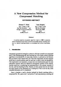
Fig. 1: The top row shows two low dynamic range images taken at both short and long exposure times. The two low dynamic range are composited to produce a single high dynamic range image. Notice that in the short exposure time image (top left), the shape of the bulb is evident, the position of the filament, etc. However, much of the information of the scene is lost. For example, the flowers to the right of the halogen light are not seen. Conversely, if we look at the long exposure time image (top right), the flowers are present, however, much of the information of the bulb is lost. The bottom row shows a single high dynamic range image in a simple image viewing program. The bottom left image shows the HDR at a gain approximately equal to the input image shown at the top left, and the bottom right image shows the HDR image at a gain approximately equal to the input image shown at the top right. The bottom center image is the high dynamic range image at an intermediate gain, in effect producing an interpolated exposure. Note that the bottom row depicts a single HDR image shown at three different gains. The spatial resolution of the input images is 1520 × 1007 and uses three color channels (red, green, and blue) which results in a floating point image size of 17.5Mb using IEEE single precision floating point representation.
2. CREATING HDR IMAGES The test images which were used for our study were derived by very simple means. Specifically, many digital SLR cameras now available provide raw sensor data (for example Nikon and Canon digital SLR cameras). This data has been shown to be linear in response to the amount of light detected [8][9]. To build a high dynamic range image, multiple exposures of the high dynamic range scene were taken. The exposure times used were all possible exposure times available on the digital camera within reason. For example, there is no sense capturing a 25 second exposure of the scene if this will result in all
IV - 165
ICIP 2007
3. THE COMPRESSION STRATEGY In this section we will motivate and describe our method for compressing floating point image files. 3.1. Distribution of extended dynamic range data The same image that was used in the previous section (figure 1) for demonstration will continue to be the primary example. However, the results of the findings will be applied to multiple images in a future section. Given that it makes most sense to represent a lightspace image value (flat response pixel) as a floating point number, we first look at a typical distribution of data. Because the demonstration image does in fact capture a wide dynamic range and is represented in floatingpoint values, plotting the distribution of values makes little sense. Thinking ahead as to what the data looks like from the viewpoint of compression, it makes more sense to look at the distribution of mantissas and exponents. Figure 2 shows the distribution of the mantissas and exponents for the extended dynamic range image presented in figure 1. 3.2. Considering pixel differences In the case of the distributions shown in figure 2, the mantissas in particular are close to being uniformly distributed. For this reason, the values are not easily compressible. However, if we consider differences of neighbouring pixels, the distributions change dramati-
2
Distribution of Mantissas
Distribution of Exponents
x 104
250
1.8 1.6
200
1.4
150
Count
Count
1.2 1
0.8
100
0.6 0.4
50
0.2 0 4
6
8
10
12
14
16
−x Exponent 2
18
0 0
20
1
2
3
4
5
6
7
8
Mantissa of the photoquantity
9 x 10⁶
Fig. 2: Distribution of exponents (left) and mantissas (right) for the extended dynamic range shown in figure 1. Note that the distribution of mantissas is largely uniform. Note that the histogram of the mantissas is truncated at 223 = 8388608 as the IEEE Standard 754 floating point representation allows for 23 bits of data in the mantissa, 8 bits of data in the exponent, and 1 sign bit. Distribution of Successive Pixel Differences in Exponents 4
9
Distribution of Successive Pixel Differences in Mantissas
x 10
1800
8
1600
7
1400
6
1200
5
1000
Count
Count
pixels being saturated. Consequently, there is no point in capturing images which will only result in dark current noise [10]. It is also known that sensors, including imaging sensors, are most accurate in the higher end of reported values before saturation occurs [11]. Given these observations, we would like to use pixels in the RAW images which were captured in this range of the camera’s capabilities. To do this, for each pixel location, the pixel value that was used was that which belonged to the exposure which produced a pixel in this desired range (for the images in this paper, the range [0.65,0.9] was taken. The value was then divided by the appropriate scalar to bring the pixel value into that of the lowest exposure. Therefore, if the resulting extended dynamic range image is multiplied by this scalar, the resulting pixel value will be that of the original image. In the case where multiple exposures produced more than one candidate value for a single location, all values were divided by their corresponding scalar to bring the values to the lowest exposure, and the resulting values were averaged. Figure 1 shows two of the many images used to create a single extended dynamic range image. Using an appropriate image viewer, these exposures may be recreated from the resulting high dynamic range image. Though a rectangular weighting (also called certainty [11]) function in the case of figure 1 was used, many other possibilities exist. Using a rectangular function is very easy to compute and use, however it is susceptible to changes in lighting, camera movement, or minute scene changes. Other work has used a center weighted function [2] or more appropriately a right-skewed Gaussian function [12], which favors high photoquantities and reduces noise in the final image. The right-skewed rectangular function was used because most of the images were taken in well controlled environments. In situations where the environment is uncontrolled (for example there exists movement in the image as well as movement in the position of the camera), previous research [1] [13] shows that HDR images may also be produced.
4
400
2
200
1 0 −5
800 600
3
−4
−3
−2
−1
0
1
2
3
4
5
Successive pixel difference
0 −1
−0.8
−0.6
−0.4
−0.2
0
0.2
0.4
Successive pixel difference
0.6
0.8
1 7
x 10
Fig. 3: Distribution of horizontal pairwise pixel differences in exponents (left) and mantissas (right) for the extended dynamic range image shown in figure 3. Note that the distributions have now become zero centered with a high falloff.
cally. This largely comes from an expectation that given an arbitrary pixel, the pixels in its neighbourhood will be similar. Thus differences will largely be zero. This is confirmed in the plot shown in figure 3, where successive value differences are used. 3.3. Pixel differencing scheme used for compression To utilize the benefit of pixel differencing, the differencing scheme shown in figure 4 was used. This scheme assumes that neighbouring pixels will be similar. So that the first column of values in the image are not all large (since there is no value to the left to create a difference), the difference to the value directly above is used. Thus, if all pixels in the image are roughly similar, the only large value to be stored in the image is the value stored in the top left corner. The scheme may easily be defeated. For example, if a checkerboard image was created where neighbouring pixels were dramatically different, there would be no savings in this scheme. In fact, the differencing scheme would result in an image which would likely take more space to store (assuming LZW or zlib compression is used). Just as JPEG compression assumes “natural” images, we consider images such as pixel-wide checkerboard patterns unnatural and unlikely. 3.4. Expanding value differencing Differencing in terms of the image presented in figure 1 works tremendously well in terms of the exponent. To demonstrate this, this image was compressed by splitting the exponents and mantissas. Single-precision floating point numbers were used with the usual IEEE specification of three bytes allocated to the mantissa and one byte allocated to the exponent. The differencing scheme was also
IV - 166
Fig. 4: The differencing scheme using to reduce the overall size of the values to be represented in the extended dynamic range image. Note that the original light values are always used. Thus, the value stored in position l3 is the value l3 − l0 . The value stored in position l1 is l1 − l0 .
Component Exponent Low Byte Middle Byte High Byte
Uncompressed Size 4484.4Kb 4484.4Kb 4484.4Kb 4484.4Kb
Compressed Size 604.7Kb 3981.8Kb 3720.9Kb 2353.3Kb
Table 1: The resulting sizes of each compressed component using byte image differences. The resulting lossless compressed file is 10660Kb rather than the original file size of 17937.2Kb. This represents a 40% savings in file size.
utilized. The resulting exponents were compressed from 4484.4Kb to 604.7Kb. However, the mantissas compress from 13453.2Kb to 11084.4Kb. This implies a 86.5% savings in the exponent and only a 17.6% savings in the mantissa. Following the similar neighbouring pixel idea, it is reasonable to assume that the first bytes of neighbouring values mantissas will be similar, and to a lesser extent, the lower order bytes will contain similarities. Using this logic, the three orders of bytes were compressed separately. The method can be thought of as first separating the image into mantissa and exponent images, and then splitting the mantissa image into high-byte, mid-byte, and low-byte images. We have stored and processed the file as a single-precision floating point value for simplicity. The byte decomposition scheme is of course easily applied to double-precision floating point values, or, floating point representations of higher precision. Using zlib (see http://www.zlib.net) compression on each of the four bytes, the images were written to a single file. The component sizes shown in Table 1 were observed. Note that to aid in the overall compression, the byte images for each color channel were ordered sequentially. That is, a single array was created from first the red, green, and blue high-byte mantissa images, then the middle-byte color images, then low, then the red, green, and blue exponent images. By grouping like colors, and like floating point bytes together, the array could be easily reconstructed into the original floating point image. However, the array also successfully groups similar components together.
Fig. 5: Images used to test the floating-point compression scheme. As well the HDR image shown in figure 1 was also used. The HDR images in the set are shown at a low gain (left) and a high gain (right). Each row is one HDR image shown at a low (left) and high (right) gain.
is available at [14]. The results of each form of compression on the test images are shown in table 2. As one may observe from the table, the savings over the openEXR format is between 16 − 22%. The compression strategy presented offers some other advantages given the one byte groupings used. Specifically, many existing image compression routines are designed for 8-bit (one byte) data. For example, JPEG compressors are most often written expecting data in this form. Thus, already existing compression strategies may be applied to each of the byte images. The organization into onebyte high, medium, and low mantissa and exponent images allows the zlib compression which was used for the lossless encoding of each byte image to be easily implemented (to see the code used, look at www.eyetap.org/∼corey/code.html). We also applied varying lev-
Image 4. TEST SET AND RESULTS Using the method described previously to capture high dynamic range scenes, the images shown in figure 5 were composited from several low dynamic range images to produce a single high dynamic range image. As well as applying our compression scheme as described to the HDR images in 5 and 1, the images were compressed using openEXR’s format. To be able to judge the differing compression schemes on an equal footing, code was written using the openEXR libraries to write out .exr files with red, green, and blue colour channels. Each colour channel was written out as 32-bit single-precision floating point data. The code which was used to perform this action
Flowers Plant Sun Flashlight Bike
Raw Floating Point 18Mb 18Mb 18Mb 70Mb 18Mb
Open EXR 14Mb 13Mb 15Mb 63Mb 16Mb
Proposed Scheme 11Mb 11Mb 12Mb 50Mb 13Mb
Improvement Over openEXR 16.5% 16.8% 20.8% 21.4% 20.0%
Table 2: Results of compressing five HDR files with openEXR as well as the proposed strategy. The flashlight image was composed using the technique presented, but from low dynamic range base images of spatial resolution 3038 × 2012, whereas all other images used base files of spatial resolution 1520 × 1007. The “improvement over openEXR” column was computed directly from the byte counts of the resulting files. Note that the first image (Flowers) appears in figure 1, where as the following four high dynamic range images appear in figure 5.
IV - 167
els of JPEG compression to the low order mantissa image, and were able to further compress the HDR images without any noticeable difference (applying JPEG compression to all other byte images did produce artifacts as the quantization was increased). We have not reported these compression results as the topic is beyond the scope of this article, and, it is likely that this loss of precision could be significant to computations on the HDR image. For the present topic, we restrict ourselves to lossless compression. We only wish to suggest that the scheme allows for the possibility of lossy compression using existing tools. 4.1. The value of more bits One criticism that may come up in regard to the 32-bit IEEE floating point precision used is that it uses more bits than are necessary to span the dynamic range of the human eye (the exponent uses one byte), and, uses more bits than are necessary to represent increments that are just under the just noticeable difference (JND) of the human eye (the mantissa uses three bytes). Though this is certainly true: • The scheme is presented as a general strategy. It is completely conceivable that one may want to record images beyond the range of the human eye, or, for that matter, with discrete increments far below that of the just noticeable difference of the human eye. • A high precision format is appropriate as an intermediate format during processing of the image. This is comparable to “guard bits” commonly used in microprocessors. • In the case of using a high number of bits where a lower number may be necessary, after the differencing is performed on the data, the unnecessary bytes in the mantissa and exponent will mostly be zero. Thus these bits will compress extremely well. • The compression strategy is easily scaled down to less bits (for example the NVidia half-precision or fp16 format). 5. CONCLUSION We have presented a compression strategy for floating-point images. We have also shown a very simple means of producing high dynamic range images given a scene with a large dynamic range. For the majority of the paper, the data used was single-precision IEEE floating-point representation. This choice made the comparison to the openEXR format rather simple. Aside from the compression improvement over openEXR (shown in table 2), the strategy has several other benefits over openEXR. Specifically, the scheme is scalable to any floating point precision. In addition, it may be scaled down to use the NVidia half-precision format. Given the expansion of the precision to any number of bits, the scheme makes no assumptions about the dynamic range of the images. Other formats assume that the dynamic range is limited to that of the human eye (for example [4] [6] [15], or the openEXR format used for comparison in this work). Additionally, the compression strategy is easily expandable to lossy compression given that already developed techniques may be applied. To this end, the possibility of compressing the low order byte using JPEG compression was suggested. This however is not the end of the possibilities. The low order byte image, the most random and hardest to compress of the bytes, may be compressed in a lossy manner using any number of techniques (even simple quantization). The means of further compressing the low order byte, or for that matter any of the bytes, is a complex and subjective issue dependent upon how the image will be used.
What has been presented is an overall scheme which has tremendous advantages. After separating the floating-point representation into 8-bit sections, the resulting byte images were then grouped together and losslessly compressed using zlib compression. 6. REFERENCES [1] S. Mann and R.W. Picard, “Being ‘undigital’ with digital cameras: Extending dynamic range by combining differently exposed pictures,” in Proc. IS&T’s 48th annual conference, Washington, D.C., May 7– 11 1995, pp. 422–428, Also appears, M.I.T. M.L. T.R. 323, 1994, http://wearcam.org/ist95.htm. [2] P. E. Debevec and J. Malik, “Recovering high dynamic range radiance maps from photographs,” SIGGRAPH, 1997. [3] H. Seetzen, W. Heidrich, W. Stuerzlinger, G. Ward, L. Whitehead, M. Trentacoste, A. Ghost, and A. Vorozcovs, “High dynamic range display systems,” SIGGRAPH, 2004. [4] Rafal Mantiuk, Grzegorz Krawczyk, Karol Myszkowski, and HansPeter Seidel, “Perception-motivated high dynamic range video encoding,” ACM Trans. Graph., vol. 23, no. 3, pp. 733–741, 2004. [5] Ruifeng Xu, Sumanta N. Pattanaik, and Charles E. Hughes, “Highdynamic-range still-image encoding in jpeg 2000,” IEEE Comput. Graph. Appl., vol. 25, no. 6, pp. 57–64, 2005. [6] Greg Ward and Maryann Simmons, “Jpeg-hdr: A backwardscompatible, high dynamic range extension to jpeg,” November 7-11, 2005. [7] Steve Mann, Corey Manders, Billal Belmellat, Mohit Kansal, and Daniel Chen, “Steps towards ’undigital’ intelligent image processing: Real-valued image coding of photoquantimetric pictures into the jlm file format for the compression of portable lightspace maps,” Proceedings of ISPACS 2004, Seoul, Korea, Nov. 18 - 19, 2004. [8] C. Manders, C. Aimone, and S. Mann, “Camera response recovery from different illuminations of identical subject matter,” in Proceedings of the IEEE International Conference on Image Processing, Singapore, Oct. 24-27 2004, pp. 2965–2968. [9] C. Manders and S. Mann, “Determining camera response functions from comparagrams of images with their raw datafile counterparts,” in Proceedings of the IEEE first International Symposium on Intelligent Multimedia, Hong Kong, Oct. 20-22 2004, pp. 418–421. [10] D. Yang, B. Fowler, A. El Gamal, H. Min, M. Beiley, and K.Cham, “Test structures for characterization and comparative analysis of CMOS image sensors,” Proc. SPIE, vol. 2950, pp. 8–17, October 1996. [11] Steve Mann, Intelligent Image Processing, John Wiley and Sons, November 2 2001, ISBN: 0-471-40637-6. [12] S. Mann, “Comparametric equations with practical applications in quantigraphic image processing,” IEEE Trans. Image Proc., vol. 9, no. 8, pp. 1389–1406, August 2000, ISSN 1057-7149. [13] F.M. Candocia and D. Mandarino, “A semiparametric model for accurate camera response function modeling and exposure estimation from comparametric data,” IEEE Transactions on Image Processing, vol. 14, no. 8, pp. 1138–1150, August 2005, Avail. at http://iul.eng.fiu.edu/candocia/Publications/Publications.htm. [14] Corey Manders, ,” http://www.eyetap.org/∼corey/code.html. [15] Gregory Ward Larson, “Logluv encoding for full-gamut, high-dynamic range images,” Journal of Graphic Tools, vol. 3, no. 1, pp. 15–31, 1998.
IV - 168