A Computational Approach to Statistical Inferences - CiteSeerX

Journal of Applied Probability & Statistics c °2007 Dixie W Publishing Corporation, U. S. A.

Vol. 2, No. 1, 13-35

A Computational Approach to Statistical Inferences Nabendu Pal Department of Mathematics, University of Louisiana at Lafayette, Lafayette, Louisiana 70504, U. S. A. Email: [email protected]

Wooi K. Lim Department of Mathematics, William Paterson University, Wayne, New Jersey 07470, U. S. A. Email: [email protected]

Chia-Hua Ling Department of Accounting, Shih Chien Univeristy, Taipei 104, Taiwan, R. O. C. Email: [email protected] Abstract The purpose of this paper is to provide a step by step computational approach to handle statistical inferences based on a parametric model for a given data set. This approach may come handy in those cases where the sampling distributions are not easy to derive or extremely complicated. Our suggested approach provides an algorithmic framework based on the Monte-Carlo simulation and numerical computations which can be implemented mechanically by applied researchers to draw statistical inferences when a suitable parametric model is assumed for a given data set. As a demonstration our proposed method is applied to two real life data sets to show how easily it can be implemented, and in terms of power it can be as good as (if not better than) the other reported method(s). Keywords: Hypothesis testing, interval estimation, power. 2000 Mathematics Subject Classification: 62F03, 62F25, 62E17.

1 Introduction Recent advances in mathematical and/or statistical packages have made a tremendous positive impact on fundamental sciences’ research. This is more so true in statistical research where conventional wisdom now demands that theoretical results be supported by numerical results to justify their usefulness. The numerical results are easy to obtain with the help of superior computational resources. Many theoretical results like bootstrapping or Gibbs sampling (see Efron (1982), Casella and George (1992)), no matter how novel or ingenious the ideas behind them have been, can’t be implemented without the help of computational resources. No one can deny the need for a sound theoretical framework for

14

Nabendu Pal et al.

a problem, yet a great deal of emphasis is now being shifted to provide solutions through computational methods. Such computational methods have come as a boon for the applied researchers enabling them to apply theoretical results in real-life problems, and hence fostering further interdisciplinary research. The motivation of this paper comes from the need for making statistical tools more readily available to the applied researchers, especially in the areas of life-testing and reliability. Suppose we have independent and identically distributed (iid) observations X1 , X2 , © ª . . . , Xn . In parametric statistics one assumes a family F = f (x | θ), θ ∈ Θ , of probability distributions for the data. The parameter space Θ is usually taken as the natural one (i.e., collection of all possible values of θ for which f (x | θ) is a pdf or pmf ), and the structure of ‘f ’ is assumed to be known except the unknown parameter θ (which can be vector valued). The statistical inference about the population from which the observations X1 , X2 , . . . , Xn have been drawn revolves around the unknown parameter θ. Quite often our interest lies in τ (θ), a real valued function of θ, where τ may or may not have a simple form. For example, if the observations X1 , X2 , . . . , Xn represent the life-span of n randomly selected units where f (x | θ) represents the probability distribution of each Xi , then one may be interested in τ (θ) = P (Xi > t0 ), for some fixed t0 > 0. Since θ is unknown, so is τ (θ). Thus, the classical statistical inference involves estimation of θ (both point as well as interval), and testing a suitable hypothesis on θ (or τ (θ)). ˆ 1 , . . . , Xn ), a rationally Any inference on θ starts with a point estimator θˆ = θ(X guessed value of θ based on the data (X1 , . . . , Xn ). Since the data itself is random, so ˆ which brings another level of uncertainty in our decision is the estimator θˆ (or τˆ = τ (θ)), making process. To evaluate the performance of θˆ (or τˆ) one needs to look at the probability distribution of θˆ (or τˆ), commonly known as the sampling distribution, which may not be easy to derive. In such a situation one looks at the asymptotic distribution (where the probability distribution of a standardized version of θˆ or τˆ is derived as n, the sample size, approaches to ∞), or studies the distribution of θˆ (or τˆ) through simulation where repeated set of observations are generated from f (x | θ) for different values of θ ∈ Θ. We follow the latter approach in this paper in a more detailed manner. To fix our ideas consider the case of gamma distribution (which will be revisited later with a specific data set). Assume that we have iid observations X1 , . . . , Xn from Gamma(δ, β) distribution (or G(δ, β) ) with pdf ¡ f (x|δ, β) = β δ Γ(δ))−1 xδ−1 exp(−x/β),

x > 0;

(1.1)

where θ = (δ, β) ∈ Θ = R+ × R+ (R+ being the positive side of the real line). Point estimation of δ and β is done either by the method of moments or by the maximum likelihood method. The method of moments (MM) estimators are ¯ 2 /S δˆM M = n(X)

¯ and βˆM M = S/(nX),

(1.2)

A Computational Approach to Statistical Inferences where ¯= X

n X i

Xi /n

and S =

n X

¯ 2; (Xi − X)

15

(1.3)

i=1

and the maximum likelihood (ML) estimators of δ and β are found by solving the following system of equations: ¯ δˆM L βˆM L = X

n ¡ ¢ X and lnβˆM L + ψ δˆM L = lnXi /n,

(1.4)

i=1

where ψ(δ) = ∂ lnΓ(δ)/∂ δ, is called the di-gamma function. Though the MM estimators have closed expressions (and the ML estimators don’t), the MM estimators are not functions of the sufficient statistics, and hence are inferior to their ML counterparts. However, the ML estimators’ exact sampling distribution can’t be derived for a fixed sample size. Only when n tends to ∞, (δˆM L , βˆM L )0 approaches to a bivariate normal distribution with the following properties: √ √ lim E( n(δˆM L − δ)) = 0, lim E( n(βˆM L − β)) = 0, n→∞ √ lim V ar( nδˆM L ) = δ/(δψ 0 (δ) − 1), n→∞ √ lim V ar( nβˆM L ) = β 2 ψ 0 (δ)/(δψ 0 (δ) − 1), n→∞ p lim Corr-Coeff (δˆM L , βˆM L ) = −1/ δψ 0 (δ).

n→∞

and

n→∞

(1.5)

Apart from the point estimation of δ and β, other relevant inferential aspects are interval estimation and hypothesis testing which rely heavily on the above asymptotic distribution given in (1.5). The exact joint distribution of (δˆM L , βˆM L )0 is not possible to derive analytically, nor can it be visualized easily through simulation. Marginal distribution of δˆM L or βˆM L can be visualized through simulation only for a few combinations of δ and β. Though the bootstrap method can be employed to get approximation of the estimated cdf of δˆM L and/or βˆM L , the method is reliable only for large n. For small sample sizes the bootstrap method is quite unstable and may lead to incorrect inferences. In the next section we provide the general computational framework to handle a scalar valued parameter based on the maximum likelihood estimator. The justification is given by showing how the method works for the well known normal distribution. In Section 3 we apply the computational approach to Gamma as well as Weibull distributions. Finally, in Section 4, two common discrete distributions — Binomial and Poisson, are considered for inferences based on our computational approach. Throughout the rest of our paper we assume that the parameter of interest is scalar valued.

16

2

Nabendu Pal et al.

Hypothesis Testing and Interval Estimation Based on a Computational Approach (CA)

As mentioned earlier, X1 , X2 , . . . , Xn are assumed to be iid f (x | θ), θ ∈ Θ. We present our computational approach (CA) for two cases — when there is no nuisance parameter, and when there is (are) nuisance parameter(s). 2.1

Hypothesis Testing and the Computational Approach Test (CAT)

The proposed computational approach test (CAT) based on simulation and numerical computations uses the ML estimate(s), but doesn’t require any asymptotic distribution. The CAT is given through the following steps. Case-1: θ is scalar valued and there is no nuisance parameter. Our goal is to test H0 : θ = θ0 against a suitable HA (θ < θ0 or θ > θ0 or θ 6= θ0 ) at level α. Method: Step-1 Obtain θˆM L , the MLE of θ. Step-2 Set θ = θ0 (specified by H0 ). Generate artificial samples X = (X1 , . . . , Xn )0 of size n iid from f (x | θ0 ) a large number of times (say, M times). For each of these replicated samples recalculate the MLE of θ (pretending that it is unknown). For the lth replicated sample X(l) = (X1(l) , . . . , Xn(l) )0 (say) iid f (x | θ0 ), the recalculated MLE of θ is θˆ0l (i.e., θˆ0l is the value of θˆM L based on X (l) ), l = 1, 2, . . . , M. Then order these simulated MLEs as θˆ0(1) ≤ θˆ0(2) ≤ · · · ≤ θˆ0(M ) . Step-3 (i) For testing H0 against HA : θ < θ0 , define θˆL = θˆ0(αM ) . Reject H0 if θˆM L < θˆL ; and accept H0 if θˆM L ≥ θˆL . Alternatively, calculate the p-value as : p-value = (number of θˆ0(l) ’s < θˆM L )/M . (ii) For testing H0 against HA : θ > θ0 , define θÛ = θˆ0 ((1 − α)M ) . Reject H0 if θˆM L > θÛ ; and accept H0 if θˆM L ≤ θÛ . Alternatively, the p-value is calculated as: p-value = (number of θˆ0(l) ’s > θˆM L )/M . (iii) For testing H0 against HA : θ 6= θ0 , define θÛ = θˆ0((1 − α/2)M ) and θˆL = θˆ0((α/2)M ) . Reject H0 if θˆM L is either greater than θÛ or less than θˆL ; accept H0 if otherwise. Alternatively the p-value is computed as: p-value = 2 min (p1 , p2 ) where p1 = (number of θˆ0(l) ’s < θˆM L )/M and p2 = (number of θˆ0(l) ’s > θˆM L )/M . Remark 2.1 As an application of the above Case-1, consider the problem of testing H0 : µ = µ0 against HA : µ 6= µ0 , where X1 , X2 , . . . , Xn are from N (µ, 1), µ ∈ R.

A Computational Approach to Statistical Inferences

17

¯ (which has N (µ, 1/n) distribution). (a) In Step-1, we have µ ˆM L = X (b) In Step-2, we fix µ = µ0 (H0 value ), and generate ¯ (1) (1st replication): X1(1) , . . . , Xn(1) iid N (µ0 , 1); get µ ˆ01 = X .. . ¯ (M ) (M th replication): X1(M ) , . . . , Xn(M ) iid N (µ0 , 1); get µ ˆ0M = X [Note that the values µ ˆ01 , . . . , µ ˆ0M are representing the N (µ0 , 1/n) distribution; i.e., a relative frequency histogram of these values is closely matched by the N (µ0 , 1/n) pdf for sufficiently large M .] The values µ ˆ01 , . . . , µ ˆ0M are ordered as µ ˆ0(1) ≤ µ ˆ0(2) ≤ · · · ≤ µ ˆ0(M ) . (c) In Step-3, obtain µ ˆL = µ ˆ0((α/2)M ) and µ Û = µ ˆ0((1 − α/2)M ) . √ √ [Since M is sufficiently large, µ ˆL ≈ (µ0 − z(α/2) / n) and µ Û ≈ (µ0 + z(α/2) / n), where z(α/2) is the right tail (α/2)-probability cut-off point of the standard normal distribution. Therefore, our CAT is identical to the classical test procedure for the above normal distribution. ] Case-2: Nuisance parameter is present. Assume that θ = (θ(1) , θ(2) ) ∈ Θ, where θ(1) is the scalar valued parameter of interest, and θ(2) is the nuisance parameter which can be vector valued. Our goal is to test H0 : θ(1) = θ0(1) against a suitable HA : (θ(1) < θ0(1) or θ(1) > θ0(1) or θ(1) 6= θ0(1) ) at level α. The following steps are a slight generalization of those discussed under the previous case. Method: (1) ˆ(2) Step-1 Obtain θˆM L = (θˆM L , θM L ), the MLE of θ

Step-2 (i) Set θ(1) = θ0(1) , then find the MLE of θ(2) from the original data, and call this as (2) the ‘restricted MLE of θ(2) ’, denoted by θˆRM L. (2) (ii) Generate artificial sample X = (X1 , . . . , Xn ) iid from f (x|θ0(1) , θˆRM L ) a large number of times (say, M times). For each of these replicated samples, recalculate the MLE of θ = (θ(1) , θ(2) ) (pretending that it were unknown), and retain only the first component that is relevant for θ(1) . Let these recalculated MLE (1) (1) ˆ(1) values of θ(1) be θˆ01 , θ02 , . . . , θˆ0M . (1) (1) (1) ˆ(1) (iii) Let θˆ0(1) ≤ θˆ0(2) ≤ · · · ≤ θˆ0(M ) be the ordered values of θ0l , 1 ≤ l ≤ M.

18

Nabendu Pal et al.

(1) Step-3 Almost similar to that of Case-1, with the exception that θˆ0(l) ’s are used instead of (1) ˆ ˆ ˆ θ0(l) ’s, and θM L is used in place of θM L .

Remark 2.2 Again, as an application of the above Case-2, consider the problem of testing H0 : µ = µ0 against HA : µ 6= µ0 when we have iid observations X1 , X2 , . . . , Xn from N (µ, σ 2 ) where both the parameters are unknown. 2 ¯ and σ (a) In Step-1, we have µ ˆM L = X ˆM ˆM L is disL = S/n (as defined in (1.3)). µ 2 2 2 tributed as N (µ, σ /n), which is independent of σ ˆM L . Note that σ ˆM L is distributed 2 2 as (σ /n)χ(n−1) .

(b) In Step-2, (i) Set µ = µ0 ; i.e., X1 , X2 , . . . , Xn are iid N (µ0 , σ 2 ) where σ 2 is the only unPn 2 2 known parameter. The restricted MLE of σ 2 is σRM L = i=1 (Xi − µ0 ) /n = 2 ¯ − µ0 ) . (S/n) + (X 2 (ii) Generate samples from N (µ0 , σ ˆRM L ) as 2 ¯ (1) . (1st replication): X1(1) , . . . , Xn(1) iid N (µ0 , σ ˆRM ˆ01 = X L ); get µ .. . 2 ¯ (M ) . (M th replication): X1(M ) , . . . , Xn(M ) iid N (µ0 , σ ˆRML ); get µ ˆ0M = X 2 [Note that the values µ ˆ0l , 1 ≤ l ≤ M , follow N (µ0 , σ ˆRM L /n) distribution; i.e., a relative frequency histogram of these µ ˆ01 , . . . , µ ˆ0M should resemble the 2 N (µ0 , σ ˆRM L /n) pdf closely.]

(iii) Obtain µ ˆ0(1) ≤ µ ˆ0(2) ≤ · · · ≤ µ ˆ0(M ) from µ ˆ01 , . . . , µ ˆ0M . (c) In Step-3, the lower and upper (α/2)-probability cut-off points are obtained as µ ˆL = √ µ ˆ0((α/2)M ) and µ Û = µ ˆ0((1 − α/2)M ) , which are essentially (µ0 − σ ˆRM L z(α/2) / n) and √ (µ0 + σ ˆRM L z(α/2) / n) respectively (since M is sufficiently large). Let us now see the implications of the CAT for the normal distribution with unknown variance. The rejection region for H0 is { µ ˆM L > µ Û or µ ˆM L < µ ˆL }, i.e, reject √ √ ¯ ¯ H0 if (approximately) X > µ0 + σ ˆRM L z(α/2) / n or X < µ0 − σ ˆRM L z(α/2) / n; i.e., ¯√ ¯ ¯ − µ0 )¯ > σ ¯ n(X ˆRM L z(α/2) . A natural question thus arises: ‘How does this new critical region (in the ¯√ ¯ ¯ − µ0 )¯ > last paragraph) compare with the traditional critical region { ¯ n(X p S/(n − 1) t(n − 1), (α/2) } of the usual t-test?’ So we have now two competing critical regions, one based on the CAT, i.e., ¯√ ¯ ¯ − µ 0 )¯ > σ RCAT : ¯ n(X ˆRM L z(α/2) ,

A Computational Approach to Statistical Inferences p ¯√ ¯ ¯ − µ0 )/ S/(n − 1)¯ > i.e., RCAT : ¯ n(X q ¯ − µ0 )2 /(S/(n − 1)) z(α/2) ; ((n − 1)/n) + (X

19

(2.1)

and the other that is based on the usual t-test, i.e., p ¯√ ¯ ¯ − µ0 )/ S/(n − 1)¯ > t(n − 1), (α/2) , RT : ¯ n(X

(2.2)

where t(n − 1), (α/2) is the right-tail (α/2)-probability cut-off point of the t(n − 1) -distribution. In the following we compare the critical regions (2.1) and (2.2). p ¯ ¯ ¯ ¯√ ¯ − µ0 )/ S/(n − 1)¯ of our usual t-test has a fixed The test statistic ¯∆¯ = ¯ n(X ¯ ¯ cut-off point t(n − 1), (α/2) whereas in our suggested CAT, ¯∆¯ has a stochastic cut-off point. Taking (n − 1)/n ≈ 1, the right hand side (RHS) of (2.1) is slightly larger than z(α/2) , but not necessarily larger than t(n − 1), (α/2) , the RHS of (2.2). The inequality in (2.1) can be simplified further as ¯ ¯ p ¯∆¯ > ((n − 1)/n) + ∆2 /n z(α/2) i.e.,

2 2 . /n) > ((n − 1)/n)z(α/2) ∆2 (1 − z(α/2)

(2.3)

Assume that 2 /n) > 0. (1 − z(α/2)

(2.4)

2 2 ∆2 > ((n − 1)/n) z(α/2) /(1 − z(α/2) /n).

(2.5)

Then (2.3) is equivalent to

¯ Thus, the size of our test procedure (2.1) is P ((2.5) holds ¯ µ = µ0 ) and this is calculated for some selected values of α and n in the following table (Table 2.1). Note that under H0 , ∆2 ∼ F1, (n − 1) . Table 2.1. Exact Size of the CAT When the Usual Test (t-Test) has Size α. n 5 10 15 20 25 35 50 75 100

α = 0.10 (i.e., z(α/2) = 1.6448) 0.0956 0.1010 0.1011 0.1009 0.1008 0.1006 0.1005 0.1003 0.1002

α = 0.05 (i.e., z(α/2) = 1.9600) 0.0220 0.0420 0.0455 0.0470 0.0476 0.0484 0.0489 0.0493 0.0495

20

Nabendu Pal et al.

Interestingly, for α = 0.10 our test based on CAT has size almost 0.10; but for α = 0.05, our test is slightly conservative. This is a small price to pay for not using the exact sampling distribution. As it seems, the square root of the right hand side of (2.5) is not very different from t(n − 1), (α/2) . Thus, we have an approximation of the t-cutoff points © ª1/2 2 2 t(n − 1), (α/2) ≈ ((n − 1)/n)z(α/2) /(1 − z(α/2) /n) ,

(2.6)

√ √ provided the condition (2.4) holds, i.e., z(α/2) < n. When z(α/2) ≥ n, that means when the sample size is very small (less than 4 or 5), then the size of the CAT is 0. But for such small sample sizes, any simulation would be unreliable. In (2.6), the ‘=’ holds as n → ∞. Also, the power of our CAT is very close to the one based on the usual t-test. Remark 2.3 The applications of our suggested CAT to the above normal distributions are quite interesting. From the above two remarks what we have seen is that though the normal theory provides us a nice simple (and optimal in terms of power and unbiasedness) test, one can do almost as well just by following our computational steps mechanically. There is no ¯ and/or S, and their mutual independence. It is need to know the sampling distributions of X this usefulness which motivates us to look for applications of this computational approach for model beyond the normal one. 2.2

Interval Estimation

Traditionally an interval estimation of a parameter is done based on a suitable pivot (a functional of the data and the parameter of interest whose distribution is completely known). But for many distributions a pivot is not readily available. In such a case one tests a mock hypothesis on the parameter of interest, and then inverts the acceptance region to obtain an interval estimate of the parameter. Since we have already discussed about hypothesis testing based on our suggested CAT, we can take advantage of it for interval estimation also. In the following we provide the procedure when the parameter of interest is scalar valued. Though the procedure is presented for two sided interval estimate, it can be modified suitably for one sided interval estimate as well. Case-1: θ is scalar valued and no nuisance parameter is present. Method: Step-1 (i) take a few values θ01 , . . . , θ0k of θ in the parameter space Θ, preferably equally spaced. [It is suggested that these values of θ, numbered between 8 and 12 © ª (more the better), be taken equally spaced over θˆM L ± 2(SE) ∩ Θ, where ‘SE’ is the standard error (the standard deviation (may be asymptotic) or its estimate) of θˆM L .]


21

(ii) Perform a hypothesis testing of H0 : θ = θ0j against HAj : θ 6= θ0j (1 ≤ j ≤ k) at level α. For each j, obtain the cut-off points (θˆLj , θÛj ) based on the CAT described earlier. Note that the bounds (θˆLj , θÛj ) are based on θˆM L when θ = θ0j is considered to be the true value of θ, 1 ≤ j ≤ k. Step-2 Plot the lower bounds θˆLj , 1 ≤ j ≤ k, against θ0j , and then approximate the plotted curve by a suitable smooth function, say gL (θ0 ). Similarly plot the upper bounds θÛj , 1 ≤ j ≤ k, against θ0j , and then approximate the plotted curve by a suitable smooth function, say gU (θ0 ). [The functions gL (θ0 ) and gU (θ0 ) can be obtained by nonlinear, in particular polynomial, regression.] Step-3 Finally, solve for θ0 from the equations gL (θ0 ) = θˆM L and gU (θ0 ) = θˆM L . The two solutions of θ0 thus obtained set the boundaries of the interval estimate of θ with intended confidence bound (1 − α). Case-2: Nuisance parameter is present. Assume that θ = (θ(1) , θ(2) ) ∈ Θ, where the scalar valued component θ(1) is of interest. Method: Similar to Case-1, with θ(1) playing the role of θ. In the next section we apply the above mentioned computational approach (CA) for two parameter Gamma and Weibull distributions where sampling distributions are difficult to derive for small to moderate sample sizes.

3 Applications to Gamma and Weibull Distributions In the following two real data sets are presented where the Gamma model is being applied to the first one while the second one is modelled by the Weibull distribution. These two distributions are widely used in reliability and life testing problems. 3.1

Gamma Distribution

Example 3.1 Proschan (1963) provided the following data on the time between successive failures of air conditioning (A/C) equipments in Boeing 720 aircrafts. The data (in operating hours) are as follows: 90 79 26

10 84 44

60 44 23

186 59 62

61 29 130

49 118 208

14 25 70

24 156 101

56 310 208

20 76

The following histogram (Figure 3.1) is drawn with the above data along with a matching gamma pdf .

22

Nabendu Pal et al. 0.01

0.008

f (x | δ, β)

0.006

0.004

0.002

0 59.5

119.5

179.5

239.5

311

x

Figure 3.1: Histogram of the A/C equipment operating hours and a matching G(δ, β) pdf with δ = 1.67 and β = 49.98

A two parameter gamma model (with pdf (1.1)) is applied to the above data set. A formal goodness of fit test as suggested by Dahiya and Gurland (1972) accepts such a model (details are omitted here). We now apply the CAT discussed in Section 2 to test H0 : δ = 1 against HA : δ 6= 1. The same can be followed for testing δ = δ0 , for any δ0 (> 0) other than 1. δ = 1 is of particular interest since it reduces the model to a much convenient exponential distribution.

(A). Test H0 : δ = 1 vs. HA : δ 6= 1 at α = 0.05 Step-1 Obtain δˆM L = 1.67 and βˆM L = 49.98 (using (1.4)).


23

Step-2 (i) Set δ = 1 (H0 value). Then find the restricted MLE of β (with H0 restriction on δ) as βˆRM L = 83.51724. (l) (ii) Now generate X(l) = (X1(l) , . . . , X29 ) iid from G(1, 83.51724), 1 ≤ l ≤ M = 10, 000. For each replication obtain the MLEs of δ and β, and then retain only the δˆM L values denoted as δˆ01 , δˆ02 , . . . , δˆ0M .

(iii) Order the above δˆM L values from replications and get δˆ0(1) ≤ δˆ0(2) ≤ · · · ≤ δˆ0(M ) . Using the level of significance α = 0.05, the lower and upper cut-off points are obtained as δˆL = δˆ0(250) = 0.6874 and δÛ = δˆ0(9750) = 1.7287. Step-3 Since δˆM L = 1.67 falls between the two cut-off points given above, we accept H0 : δ = 1 at 5% level. (B). Power for testing H0 : δ = 1 vs. HA : δ 6= 1 at α = 0.05 In the following the power of the above CAT is computed through simulation, and this has been done for n = 29 (to comply with the dataset in Example 3.1). Note that δˆM L (in (1.4)) depends on the ratio of the geometric mean (GM) and the arithmetic mean (AM) of the observations, and as a result the test procedure for δ is invariant of the scale transformation (i.e., the power is constant w.r.t. β). The power computation is done through the following steps. Step-1 For fixed n(= 29), β(= 1) and δ(= 0.1, . . . , 5.0), generate iid observations of size from G(δ, β). Step-2 Get δˆM L and βˆM L . Step-3 Set δ = 1 (H0 value), and get the restricted MLE of β as βˆRM L . Step-4 Now generate X(l) = (X1(l) , . . . , Xn(l) ) iid from G(δ = 1, β = βˆRM L ), l = 1, 2, . . . , M (= 5, 000). Retain only the MLE values of δ as δˆ01 , . . . , δˆ0M . Order these MLE values of δ as δˆ0(1) , . . . , δˆ0(M) . Get δˆL = δˆ0(M α) = δˆ0(125) and δÛ = δˆ0(M (1 − α)) = δˆ0(4875) (these are the lower and upper 2.5% cut-off points). Step-5 Now bring the δˆM L from the above Step-2, and get I = 1 − I(δˆL ≤ δˆM L ≤ δÛ ). Step-6 Repeat the above Step-1 through Step-5 a large number of times (say, N times), and get the I values as I1 , I2 , . . . , IN . Finally, the power is approximated as βCAT (δ) =

N X i=1

Ii /N.

(Take N = 5, 000.)

24

Nabendu Pal et al.

The power of the CAT is given in the following table, and plotted in Figure 3.2. The value inside brackets under each power value indicates the standard error. Table 3.1. Power of the CAT for two sided alternative (n = 29) δ 0.2 0.4 0.6 0.8 1.0 1.2 Power 1.000 0.985 0.652 0.175 0.052 0.103 (≈ 0.0) (0.005) (0.007) (0.005) (0.003) (0.004) δ Power

1.4 0.226 (0.006)

1.6 0.420 (0.007)

1.8 0.613 (0.007)

2.0 0.772 (0.006)

3.0 1.000 (≈ 0.0)

4.0 1.000 (≈ 0.0)

1.0 0.9 0.8

βCAT

0.7 0.6 0.5 0.4 0.3 0.2 0.1 0 0

0.5

1

1.5

2

2.5

3

3.5

δ

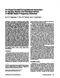
Figure 3.2: Power curve of the CAT for two-sided alternative (with n = 29 and α = 0.05) plotted against δ. C. Power for testing H0 : δ = 1 vs. HA : δ > 1 at α = 0.05. With slight modification of the steps in above (B) one can compute the power of the CAT for one sided alternative. In a comprehensive paper on testing the shape parameter of


25

a gamma distribution, Keating, Glaser and Ketchum (1990) considered the above test for testing exponentiality (i.e., H0 ) against gamma IFR (increasing failure rate) alternative. The following Table 3.2 provides the power computations ( with standard error in brackets) which is also plotted in Figure 3.3.

Table 3.2. Power of the CAT for one-sided IFR alternative (n = 29) δ Power

1.0 0.047 (0.003)

1.2 0.175 (0.005)

1.4 0.351 (0.007)

1.6 0.570 (0.007)

1.8 0.748 (0.006)

δ Power

2.0 0.876 (0.005)

2.4 0.975 (0.002)

2.8 0.996 (0.001)

3.2 0.999 (≈ 0.0)

3.6 1.000 (≈ 0.0)

1.0 0.9 0.8

βCAT

0.7 0.6 0.5 0.4 0.3 0.2 0.1 0 1

1.5

2

2.5

3

3.5

δ

Figure 3.3: Power curve of the CAT for one-sided alternative (with n = 29 and α = 0.05) plotted against δ (≥ 1). Remark 3.1 As a demonstration Keating, Glaser and Ketchum (1990) computed the power of their test procedure for the above mentioned one-sided alternative at δ = 1.59. The

26

Nabendu Pal et al.

power of their test, which depends on complicated approximate sampling distribution, turns out to be 0.56. On the other hand, the power of our proposed CAT, through simulation, at δ = 1.59 comes out to be 0.58 (with a standard error of 0.005), implying that the proposed CAT is doing as good as the previously report test, if not better. The simulation for power at δ = 1.59 has been refined with M = N = 10, 000 to make it more precise. Again, the main advantage of the CAT is that it doesn’t require the knowledge of any complicated sampling distribution, and it can be implemented through a series of computational steps. (D). 95% Two-sided Confidence Interval for δ Step-1 (i) Consider δ = 0.25, 0.5, 0.75, . . . , 2.00. Refer these as δ01 , δ02 , . . . , δ0k (where k = 8). (ii) Pretend to test H0j : δ = δ0j vs. HAj : δ 6= δ0j , 1 ≤ j ≤ k. Obtain (δˆLj , δÛj ), 1 ≤ j ≤ k, as given in the Table 3.1. These are the lower and upper critical values, and are very much data specific. Table 3.3. Lower and Upper Cut-off Points for H0 : δ = δ0 δ0 δˆL δÛ

0.25 0.175 0.395

0.50 0.348 0.833

0.75 0.517 1.265

1.00 0.685 1.727

1.25 0.863 2.184

1.50 1.020 2.702

1.75 1.188 3.181

2.00 1.338 3.655

Step-2 Plot δˆL and δÛ values against δ0 (or rather plot each pair (δˆLj , δÛj ) against δ = δ0j , 1 ≤ j ≤ k). This is given in Figure 3.4. Step-3 Draw the horizontal line at δˆL = δÛ = δˆM L = 1.67. The values of δˆL and δÛ intersected by the horizontal line provide a 95% confidence interval for δ. It turns out that the confidence interval is (0.88, 2.56). Remark 3.2 One can perform a hypothesis testing and subsequent interval estimation for the scale parameter β. The steps are similar to those for the shape parameter δ. 3.2

Weibull Distribution

A random variable X is said to have a Weibull(δ, β) (or W (δ, β)) distribution with shape parameter δ and scale parameter β provided the pdf is given as f (x | δ, β) = (δ/β δ )xδ−1 exp(−(x/β)δ ), x > 0;

(3.1)


27

10

8 δbU ≈ gU (δ0 )

bL and δbU δ

6

4 δbL ≈ gL (δ0 ) 2 δbML

0 0

1

2

3

4

5

δ0

Figure 3.4: Plot of δˆL and δÛ against δ0 for the Data Set in Example 3.1

where θ = (δ, β) ∈ Θ = R+ × R+ . The ML estimators of δ and β are found by solving the following two equations: δˆM L =

·µ X n

ˆ

XiδM L lnXi

¶Áµ X n

ı=1

ˆ

XiδM L

¶ −

i=1

and

µX n

¶ ¸−1 lnXi /n ;

i=1

µ ¶δˆM L µ X ¶ n ˆ βˆM L = XiδM L /n.

(3.2)

i=1

Example 3.2. Lieblein and Zelen (1956) gave the results of test of endurance, in millions of revolutions (m.o.r.), of 23 ball bearings with the following ordered (row-wise) observations:

17.88 51.84 68.88 128.04

28.92 51.96 84.12 173.40

33.00 54.12 93.12

41.52 55.56 98.64

42.12 67.80 105.12

45.60 68.63 105.84

48.48 68.64 127.92

28

Nabendu Pal et al.

The following histogram (Figure 3.3) is drawn with the above data set along with a matching Weibull pdf . 0.014

0.012

f (x | δ, β)

0.01

0.008

0.006

0.004

0.002

0 17.5

48.8

79.9

111.1

142.3

173.5

x

Figure 3.5: Histogram of the Endurance Data and a Matching W (δ, β) pdf with δ = 2.10204 and β = 81.8779 A formal goodness of fit test based on Coles’ (1989) methods makes a two parameter Weibull model plausible for the data set in the above example. (Details of the goodness of fit tests are omitted here.) As a demonstration of our CAT, we test H0 : δ = 1 against HA : δ 6= 1, followed by interval estimation. Again, δ = 1 reduces the Weibull distribution to a much convenient exponential distribution. (A). Test H0 : δ = 1 vs. HA : δ 6= 1 at α = 0.05 Step-1 Obtain δˆM L = 2.10204 and βˆM L = 81.8779 (from (3.2))


29

Step-2 (i) Set δ = 1 (H0 value of δ), and then find the restricted MLE of β as βˆRM L = 72.22391. (l) (ii) Now generate (X1(l) , . . . , X23 ) iid from W (1, 72.22391), 1 ≤ l ≤ M = 2, 400. For each replication obtain the MLEs of δ and β, and then retain only the δˆM L values denoted as δˆ01 , δˆ02 , . . . , δˆ0M .

(iii) The ordered replicated MLE values are δˆ0(1) ≤ δˆ0(2) ≤ · · · ≤ δˆ0(M ) . Using the 5% level of significance the lower and the upper cut-off points are obtained respectively as δˆL = δˆ0(60) = 0.7628 and δÛ = δˆ0(2340) = 1.4847. Step-3 Since δˆM L = 2.10204 is outside the interval (0.7628, 1.4847), at 5% level we reject H0 and accept HA ; i.e., the Weibull model can’t be reduced to an exponential model by taking δ = 1 for the above-mentioned data set.

(B). Power for testing H0 : δ = 1 vs. HA : δ 6= 1 at α = 0.05. The power of the proposed CAT is computed through the steps similar to those in the gamma case (using N = 5, 000) and this is presented in Table 3.4. The Figure 3.6 shows the power curve of our CAT.

Table 3.4. Power of the CAT for two sided alternative (n = 23) δ 0.2 0.4 0.6 0.8 1.0 1.2 Power 1.000 0.999 0.867 0.313 0.048 0.159 (≈ 0.0) (≈ 0.0) (0.005) (0.007) (0.003) (0.005) δ Power

1.4 0.443 (0.007)

1.6 0.746 (0.006)

1.8 0.926 (0.004)

2.0 0.984 (0.002)

3.0 1.000 (≈ 0.0)

4.0 1.000 (≈ 0.0)

Remark 3.3 For the Weibull case we have used a lower value of M to save computational time. Note that obtaining the MLEs for the Weibull distribution is much more time consuming than that for the gamma distribution.

(C). 95% Two-sided Confidence Interval for δ Step-1

(i) Consider δ = 1.0, 1.5, 2.0, . . . , 5.0; and refer these as δ0j , 1 ≤ j ≤ k (with k = 9)

30

Nabendu Pal et al.

1.0 0.9 0.8

βCAT

0.7 0.6 0.5 0.4 0.3 0.2 0.1 0 0

0.5

1

1.5

2

2.5

δ

Figure 3.6: Power curve of the CAT for two-sided alternative (with n = 23 and α = 0.05) plotted against δ.

(ii) Pretend to test H0j : δ = δ0j against HAj : δ 6= δ0j , 1 ≤ j ≤ k. Obtain (δˆLj , δÛj ), 1 ≤ j ≤ k, as mentioned in the hypothesis testing earlier. The bounds, which are very much data-dependent, are given in Table 3.5.


31

Table 3.5. Lower and Upper Cut-off Points for H0 : δ = δ0

δˆL δÛ

1.0 0.764 1.486

1.5 1.145 2.237

2.0 1.524 3.004

δ0 3.0 2.287 4.449

2.5 1.911 3.695

3.5 2.681 5.195

4.0 3.091 5.980

4.5 3.437 6.778

5.0 3.820 7.426

Step-2 δˆL and δÛ are now plotted against δ0 giving rise to a 95% confidence band for δ. This is given in Figure 3.7. 8

7

) (δ 0 gU

6

bδ U

≈

bL and δbU δ

5

4

3

bδL ≈ g L

δbML

(δ 0)

2

1

0 0

1

2

3

4

5

δ0

Figure 3.7: Plot of δˆL and δÛ against δ0 for the Data Set in Example 3.2

Step-3 The confidence interval band is intersected by the horizontal line δˆL = δÛ = δˆM L = 2.10204 gives a 95% confidence interval for α. Here, our confidence interval is (1.37, 2.86).

4

Applications to Discrete Distributions: Two Examples

The computational approach discussed earlier is now applied to two discrete distributions as demonstration. In the first example, we consider the binomial distribution, and test

32

Nabendu Pal et al.

a hypothesis on the probability of success. The power function of our CAT is then compared with the asymptotic normal test (z-test). The second example deals with the Poisson distribution, and again the power function of our CAT has been computed for a specific data set and then compared with the traditional Poisson test power. This is to demonstrate that our proposed CAT can be applied mechanically without going through the analytical derivation of the relevant test. 4.1

Binomial Distribution

Example 4.1 A box is filled with certain number of red and blue marbles. Assuming that the composition of the box is unknown, it is decided to test whether the number of red marbles is same as that of blue marbles. Twenty marbles are drawn at random with replacement from the box, and fourteen red marbles are observed. Let θ represent the proportion of red marbles in the box. The minimal sufficient statistic X, the total number of red marbles observed in 20 draws, follows B(20, θ) distribution. The MLE of θ is θˆM L = X/20 = 14/20 = 0.7. We now proceed to test H0 : θ = 0.5 vs. H0 : θ 6= 0.5 at level α = 0.05 with the observation X = 14. The usual z-test uses the approximate distribution of θˆM L , under H0 , which is N (θ0 , θ0 (1 − θ0 )/n), θ0 being the value of θ under H0 . So, for testing a general null hypothesis HA n: θ 6= θ0 , reject H0 if X is either 0 against the alternative n H0 : θ = θp o o greater p than (nθ0 ) + z(α/2) nθ0 (1 − θ0 ) or less than (nθ0 ) − z(α/2) nθ0 (1 − θ0 ) . Thus, the power of this z-test, denoted by βZ , is ¯ ³¯ ´ p ¯ ¯ βZ = βZ (θ) = P ¯X − nθ0 ¯ > z(α/2) nθ0 (1 − θ0 ) ¯ X ∼ B(n, θ) =

1−

b n o X B(n, θ) pmf at k

(4.1)

k=a

n o p where a = smallest integer greater than (nθ0 ) − z(α/2) nθ0 (1 − θ0 ) and b = largest n o p integer smaller than (nθ0 ) + z(α/2) nθ0 (1 − θ0 ) . For demonstration we use α = 0.05, n = 20 and X = 14, even though the exact value of X doesn’t play any role in the above βZ computation. However, we accept H0 : θ = 0.5 against HA : θ = 6 0.5 since X = 14 falls between the cut-off points 5.6173 and 14.3827. The exact size of this z-test is 0.0414, making it slightly conservative. Using the CAT given in Section 2, 20,000 observations (i.e., X values) are generated from the B(20, 0.5) distribution. For each of these replicated X-values, obtain the MLE of θ (pretending that it’s unknown), and call these as θˆ01 , θˆ02 , . . . , θˆ0M , M = 20, 000. Order these as θˆ0(1) ≤ θˆ0(2) ≤ · · · ≤ θˆ0(M ) . The cut-off points are θˆL = θˆ0 ((α/2)M ) = θˆ0(500) and θÛ = θˆ0 ((1 − α/2)M ) = θˆ0(19500) . If the observed θˆM L = 14/20 = 0.7 exceeds these bounds, then H0 is rejected; and accepted otherwise. Notice that the cut-off points θˆ0(500) and θˆ0(19500)


33

do not depend on the data X = 14. To calculate the power function of our CA, vary θ from 0.1 to 0.9 with an increment of 0.1. For each such θ, a large number of (say, N ) observations are generated from the B(20, θ)-distribution (referred to as second stage generation), and the power, denoted by βCAT , is calculated as ¡ βCAT = βCAT (θ) = proportion of second stage θˆ values exceeding ¢ θˆ0(500) or θˆ0(19500) . (4.2) The following Table 4.1 gives the power comparison of z-test and the CAT with N = 20, 000. Table 4.1. Power Functions of the Z-test and the CAT θ 0.1 0.2 0.3 0.4 0.5 0.6 0.7 0.8 0.9

βZ 0.9887 0.8042 0.4164 0.1272 0.0414 0.1272 0.4164 0.8042 0.9887

βCA 0.9894 0.8016 0.4124 0.1289 0.0418 0.1317 0.4107 0.8002 0.9883

Remark 4.1 (a) As expected, similar to βZ , the values of βCAT are nearly symmetric about θ = 0.5. The slight departure from symmetry (for example at θ = 0.2, βCAT = 0.8016 and at θ = 0.8, βCAT = 0.8002) is within two standard error (SE) of the simulation. The SE varied from 0.0007 to 0.0014. (b) The whole idea behind the CAT has been the assertion that not knowing or applying the sampling distribution (analytic) of θˆM L doesn’t cause much detriment as seen in Table 4.1. The βCAT -values are almost as good as the βZ -values. 4.2

Poisson Distribution

Example 4.2 The observations {4, 5, 3, 5, 5, 4} represent the number of automobile accidents per day for six randomly selected days in summer of 2005 in a particular area of a US city. Assuming that these observations are from a Poisson(θ) distribution test H0 : θ = 4 vs. HA : θ 6= 4. If we have X1 , . . . , Xn iid from Poisson (θ), then the minimal sufficient statistic X = Pn i=1 Xi ∼ P oisson(nθ). For testing H0 : θ = θ0 against HA : θ 6= θ0 , reject H0 if

34

Nabendu Pal et al.

¯ X < k1 or X > k2 where k1 < k2 are such that P (X < k1 or X > k2 ¯ θ = θ0 ) ≈ α, the level of the test. In the above data set, for testing H0 : θ = 4 against HA : θ 6= 4, we ¯ have k1 = 15 and k2 = 33 where P (X < 15 or X > 33 ¯ θ = 4) = 0.0512 (with left tail and right tail probabilities 0.019825 and 0.031382 respectively). Since for the above data, X = 26 falls between the cut-off points, we accept H0 . The power function of the above Poisson test is give by βP where βP = βP (θ) =

Pθ (X < k1 or X > k2 )

= 1 − Pθ (k1 ≤ X ≤ k2 ) h i = 1 − P oisson(θ) cdf (k2 ) − P oisson(θ) cdf (k1 ) .

(4.3)

On the other hand, we follow the CAT given in Section 2 by generating M = 20, 000 P6 observations on X = i=1 Xi from Poisson(24) and following the steps described earlier. Interestingly, the critical values (cut-off points) came out to be 15 and 34 respectively. Similar to the binomial case, we have computed the power βCAT of our CAT and this has been provided in Table 4.2 along with βP . Remark 4.2 From the table it is clear that the CAT is almost as good as the traditional analytic Poisson test. For βCAT values, which are obtained through simulation, the SE varied from 0.00025 to 0.0014. Also, it appears that the CAT is marginally more conservative than the other test. Table 4.2. Power Functions of the Poisson Test and the CAT θ 1 2 3 4 5 6 7 8 9 10

βP 0.9986 0.7720 0.2086 0.0512 0.2565 0.6530 0.9088 0.9857 0.9985 0.9999

βCAT 0.9987 0.7680 0.2058 0.0395 0.1997 0.5884 0.8818 0.9778 0.9980 0.9997

Concluding Remark: The whole idea behind this work has been to show that with the availability of cheap and fast computing facilities, statistical inference can be done solely based on computations and simulation without going through the complicated analytic


35

derivations of the sampling distributions. The computational approach (CA) adopted in this work clearly shows that, at least for the examples used here, no significant compromise has been made in terms of level or size as far as testing is concerned. As a result, applied researchers can adopt the CA without getting involved into analytical complexities.

References [1] G. Casella and E. I. George, (1992). Explaining the Gibbs sampler, The American Statistician, 46, 167–174. [2] S. G. Coles, (1989). On Goodness-of-Fit Tests for the Two-Parameter Weibull Distribution Derived from the Stabilized Probability Plot, Biometrika, 76(3), 593–598. [3] R. C. Dahiya and J. Gurland, (1972). Goodness of Fit Test for the Gamma and Exponential Distributions, Technometrics, 14, 791–801. [4] B. Efron, (1982). The Jackknife, the Bootstrap, and other Resampling Plans. CBMS 38, SIAM-NSF. [5] J. P. Keating, R. E. Glaser, and N. S. Ketchum, (1990). Testing Hypotheses about the Shape Parameter of a Gamma Distribution, Technometrcs, 32, 1, 67–82. [6] J. Lieblein and M. Zelen, (1956). Statistical Investigation of the Fatigue Life of Deep-Grove Ball Bearings, Journal of Research National Bureau of Standards, 47, 273–316. [7] F Proschan, (1963). Theoretical explanation of Observed Decreasing Failure Rate, Technometrics, 5, 375–383.