3.1.1 Linear Elements for Second-Order Equation. " 38. 3.1.2 Local ..... the penalty method; linear triangular and bilinear rectangular Stokes elements are derived ...... k (~:~ + ~:~) = f in the region nwith bound ary conditions as shown in Fig. 1.2.
Prem K. Kythe Dongming Wei
An Introduction to Linear and Nonlinear Finite Element Analysis A Computational Approach
With 152 illustrations
Springer Science+Business Media, LLC
Prem K. Kythe Department of Mathematics University of New Orleans New Orleans, LA 70148-0001 U.S.A.
Dongming Wei Department of Mathematics University of New Orleans New Orleans, LA 70148-0001 U.S.A.
Library of Congress Cataloging-in-Publication Data Kythe, Prem K. An introduction to linear and nonlinear finite element analysis : a computational approach Iby Prem K. Kythe, Dongming Wei. p. cm. Inc\udes bibliographical references and index. ISBN 978-1-4612-6466-8 ISBN 978-0-8176-8160-9 (eBook) DOI 10.1007/978-0-8176-8160-9 1. Structural analysis (Engineering) 2. Finite element method. 1. Wei, Dongming, 1958II. Title TA646.K98 2003 620'.0042- xo) square matrix unit vector in the x direction that is if and only if moment of inert ia functional ; total energy of an elastic mechanical system modified Bessel function of the first kind and order m integral defined in Example 5.2 unit vector in the y direction current Jacobian matrix thermal conductivity; permeability coefficient (aquifer)
NOTATION
kx ,ky k k(e)
K K(e)
K
Kb
l(w)
l( e)
i.i« :
L i:
c:' L M
Mo, ML M M(e)
n n n·\?
NE NL P psi P
thermal conductivity in the x and y direction unit vector in the z direction value of k on an element e constant value of a metal property; consistency coefficient stiffness matrix of an element n(e) global stiffness matrix matrix linear functional length of the interval [xie) , x~e)J length of nonuniformone-dimensional consecutive elements length of an interval; length unit; linear operator Lagrange function; Laplace transform inverseof Laplace transform matrix bending moment; polar moment of a cross-sectional area bending moment at x = a and x = L, respectively matrix matrix (radially symmetric element) power-law index outward normal vector direction cosines of n
= nx
a a a ax + n y oy + n z oz
number of elements number of local nodes on an element . I au pressure; penmeter; a so = U x = ax
Pi
lbs/irr' vertical point load; vector Legendre polynomials of degree n search direction
q
heat source; also =
qn
heat flux rate of heat generation temperature gradient shear force bending moment shear force at node i of an element n( e) vector of secondary degrees of freedom (boundary terms) part of F corresponding to the natural boundary conditions vector radial distance scalar residual (error) in the Galerkin method cylindrical polar coordinates
Pn(X)
q q
Ql Q2 Q~ e) Q(e)
Q
Qb
r
r(u) (r,e ,z)
uy =
au oy
xix
xx
NOTAT I ON
R
Rn
R+
Rj
Re ~ R(e)
R 8
(8, t) sym s(e)
t
ix ,iy
T
t;
Too
T
T( e) U
Uo Uoo
(e)
Ui
(e )
Ua U
U U
u( e)
u ,v
ii , V
Uo Ue
u (e)
U Vr
V
av
v W Wi
Wl ,W2 ,W3
W
radius Euclidean n-space set of positive real numbers errors (j = 1, . . . , n + 1) Reynolds number real part residual or error vector global error vector variable of the Laplace transform; arc length ; second(s) (time) nondimensional coordinates on the unit square symmetric (matrix) square matrix time prescribed secondary variables temperature, temperature distr ibution base temperature of a fin amb ient temperature temperature vector temperature vector for an element n( e) dependent variable; stress function; displacement; mean velocity prescribed velocit y free stream velocity value of U at node i linear interpolation function for the interval [x ~e) , x~e) ] velocity vector, displacement vector vector of the first time derivatives of u vector of the second time derivatives of u approximation of u on an element n (e) velocity components of u or v , in x and y direction approximate solution for u or v inlet velocity nodal value of U at a global node e, e = 1, . . . , NE (e)
(e)
(e)
(e)]
coIumn vector [u 1 ... uN vI .. . V N vector of global values of displacement U radial component of velocity v three-dimensional solid or volume boundary surface of a solid V velocity vector test function weights in Gaussian quadrature three different test functions work global coordinate end points of a line element
xxi
NOTATION
local coordinate ( =
a
fJ fJPY
,fJr
s
r
f 1,f z b bi j
D.t
x - x~e» )
initial guess (Newton 's method) set of nonnegative integers thermal capacitance film coefficient, convective heat transfer coefficient Dai-Yuan parameter Hestenes-Stiefel parameter specific heat ration (= cp / c,J boundary of a domain (= a n) disjoint portions of boundary I' (f 1 U f z = tolerance Kronecker delta (= 1 if i = j ; -1 if i =1= j) time step emissivity strain ; penalty parameter strain vector shear strain
an)
e
strain ( = -
{)
nondimensional temperature
~ ~, 'TJ ~i
6 ,6,6 p
a aD
a
T Txy , Tyz
¢
¢~ e)
e lj>(e)
X (e)
'IjJ
w
n
n(e)
~~); angle of twist (torsion)
= lu~e) -u~~ll , i = 1, 2, .. . , N von Karman constant eigenvalue dynamic viscosity of a fluid kinematic viscosity of a fluid (= J.L / p); Poisson's ratio (elasti city) isoparametric one-dimensional coordinate, -1 ~ 1 isoparametric two-dimensional coordinates, -1 ::::: ~ , 'TJ ::::: 1 Gaussian points trilinear coordinates density stress; Stefan-Boltzmann constant uniform load stress vector shear stress average shear stresses velocity potential of a flow basis function ; interpolation shape function global shape functions for e = 1, . . . , N + 1 vector of the shape functions for an element n (e) characteristic function for the interval [x~e), x~e) ] or n (e) stream function radian frequency domain general finite element
< :::
NOTATION
xxii
In(e)1 an an(e)
o
o
I-D 2-D
3-D \l
area or volume of an element n(e) boundary of the domain n boundary of an element n(e) null vector matrix of differential operators one-dimensional two-dimensional three-dimensional
.8 8x
.8 8y norm of a vector x
gra d =1-+J-+
k 8 8z
I x] II\lull
norm of gradient vector
\If
gradient matrix of f
\lp
pressure gra dlent
\l·F
divergence of a vector F (div F)
\l2
Laplacian
AlB
.
(8P.
a2
(
(= Jui + u~ + u~ )
= 8x 2
Bp,
8x 1 + 8yJ a
2
P
+ 88z k)
a
2
+ 8 y 2 + 8z 2
set A minus set B apprimately equal to empty set
)
An Introduction to Linear and Nonlinear Finite Element Analysis
1 Introduction
In this chapter, after a brief historical sketch about the development of the finite element methods, we discuss the weak variational formulation and present the Galerkin and Rayleigh-Ritz methods, which belong to the class of weighted residual methods . Some useful integration formulas are given in Appendix A, and Green's identities are presented in Appendix E.
1.1. Historical Sketch The pioneers in the development of the finite element method are Courant (1943), Prager and Synge (1947), Schoenberg (1948), P6lya (1952, 1954), Hersch (1955), and Weinberger (1956). Courant's work on the torsion problem is considered a classic; it defined piecewise linear polynomials over a triangulated region . Prager and Synge found approximate solutions for plane elasticity problems based on the concept of function space. Schoenberg also developed the theory of splines and used piecewise polynomials (interpolation functions) for approximation. Schoenberg also developed formulas for analytical approximation. P6lya, Hersch, and Weinberger used a technique similar to that of Courant and the finite difference methods to solve eigenvalue problems . Synge (1952) used a piecewise linear function defined on a triangulated region and the Ritz variational method to solve plane problems . Greenstadt (1959) used a discretization technique to divide the doma in into "cells," assigned a different function to each cell, and applied the variational principle . White (1962) solved a plane thermoelasticity problem, and Friedrichs (1962) developed finite difference schemes for the Dirichlet and Neumann problems. Both of them used triangular elements and the variational principle. In
P. K. Kythe et al., An Introduction to Linear and Nonlinear Finite Element Analysis © Springer Science+Business Media New York 2004
1. INTRODUCTION
2
mathematical physics, Synge (1957) developed the hypercircle method in which he provided a geometric interpretation for the minimum principle in plane elasticity. A three -dimensional electrostatic problem was for the first time solved by McMahon (1953) by using tetrahedral elements and linear interpolation functions . The name "finite element method" was first used by Clough (1960). It was shown by Melosh (1963), Jones (1964) , and de Veubeke (1964) that the finite element method can be regarded as the Ritz variational method using piecewise interpolation functions. The work of Zienkiewicw and Cheung (1965) extended the scope of the finite element method to all types of problems that could be expressed in variational form. Thus , the mid-1960s marked a transition from the early research into the modern development of the subject. From mid-1960s through 1980 this method developed from the earlier field of structural analysis into various other fields, with more mathematical analysis and different computational methods and codes. The development of mathematical theories provided a rigorous and firm foundation for the finite element methods, their Galerkin or Ritz-based variational techniques, questions of convergence, and error analysis. During this period Whiteman (1975) published a bibliography for finite elements, and Clough (1980) published an account of the development of this subject during the past 25 years.
1.2. Euler-Lagrange Equations Let H" denote the n-dimensional Euclidean space, and Z+ the set of nonnegative integers. A brief definition of functionals and the classification of boundary conditions is given below before we discuss the weak variational formulation of boundary value problems. 1.2.1. Functionals. A functional is an expression of the form
I(u) =
fin
F (x ,y,u,ux ,Uy ) dxdy+
i2
G(x ,y,u)ds,
n E R2 ,
(1.1)
where F (x, y, u , u x, u y ) and G(x , y, u) are known functions, and f 2 is a part or all of the boundary of the domain Similar functionals can be defined in R" with one or several variables . Although the value I (u) depends on u, yet for a given u, the value of I(u) is a scalar quantity. The functional I(u) represents a function defined by integrals whose arguments are themselves functions. In fact, this functional is an operator I which maps u into a scalar value I(u) . Its domain is the set of all functions u(x), whereas its range, which is a subset of the real field, is the set of images of all functions u under the map I . Frequently the functional I (u) represents the total potential energy of a mechanical system and a stationary point of I is sought to satisfy the equation
an
n.
d dT I(u
+ TV)
= 0
(1.2)
1.3. WEAK VARIATIONAL FORM
3
for all real numbers T and all v such that u + TV is admissible for I. The set of admissible functions is defined to be those functions on n that give finite values of I(u) and satisfy the condition r1 = fL, where 1 is the boundary ofn minus z . As a result of the calculations of the values ofEq (1.2), we obtain the corresponding Euler-Lagrange equation
ul
of
OU -
r
0 (OF) 0 (OF)
ox op - oy oq = 0
r
inn,
(1.3)
subject to the boundary conditions
(1.4a) (lAb) where F = F(x, y, u, p, q), p = u x , q = u y , and n x , n y are the direction cosines of the unit vector n normal to the boundary on := I' = I' 1ur z of a two-dimensional region n such that r 1 n r z = 0. For details, see Axelsson and Barker (1984) .
1.2.2. Boundary Conditions. A partial differential equation is subject to certain conditions in the form of initial or boundary conditions. The initial conditions, also known as Cauchy conditions, are the values of the unknown function u and an appropriate number of its derivatives at the initial point. The homogeneous boundary conditions fall into the following three categories: (i) Dirichlet boundary conditions (also known as boundary conditions ofthe first kind, or essential boundary conditions), when values of the unknown function u are prescribed at each point of the boundary r 1 of a given domain n. (ii) Neumann boundary conditions (also known as boundary conditions of the
second kind), when the values of the normal derivatives of the unknown function
u are prescribed at each point of the boundary r z.
(iii) Robin boundary conditions (also known as boundary conditions of the third kind, or mixed boundary conditions), when the values of a linear combination of the unknown function u and its normal derivative are prescribed at each point of the boundary r z. The last two conditions are also known as the natural boundary conditions.
1.3. Weak Variational Form The weak variation formulation of boundary value problems is derived from the fact that variational methods for finding approximate solutions of boundary value problems, viz., Galerkin, Rayleigh-Ritz, collocation, or other weighted residual
1. INTRODUCTION
4
methods, are based on the weak variational statements of the boundary value problems. For example, a special case of (1.3) is when F is defined as
F
8u ) 2 2 ( 8u ) 2] ="21 [ k1 ( 8x + k 8y
- I u.
This equation arises in heat conduction problems in a two-dimensional region with k1 , k2 as thermal conductivities in the x , y directions, and I being the heat source (or sink) . Here
8F 8u = -I,
8F _ k 8u 8p - 18x' and Eq (1.3) becomes
-:x (k ~~) :y (k ~~) 1
2
-
=
I
In
If k 1 = k2 = 1, then we get the Poisson's equation - 'V2 u =
n.
(1.5)
I
with appropriate
boundary conditions. The weak variational formulation for the boundary value problem (1.3)-(1.4) is obtained by the following three steps . STEP 1. Multiply Eq (1.3) by a test function wand integrate the product over
the region
n:
_ ~ (8F)] w dxdy jJr [8F8u _ ~8x (8F) 8p 8y Bq e
0.
= O.
(1.6)
The test function w is arbitrary, but it must satisfy the homogeneous essential boundary conditions (1.4a) on u. STEP 2 . Use formula (A.8) componentwise to the second and third terms in (1.6) for transferring the differentiation from the dependent variable u to the test function w, and identify the type of the boundary conditions admissible by the variational form:
8w8F 8W8F] r (8F 8F) j"rJn [8F rt: + 8x 8p + 8y 8q dxdy- Jan x>: x> wds=O.
(1.7) Note that formula (A.8) does not apply to the first term in the integrand in (1.6) . This step also yields boundary terms that determine the nature of the essential and natural boundary conditions for the problem . The general rule to identify the essential and natural boundary conditions for (1.3) is as follows . The essential boundary condition is prescribed on the dependent variable (u in this case), i.e.,
u=
u
on
f
1
5
1.3. WEAK VARIATIONAL FORM
is the essential boundary condition for (1.3). The test function w in the boundary integral (1.7) satisfies the homogeneous form of the same boundary condition as that prescribed on u. The natural boundary condition arises by specifying the coefficients of wand its derivatives in the boundary integral in (1.7). Thus,
8F 8p n x
8F
8G
+ 8q n y + 8u = 0
on
I' 2
is the natural boundary condition in a Neumann boundary value problem. In onedimensional problems, use integration by parts instead of formula (A.8) . To equalize the continuity requirements on u and w, the differentiation in formula (A.8) is transferred from F to w. It imparts weaker continuity requirements on the solution u in the variational problem than in the original equation. STEP 3 . Simplify the boundary terms by using the prescribed boundary conditions. This affects the boundary integral in (1.7), which is split into two terms, one on I' I and the other on I' 2 :
Jinr r
[8F w 8u
8w 8F
8w 8F]
J
(8F
8F
)
+ ax 8p + ay aq dx dy- ! f'tUf' 2 ap n x + auyn y w ds =
O.
(1.8)
The integral on f l vanishes since w = 0 on fl . The natural boundary condition is substituted in the integral on f 2 . Then (1.8) reduces to
r [aF aw 8F 8w 8F] r ec w au + 8x 8p + ay 8q dx dy + if'2W 8u ds = O.
J
in r
(1.9)
This is the weak variational form for the problem (1.3). We can write Eq (1.9) in terms of the bilinear and linear differential forms as
b(w, u) = l(w) , where
(1.10)
=Jrrin [8W8F + 8W8F] dxdy, 8x 8p 8y 8q 8F 8G l(w) = _Jrr w dxdy- r w ds. in 8u i r 8u
b(w,u)
(1.11)
2
Formula (1.1 0) defines the weak variational form for Eq (1.3) subject to the boundary conditions (1.4) . The quadratic functional associated with this variational form is given by
1 I(u) = "2b(u , u) -l(u).
(1.12)
EXAMPLE 1.1 . Derive the Euler-Lagrange equation and the natural boundary condition for the functional
I(u)
=
l
a
b
"21 [p(x)(u) 2 + q(x) u 2 - r(x) u] dx + "21 ap(a) [u(a)]2 , u EU, I
(1.13)
1. INTRODUCTION
6
where U = {u E C 2 [a, b], u(b) = B} . We write the functional (1. 13) as
l
I (u) = Let
g(T) = Now, since
dg(T)
d dT
~ =
l
b
I
b
=
I
a
o(u
a
b
a
[
F (x ,u, u x ) dx + C(a,u(a)) .
(1.14)
F (x, u + TTJ ,Ux + TTJx) dx + C(a , u(a) + TTJ(a)) .
b[
=l
b
F (x , u + TTJ ,Ux + TTJx) dx
d
+ dTC (a, u(a) + TTJ(a))
d(U+TTJ )+ of d(UX+T TJx )] dx dr o(u x + TTJx) dr + ---,----,-O_C_.,.......,...., d(U(a) + TTJ (a)) o(u(a) + TTJ(a)) dr
of
+ TTJ)
OF 1] + OF OC TJx] dx + TJ (a), o(u + TTJ ) o(u x + TTJx) ou(a) + TTJ (a)
(1.15)
we find that
dg(O )
~
=
I
b
a
[OF OF] OC au 1] + oUx 1]x dx + ou(a) TJ(a) = O.
Thus, after integration by parts we get
or
I
a
b
[OF OF)] TJdx+~ o f I TJ(b) -~ of I TJ(a)+~ oc( ) TJ (a) = O. ~ - !al ( ~ uU ox uux uux x=b uux x=a uU a (1.16)
Now, for U+TTJ to be inU, we have u(b) B ; thus, TTJ (b ) = 0, or TJ (b ) = O. Then
dg(O) -= dr
I
a
b
= B, U(b)+TTJ(b) = B, i.e., B+TTJ(b)
[OF - - -a ( -OF)] n dx au ax OU x
>
-
of I TJ (a) + ec- TJ (a) = o. oUx x=a o(u(a)
(1.17)
= TJ(b) = 0, the equation
For all TJ satisfying TJ(a)
I
a
b
[OF au
_~( OF)] ax oU x
=
TJ dx=O
1.3. WEAK VARIATIONAL FORM
7
implies that -8F - -8 (8F) - - -_ 0
8u
in (a,b),
8x 8u x
if it is continuous in (a, b) . Also,
- -88FI U
8G
( ) 1](a) = x x=a1](a) + -U8 a
0 for all1](a)
implies that
:~ Ix=a
8G
8u(a)'
Then the Euler-Lagrange equation is
~~ - ~ (:~) = 0
in (a,b).
(1.18)
Further, since
8F
and 8u
[p( x) (ux)2 +q(x)u 2 - r (x ) u],
F(x ,u,ux ) =
~
G(a,u(a))
"2o: p(a) [u(a)] ,
=
1
2
8F
8G
= q(x) u - r(x), 8u = p(x) ux , and 8u(a) = o:p(a) u(a), the Eulerx
Lagrange equation (1.1 8) reduces to
d [p(x) dx dU] = 0, q(x) u - r(x) - dx
(1.19)
subject to the natural condition
8F I -8
U x x=a
Finally, since U x Ix=a -
= p(x) Ux I
0:
x =a
u(a)
= -8G 8 ( ) = o: p(a)u(a). U
a
= 0, the Euler-Lagrange equation (1.19) becomes
d [p(x) dx dU] = 0, q(x) u - r(x) - dx subject to the natural condition
dul -d X
x =a
= o:u(a).•
In the next example we derive the bilinear and linear forms for a system of partial differential equations in two variables with prescribed boundary conditions.
1. INTRODUCTION
8
1.2 . Consider the system of Navier-Stokes equations for a twodimensional flow of a viscous, incompressible fluid (pressure-velocity fields): EXAMPLE
ou + vou = _~ op + v (02 u2 + 02 U ) oX oy Pox ox oy2 ' OV ov lop (02 v 02 v) U ox + voy = - poy + u ox2 + oy2 ' OU ov ox + oy = 0,
U
in a region
n, with boundary conditions u = Uo, v = Vo on f l , and Ou) OU ox n x + oy n y ov ov) v ( ox n x + oy n y
v (
-
p1 pn x = t,« .
-
p1 pn y = t,y ,
on I' 2, where (U ,v) denotes the velocity field, p the pressure, and ix ,i y the prescribed values ofthe secondary variables. Let WI, W2, W 3 be the test functions, one for each equation, such that WI and W2 satisfy the essential boundary conditions on U and v, respectively, and W3 does not satisfy any essential condition. Then
1.4. GALERKIN METHOD
9
Note that the boundary integral in the linear form l (WI , W2, W3) has no term containing W3 . •
1.4. Galerkin Method We discuss two frequently used methods for obtaining approximate numerical solutions of boundary value problems. They are Galerkin and Rayleigh-Ritz methods. These methods give the same results for homogeneous boundary value problems. Consider the boundary value problem
Lu=f
inn,
(1.20)
on I'i .
(1.21 )
subject to the boundary conditions
u=g au an + ku
on f
h
=
(1.22)
2,
where I' = I'j U I' 2 is the boundary of the region n . Let us choose an approximate solution u of the form N
U=
:L Ui i Ii = fin 4>d !1
J::)
uX
84>j J::)
uX
J::)
UY
84>j) dx dY, J::)
UY
Now, if we choose Ui such that J(Ui) is a minimum (i.e., 8J/ 8Ui (1.30) we get
L KijUi = j=1
Ii,
i = 1, ' "
(1.31 )
(1.32)
dxdy.
n
(1.30)
,n,
= 0), then from (1.33)
1.5. RAYLEIGH-RITZ METHOD
13
which in the matrix notation is
Ku=f,
(1.34)
where the matrix K has elements K ij given by (1.31), the vector f has elements
I. given by (1.32), and the vector u = [U1' . .. ,un]T. Note that (1.34) is a system
of linear algebraic equations to be solved for the unknown parameter Ui , and K is nonsingular if L is positive definite.
The Rayleigh-Ritz method is alternatively developed by solving the equation (1.10) for u, where we require that w satisfy the homogeneous essential conditions only. Then this problem is equivalent to minimizing the functional (1.12) . In other words , we will find an approximate solution of (1.10) in the form n
Un = L UjrPj + rPo, j=l
(1.35 )
where the functions rPj, j = 1, .. . ,n, satisfy the homogeneous boundary conditions while the function rPo satisfies the nonhomogeneous boundary condition , and the coefficients Uj are chosen such that Eq (1.10) is true for w = rPi, i = 1, . . . ,n, i.e., b(rPi' un) = l(rPi), or for i = 1"" ,n,
Thus, n
LUjb(rPi,rPj) = l(rPi) - b(rPi, rPO) , j=l
i
= 1, , "
,no
(1.36)
This is a system of n linear algebraic equations in n unknowns Uj and has a uniqu e solution if the coefficient matrix in (1.36) is nonsingular and thus has an inverse. The functions rPi must satisfy the following requirements: (i) rPi be well defined such that b(rPi, rPj ) =I- 0, (ii) rPi satisfy at least the essential homogeneous boundary condition, (iii) the set {rPi}i=l be linearly independent, and (iv) the set {rPd i=l be complete. The term rPo in the representation (1.35) is dropped if all boundary conditions are homogeneous. EXAMPLE 1.5 . Consider the Bessel's equation X
Set U = v
+ x.
2
U"
+ xu' + (x 2 -
l)u = 0,
u(l) = 1, u(2) = 2.
Then the given equation and the boundary conditions become
211 X V
+ xv / + (x 2 - l)v + x 3 = 0, v(l) =
°= v (2).
1. INTRODUCTION
14
In the self-adjoint form this equation is written as x 2 -1
+ v' + - - v + x 2 = O.
xv"
X
For the first approximation, we take
= al¢1 = al(x -1)(x -
VI
2).
Then using (1.25) we get f12(LvI - J)¢I dx = 0, which gives
JIr [2a Ix 2
(3 - 2x)al
2
x 1 + ~(x -
1)(x - 2)al + x 2] (x - 1)(x - 2) dx= 0,
which, on integration, yields al = -0.811, and thus, UI
= VI
+X =
-0.811(x - 1)(x - 2) + x.
Theexactsolutionisu = CI J I(X)+C2 YI(X), where c, = 3.60756, C2 = 0.75229. A comparison with the exact solution in the following table shows that UI is a good approximation. Table 1.1.
EXAMPLE
x
UI
1.3 1.5 1.8
1.4703 1.7027 1.9297
Uexact
1.4706 1.7026 1.9294.
1.6. Consider the fourth-order equation
[(x + 2l)u"]" + bu - kx
= 0,
0
< x < l,
with the boundary conditions: u(l) = 0 = u'(l), (x 2l)u"]' (0) = O. We choose the test functions
+ 2l)u"(0) = 0,
¢I(X)
=
(x _l)2(x 2 + 2lx + 3l2) ,
(h(x)
=
(x -l)3(3x 2
For the first approximation, we have UI 0, which gives
[(x +
+ 4lx + 3z2).
= al¢1 (x) . Then f~ (LUI - J)¢I (x) dx =
15
1.5. RAYLEIGH-RIT Z METH OD
If, for example, we take I
= 1=
band k
= 3, then a1 = 0.0119174, and thus ,
U1 = 0.0119174 (x - 1)2(x 2 + 2x
For the second approx imation, we take U2 = a1 0, f
= const,
where EI is called the flexural rigidity of the beam, subject to the boundary conditions
du u(O) = 0 = dx (0) ,
d2UI E I -2 = M o, dX x= L
.!!dx (El dx 2 ) Ix =L = d2U
0.
1.6. EXERCISES
21
r
L
ANS.
d2w d2 u b(w,u) = Jo EI dx 2 dx 2 dx,
r wf dx + w(O) [ddx ( EI dw l(w) = - Jo dx dU)] dx
x= o
] [El du dx
dx
L
_ [dW] dx
x=o
x=o
_ fow(l) + mo [dw]
1.8. Use the Galerkin or Rayleigh-Ritz method to solve {(x, y) : 0 < x , Y < I} such that
u(l , y) by choosing (a) w (b) w
= ¢i = cos
= 0 = u(x , 1),
= ¢i = (1 -
(2i - 1)1TX 2
au
\J2 U
x= L
=
.
1 in S1 =
au
an (0, y) = 0 = an (x ,0),
x i )(l
- yi) for i = 1, . .. ,N, or (2i - 1 )1TY . cos 2 for z = 1, . . . ,N.
ANS. (a) This choice satisfies the essential boundary conditions, but not the natural boundary conditions. Hence, we assume the first approximate solution as U1 = a¢l, ¢1 = (1 - x 2)(1 - y2). The exact solution is
u(x ,y)
~{(1- y2)
=
+ 32
1T 3
f
( _l)k cos[(2k - 1)1Ty/2] cosh[(2k - 1)1Tx/2] } (2k-1) 3cosh[(2k-1)1T/2] .
k=l
The second choice can be dealt similarly . 1.9. Find the approximate solution by the Galerkin method for the nonlinear problem Ut = U x x + €U 2 on 0 < x < 1, subject to the boundary conditions u(O ,t) = = u(l,t) and the initial condition u(x ,O) = 1, by choosing ¢j(x) = sin jrrz .
° N
ANS.
L
j ,k=l
{I-Uj(t) 2
1
+ 21T where
1 1T2 Uj (t ) + _j2
L
2
€
[2(1 -
COSj1T) .
3]1T
um(t)f(m, n,j)J} , m, n
=
u;(t)
1,2 , · ·· ,N,
m#n
.) 1-cos(m-n+j)1T 1-cos(m-n-j)1T f( m,n,] = . . m-n+] m-n-] 1 - cos(m + n + j)1T 1 - cos( m + n - j)1T . + . ' m+n+] m+n-] 1
To find Uj(O), solve fo ¢j Rd x = 0, where R =
N
L j ,k= l
Uj(O) ¢j(x) - 1.
22
1. INTRODUCTION
1.10. Usethe Galerkinmethodto solvethe Poisson's equation \7zu = 2 subjectto theDirichletboundary conditionu = 0 alongtheboundaryofthesquare{-a :::; x , y :::; a} by choosing (a) the basis functions ¢(x, y) = (a 2 - x 2)(a2 _ y2), and consideringthe approximate solution
ANS. For N = 1, we have
This yields
We must have A z = A 3 . Then for N
= 3, take
where A _ 1 -
1295
A2
1416az '
=~=A 4432a4 3·
This gives U2 (X, y)
= ~2 (a2 4432a
. . (b) The baS1S functions
x 2)(a2 - y2)
[74 + a15(x 2 + y2)] . 2
j1l'X k7l'y . cos - , where), k are odd, and 2a a
= cos -
¢jk
-
L
UN =
j,k=l j ,k odd
j1l'X
k7l'y
Cl! 'kCOS- C O S - , J a 2a
which leads to
j 21l'2 k 21l' 2) [ ( afa + -4af Z L.J 4a2 -a
-a
' " Cl!'k J
--
j1l'X a
COS -
j ,k
X
Hence, for j
m1l'X k1l'y cos - - cos dxdy 2a 2a
= m and k = n , Cl!jk
k7l'Xy] 2a
COS--
128a2(_1)(j+k-2) /2 = jk(P + P)1l'4
= O.
1.6. EXERCISES
23
1.11. Use the Galerkin method to determine the lowest frequency (fundamental tone) of the vibration of a homogeneous circular plate n of radius a and center at the origin of cylindrical polar coordinates, clamped at the entire edge, i.e., solve V'4 u = AU subject to the conditions u(a) = 0 = ur(a). HINT . Change to polar coordinates, and take UN =
L (Xj ( 1 -
ANS. Solve
j=l
N
r2
a2 )
j+1 •
Then for N = 2, we have (Xl (192 _
9
4) 4) Aa + (l2 (144 _ Aa 5
4) (ll (144 _ Aa 9
+(X2
6
9
6
5
7
= 0
4) (96 _ Aa =0
'
'
and the equation for A is
(Aa4)2 _ 97;2 Aa4 + 435456 = 0, .
104.387654
which has the smaller root as A =
4
..
.
Using this value of A in the
.
a above system of two equations, we find (l2 = 0.325 (l l, and
U2 = (ll [ (1 -
:~
r
+ 0.325 ( 1 -
:~
r],
where (Xl can be found from the above system of two equations. 1.12. Use the Galerkin method to solve the boundary value problem of Example 1.3 by taking the first-order approximate solution as N
=
Ul
s:
~
k
.
. J1rX.
1ry
(Xjksm~sm-b-'
j ,k=l
which is an orthogonal trigonometric series with a finite number of terms, such that
l
a
o
m
f;
n
a/2 , m
=
n.
{ 0, . m1rX . n1rX sm--sm--dx =
a
a
SOLUTION . Note that Ul satisfies the boundary conditions. Then the Galerkin equation (l .26a) gives
fJ[ (7 b a
(Xjk
o
0
j 21r2
k 21r2 )
+~
j 1rX k1ry sin ~ sin -b-
]
jtt«
k1ry
+ c sin ~sin -b- dx dy =
O.
1. INTRODUCTION
24
Hence,
7r
(j2-
2
0: "k J 4
a2
2
C + -kb2 ) = -. -(1 )k7r 2
.
cos)7r)(1 - cos k7l"),
which yields
Thus, this approximate solution is
Note that
Ul
becomes the exact solution Uo as N
-> 00 .
At the center point
(a/2, b/2), we have
If a = b, then at the center point (a/2 ,a/2)
_",,,,4a 2c(1-cosj7r)(1- cosk7l") . j 7r . k7l" Ut ,center -
L
j
L
"kTr4( "2 J J
k
+ k2)
sin 2 sm 2
= a2c[8+~+~+~+ " '] =uo~ 36.64 c(~) 2 . 4 4 7r
15
15
81
7r
2
1.13. Let
I(u)
=
r ~ [p(x ,Y) IVuI
in 2
+
1vl
2
1
an,
r (x, y) u] dxdy 2
"2O:(x ,y)p(x,y)u ds,
r2 u E V = {v E C )n ), r l 2
+ q(x, y) u2 -
= o:(x , y)} ,
where r 1 ur 2 = r 1 nr 2 = 0. Derive the corresponding Euler-Lagrange equation and the natural boundary condition.
2 One-Dimensional Shape Functions
The Galerkin finite element method requires the use of the test functions w in polynomial form . We will first define the local and global linear and quadratic Lagrange and Hermite interpolation shape functions. These interpolation shape functions are used in the next two chapters to solve one-dimensional stead y-state second-order and fourth-order boundary value problem s by finite element method s.
2.1. Local and Global Linear Shape Functions Before we proceed with the Galerkin finite element method , we introduce some basic Lagrange finite element interpolation shape function s, which are used in solving the second-order bar (or potential) equation s. We discretize a finite interval [0, L] by dividing it into N subintervals by a partition
0=
Xl
< X2 < ... < XN < XN+ l
= L,
[xi el, x~e)], where e = a linear finite element nee) of length lee) =
and denote a typical subinterval by
1, . .. , N . This sub-
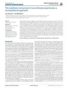
interval denotes x~e) - xi el. The end points of this subinterval are called the global nodes of the element, which are labeled e and e + 1 in bold face for e = 1, . . . , N for an N -element mesh of linear elements. For example, a 4-element mesh of the interval [0, L] is schematically presented in Fig. 2.1(a), where the global nodes are marked by 1, 2, 3, 4 (in bold) . The local nodes for each element are marked over the global nodes by 1, 2.
P. K. Kythe et al., An Introduction to Linear and Nonlinear Finite Element Analysis © Springer Science+Business Media New York 2004
26
2. ONE-DIMENSIONAL SHAPE FUN CTIONS
The point-slope form of the equation of the straight line passing through the two points (x(e) and (x 2(e), u(e» I , u(e») I 2 ) is ( Y - uI
e)
U2(e ) - U(le) ( X (e ) (e ) X 2 - Xl
=
X(le)
)
,
which can be rewritten as
where (e)
(e)
X2
¢l (X) =
(e)
X2
-
X
(2.1)
(e) '
Xl
-
are called the local linear interpolation shape fun ction s, or simply the local shape fun ction s. These shape functions are defined in the global sense (with respect to the variable X). I (e)
0
o~-- - - - tXl""1 Xl (e)
X
Global
I
1
•1
u1 1
•1
n (1)
CD
2
2•
1
•
2
e )
I
2 I
@
U2
2
rxl
@ [( e)
2. 1
CD
I
d e)
•
CD
3
u3
n (2)
2
@
3
I
• 3•
2
•
x = o u (eL u 1 - e
4
U4
1
•
n (3 )
2
CD
4
X =Xl (e)
•
x=! (e) d e)
®
u (e)= U 2 e+ l
2
•
X =x (e) 2
(b)
(a) Fig. 2.1. A Typical Finite Element Mesh Scheme. However, in the local sense, i.e., with respect to the variable ii , where x + x ~e) (see Fig. 2.1(b)), these functions become
(e) (_) _ X ¢l X -1-~,
(e)( _
o::; x < l (e ) .
X
¢2 x) =~ ,
X
=
(2.2)
Let X
E
[x(e) x (e)] , I , 2
denote this linear interpolation function for the interval [x~e) , x~e) ].
(2.3)
2.1. LOCAL AND GLOBAL LINEAR SHAPE F UNCTIONS
27
e The characteristic function associated with the interval [x i ), x~e) ] is defined by
x(e)(x)
={
x E [xie) , x~e)],
1, 0,
x
rf
'F
[x (e) x (e) ] l
'
2
(2.4)
,
for e = 1, .. . , N . The global piecewise linear interpolation function associated with the above partition 0 = Xl < X2 < .. . < XN < XN+! = L is defined by N
X E [O ,L].
ua(x ) = LX (e )(x)u~e ) (x), e= I
LetUI
( 1)
= UI
(1)
, U2 =U 2 "", UN
( N) =U 1 ,
( N)
and UN+I =u2 . Then
N N+I e i( X)Ui , ua(x) = L x(e)(x )[¢ie)(x)ui ) + ¢~e) (x) u~e)] =
L
e= I
X E [O, L],
i=l
(2.5)
where
I(X)
= X(l )(x)
¢i1) (x),
2(X) = x (l )(x ) ¢~l) (x)
+ X(2l(x) ¢i2) (x),
N(X) = x (N)(x) ¢~N- l) (x) N+!(X) = X( N)(x) ¢~N)(x),
,,
,,
+ X(N)(x) ¢iN)(x ), x E [O ,L] .
/
/
,,
/
,,
/
-,
- - - - - - -'F---------'.,:- - - - - __- - -
e-2
e
e -1
e+1
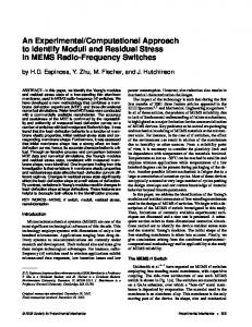
Fig. 2.2. Linear Global Shape Functions. The tent-shaped functions 1(x), . .. , N+l (x), defined on [0, L] and shown in Fig . 2.2, are called the global piecewise li near shape fun ctions associated with the partition 0 = Xl < X2 < .. . < XN < XN+! = L , or simply, the lin ear global shape functions associated with the above partition . They can be represented as
'f Xe - l ::; X ::; Xe'
d,(e -l)
'1'2
e --
d,(e)
{
'1'1
o
1
'f Xe < _ X ::; Xe+I,
1
elsewhere.
(2.6)
28
2. ONE-DIMENSIONAL SHAPE FUNCTIONS
This result will be useful in defining the function u continuously for any value of x E (0, l) in terms of the nodal values Ui, i = 1, .. . ,N.
2.2. Local and Global Quadratic Shape Functions e)
Consider a finite element n( e) that consists of the end points xi and x~e) and the midpoint with x~e) such that x~e) = xie) + l (e) /2, where l (e) = x~e) - xi e) denotes the length of the element. * The unique quadratic function of the form
+ bx + c passing
u (e)( x) = ax 2
(x~e) , u~e)), and (x~e) , u~e))
through the three given points
(x ~e), uie )),
can be determined by solving for the undetermined
coefficients a, b. and c from the following system : 1
(2.7)
1 1
We will use Cramer's rule to solve this system. For the sake of simplicity we use the following notation:
IDI=
ID2 1 =
(xie)f xl(e)
1
(x~e)f
(e ) x2
1 ,
(x~e)) 2
(e ) x3
1
(e)
(e ) UI
1
x~e)f
(e ) U2
1 ,
(x~e)f
(e) U3
1
1 1 ,
Xl
(e) x2 (e) x3
(xie)f
(x~e)) 2 (
IDI I =
(e) UI (e) u2 (e ) U3
1 Xl
(e)
(e) UI
(
x~e) f
(e) X2
(e) U2
(
x~e)f
(e) X3
(e) u3
c=
lDT'
ID3 1 =
Then a
=
IDII
lDT'
b
= ID2 1
IDI'
jD3 1
*The len gth z( e) of a n element n( e) is always the d ist ance between the two end poi nt s of the element , i.e., z( e) = x~e) - x~e) . For a n N-n od e eleme nt ( N ~ 3) , there are two end points x ~e) and x~e ) , a nd (N - 2) int erior points whi ch are den ot ed by x~e), k = 3, . . . , N . For unifo rmly spaced nod es the inter ior points ar e defined succe ssively by (e) _ (k - 2) z( e) xk for k= 3, . . . ,N. N -1
2.2. LOCA L AND GLOBAL QUADRATIC SHAPE F UNCTIONS
29
Thus, the quadratic interpolation function is given by
(2.8) Rearranging the terms, this can be written as
where 2
X
rPi ) (X) e
=
I X(e) 2 (e) x3
~1 + X(-l)
(x~e) ) 2
1
( x~e) f
1
+
(x~e)) 2 X2(e)
(x~e)f
IDI
x2
X
(x~e)) 2 x 2(e) ( x~e) f
1 1
(e) x3 1
IDI
rP~e ) (x ) =
I (e ) x 2( - 1) x te) x3 ( x ie)f X2
(x~e) f
~ I+x
(e) 1 Xl X 1 (e) x3 1
IDI 2
X rP~e) (x) =
I Xl(e) (e) x2
(e) x3
~ 1+ X(-l)
( xie)) 2 Xl(e) 1 (e) ( x~e)f x 2 1 x2 X 1
( x ie)f
1
( x~e) f
1
+ (- 1)
IDI
( xie)) 2
(x~e)f IDI
1 1
+
(x ie))2 x 2(e) (x~e)f x 3(e)
( x ie)) 2
(x~e) ) 2
(e) Xl (e) x2
IDI
These quadratic functions rPi ) (x) , rP~e) (x), and rP~e) (x) are called the local quadrati c shape func tions associa ted with the partition 0 = Xl < X2 < .. . < e
30
2. ONE-DIMENSIONAL SHAPE FUN CTIONS
XN < XN+ l = L. By evaluating the determinants, they can be also written in the following form:
(X~e) _ X) (X~e) - X) e) (X2 -
(e) ) ( X e) -
Xl
3
(e) ) ,
Xl
( x~e) _ X) (x~e) - X) (Xl
(2.9)
e) - X(e)) ( X3e) - X2(e )) , 2
(x~e) _ X) (x~e) - X) (Xl
e) - X(e) ) ( X e) - X3(e) ) . 2 3
In terms of the local coordinates ii , where
X
= x~e )
+ x, the local cubic shape
functions (2.9) reduce to _ ¢ (e) l (x) =
(
X ) (1 - ~ 2x ) , 1- ~
(e) _ _ X ( X ) ¢2 (X) - 4 ~ 1 - ~ , (e)
_
X (
(2.10)
2X)
¢3 (x ) = -~ 1 - ~ ,
= x~e) - x ~e) , and x~e) = l(e)/2. Note thatthese interpolation functions have the properties: (i) ¢~e) ( x )e)) = where l(e) denotes the length of the element, i.e., l(e) n
n
i =l
i =l
Oij, and (ii) L ¢~e) (x) = 1, which implies that L d::
(~
= O.
The graphs of
these shape functions are presented in Fig. 2.3. Similarly, we can define the corresponding global and local cubic shape functions .
-------
x
",,"---~'7----~-:---_-----':~-------,,"' ---
2
Fig. 2.3. Local Quadratic Shape Functions.
3
I
2.4. HERMITE SHAPE FUNCTIONS
31
2.3. Parametric Coordinates Consider the linear transformation
e The inverse of e(x) is x(e) = xie) + (x~e) -xie))e. Thus, we have cPi ) (x(e))
e.
and cP~e) (x(e)) = 1 coordinate. The functions
Since it is dimensionless,
=e
e is called a parametric e
are called the local linear shape functions in the parametric coordinate associated e e with cPi ) (x) and cP~e)(x). We can verify that cPi ) (x(e)) = cPI(e), cP~e) (x (e)) = e e cP2(e), and cPI(e(X)) = cPi ) (x), cP2(e(X)) = cP~e) (x) . We also have e(xi )) = 0,
e(x2e)) = 1, 0 :::; e:: ; 1, ddex dx _ ( e) de - x 2 -
=
(e)
x2
1 -
( )
(e)' X 0 xl
= Xl(e ), X() 1 =
(e) x 2 , and
(e) Xl .
Similarly, for the the three quadratic shape functions defined in §2.2, let _
x-
(e)
X3
+ Xl(e) 2
+
(X e) 3
-
2
(e) ) c
Xl
~e ) (x )u~e) and w =
¢je) (x ) that are defined in (2.1) or (2.2),
i= I
we obtain the finite element equation n
" = F)(e), L...K(e)ute) 1))
J. = 1, 2 ,. . . , n ,
i= I
where
Note that for the above linear element n (e) , we have set
EA du ( (e) ) _ _ p ee) l ' dx Xl
EA(3TI X-X _ (e) = T 1(e), l
( (e) ) _ p ee) EA du 2 , dx X2 (e) _ p ee) + T (e) Q1 - I I '
EA(3T Ix-x2 _ (e) = TJe),
(e) _ p ee) _ T (e) Q2 - 2 2 '
3.1. GALERKIN FINITE ELEMENT METHOD
Thus, for e
= 1, ...
K( c ) = _E
, NE, (c ) xl
(6 _
L(c)
F
(c ) _
(_
- (JE T 6
xi
c
)
(c) ) + X2
F (l )
3
x
[
+ x~C) ) {-1 }
0 2
1
{
-5 .5 } 5.5
3
106 [4.5 -4.5
F (2) =
216 x 102 {-4.5} 4.5
= 3 106 [3.5 x
-3.5
Hence, the assembled equation K U
[ o
o
-5.5 10.0 - 4.5
o
o -4.5 8.0 -3.5
+
1
)
}
(e)' 2
Q
l
+ 104 {5} + { Qi ) } 5
Q ~l)
'
-4.5] 4.5 ' 2
+ 104 {5} + { Qi ) } 5
Q~2 )
'
- 3.5 ] 3.5 '
F(3) = 216 x 102 {-3.5} 3.5
5.5 -5.5
2
{Qi
C
1}
l (c)L( c) {
-5.5] 5.5 '
K (2) =
K (3)
+
= 104 and L(c ) = 10, we find that
106 [5.5 -5.5
= 216 x 102
x
-1 ] 1 '
1 -1
20
For a 3-element model, with 1(0)) K (l) =
55
=F
+ 10(4)
{5} 5
3 )}
+ { Qi
Q~3)
'
becomes
0] {UI} U2 U3 U4
0 - 3.5 3.5
(3.27)
l
-0.0229333 } _ 0.0405333 - { 0.0405333 0.0418667
Qi Q~l) + Qi
{
)
2
)
+ Q~2) + Q P )
}
.
Q ~3 )
ui
) = 0 (essential), and Q~l ) + From the boundary conditions, we have UI = 2 Qi2) = 0 = Q ~2) + Qi3), and Q~l) + Q i ) = 0 = Q~2) + Qi3); also, Q~3) = p~3) _ T? ) = P - T~3) = 400 - {JE T (6 - 30/10) = - 64400, which yields (10- 6/ 3) Q~3) = -0.0214667. Thus, the system (3.27) reduces to l
5.5 -5.5 [
o o
-5.5 10.0 - 4.5
o
o -4.5 8.0 -3.5
J{UO}
00 -3.5 3.5
2
U3 U4
_
-
{-0.0229333} 0.0405333 0.0405333 0.0418667
6 l { 10+ 0 )/3 } 0 ' -0.0214667
Qi
56
3. ONE-DIMENSIONAL SECOND-ORDER EQ UATION
which, after solving for U2 , U3, U4 , gives
U2 = 0.0184475 ,
U3 = 0.03199 ,
and then the first equation in (3.27) gives of u at any point x E [0,30] is given by
Qi
l
) =
U4 = 0.37817 , -2.3558475
X
105 . The value
U2¢~l) (x) = 0.00184475 x , 0::; x ::; 10, u2¢i2)(x) + U3 ¢~2)(x) = 0.00186675 (20 - x ) + 0.003199 (x - 10) , 10 ::; x ::; 20, 3 u3¢i )(x) + U4 ¢~3) (x) = 0.003199 (30 - x ) + 0.0037817 (x - 20) ,
u(x) =
20 ::; x ::; 30. The exact solution is determ ined as follows: since E A and EA ddU - (JT I
6 - x/ lO,
x
x =30
(~: -
= 400, we find that c i = 235600.
(JT) = - [ x
+ ci ,
Also, using A(x) =
du _ (JT _ I x 235600 dx EA + EA 101 235600 = (JT - E [x + 60 In(60 - x )] - - E - In(60 - x ) + C2· . Since u(O) = 0, we find that
u(x) = 4.053
X
=
1247 In 60 60
X
10- 3 x
+ 0.121447
In(60 - x) - 0.497246.
C2
10- 2 , and thus finally,
This yields u(O) = 0, u (lO) = 0.0183874 = U2, u(20) = 0.03182 ~ U3, and u(30) = 0.03741 ~ U4. Note that the finite element solution does not quite match at points other than the nodes. This is because of the 3-node mesh. Since the function A(x) is linear, we can get better results by taking more elements. • EX AMPLE 3.7 . The temperature distribution
d (dT) x dx +N (T-T
- dx where N 2 =
~
J+ ;2 1
2
oo )
T in a tapered fin is governed by
=0,
0 < x < L,
(for notation , see Fig. 3.4, where a cross section of the
fin in the xz-plane is shown) . Since the thickness of the fin at the base x = L = 4 is small as compared to its length, the above equation is valid under the following assumptions: The temperature distribution throughout the width of the fin (in the y direction) remains uniform; the heat transfer from the edge of the fin is negligible
3.1. GALERKIN FINIT E ELEMENT METHOD
57
as compared to that from the top surface of the fin; and the temperature variatio n in the z directio n can be disregarded. The boundary conditions are
[x~~] x=o = 0,
and
T( L) = To = 250° F.
Fig. 3.4. Cross Section of the Fin with Four Linear Elements. We use the following data : k = 120 (BTUlhdt)OF, (3 = 15 BTU/(hd t2 )0F, Y = 0.1 in. Then N 2 = 5.00156. The stiffness matrix and the force vector for an element n( e) are defined by
K~) l e) J
l = l =
x~e)
( e) Xl
(
.
x ~e )
d¢(e) d¢(e) ) J x - i -d + N 2 ¢i¢j dx , X dX
N 2 T, ¢(e) dx .
(e) Xl
00
J
Taking a linear four-eleme nt mesh, and using formula (3.13) with a = ale) x and c = N2, we obtain
- 1 4 -3 0 0
~]
~ N'1~ { ~}
+ Qi2) + Q~l) + Qi2) Q~l) + Qi2)
K =~ 2
F
r;
1 0 0 4 1 0 1 4 1 0 1 42 0 0 1 0 0 0 - 2.43053 0 6.27786 -3.43053 - 3.43053 3.63893 1 Qi ) = 0 6299 Q~l) + Qi2) = 0 31.2597 31.2597 + Q~l) + Qi2) = 0 31.2597 Q~l ) + Qi2) = 0 } 15.6299 Q~4)
0 0 -3 0 8 -5 o + -N' 0 72 0 - 5 12 -7 0 -7 7 0 -0.430534 0 0 .638932 - 0.430534 2.27786 0 - 1.43053 4.27786 0 -2.43053 0 0 0 0 0 1) Qi
rt r 24
2 1
Q~l)
Q~4)
=
r
~]
58
3. ONE-DIMENSIONAL SECOND-ORDER EQUATION
Solving the system KT = F with Ts = 250, we find that T l = 123.85, T 2 = 147.496, T 3 = 175.734, T4 = 209.629, T s = 250, and Q~4) = 174.964 BTUlhr. •
> 0, cons ider the functional
EXAMPLE 3 .8 . For each J..L
1~ 1
I(u) =
[
(U,)2
+ 2U] dx + J..L
[u(O ) -
If,
(3 .28)
which is a particular case of Eq (2.1). We find min lover the finite element space generated with two linear elements of equal length by using the two methods: (1) the method of steepest descent, and (2) the conjugate gradient methods (see Appendix G). We will derive the local and global gradient vectors. We will also discuss the limiting case lim u(J..L) by taking J..L = 10 2 , 10 3 , .. . • J-L---+ OO
U2
•
1
2
3
0.5
0.5
Fig. 3.5 . 2-Element Mesh. From (1.18) , we find that
for all 1](a)
= 1](b) =
~~ -:x(:~) =0
0, which yields oOF
I
Ux x = a
I
= OOC ( )
for 1](b)
U a
=
0 and
= OOC ( ) for 1](a) = O. Since in this example a = 0 and b = 1, we OF OU x x = b U a of of OC get ou = 1, oU = u x , and ou(a) = 2J..L [u(O) - 1]. Then the Euler-Lagrange x
equation (1.19) becomes
d2u dx 2
-
1 = 0,
(3 .29)
0 ~ x ~ 1,
subject to the boundary conditions
d~~O)
= 2J..L[u(0) -
1], and
du(l) dx
=0
.
(3 .30)
The weak form of Eq (3.29) is
o = 1~e2)
x(e)
_l
-
( eJ x2
x~e)
[d 2
W -
[d dW d du X
]
dX~ + 1 X
- W]
dx (3.31 )
dx - W ( X (e» ) Q(e) ( (e») Q(e) l 1 - W X2 2'
3.1. GALERKIN FINITE ELEMENT METHOD
59
where
Q(e) = _ dU I dx xi') '
Q(e) = dUI . 2 dx x ~e )
and
2
We assume that U = Li ) (x), i = 1,2, defined in (2.2). Since there are two degrees of freedom, each node has two unknowns U;e) and T;e), e element n( e) are
= 1,2 and j = 1, 2.
The final finite element equations for an
which leads to the local system K(e )u(e) = F (e)
E
TW 0
E -~
0
- -f3
f3
E
-TW
2 k
0
~
f3
E ~
2
k
0
-~
2
1
f3
2
2
+
fl( e)
(e)
Uz
k ~
-Eu'(xie))
gl(e)
T( e)
-~
2
gl(e)
r.(e) z
-kT'(xi e)) Eu'(x~e)) kT'(x~e))
2
(3 .29)
f-. X
• L U2 , T 2 2.1
U)' T 1 • 1
fl( e)
(e)
u1
2 k
I
+ G (e) , i.e,
CD
U 3'T3
2•
CD
Fig. 3.6. 2-Element Mesh for the Rod . We take f the following:
= 0 = g. Since l(e) = L/2 for each
element, Eq (3.29) reduces to
3.2. T WO DEP ENDENT VARIABLES
For element
1: K (l)u(1 ) = F(l )
(3 2
2E L
-
(3 -2
0 and for element 2:
L
L
L
2E L
L
(3 -2
L
2k L
L
2k
0
Eu'(L/2) kT'(L /2)
,
EU
T2 U3 T3
(3 2
2E
2k -L
- k T ' (O) rEU'(OJ}
r} r
(3 2
0
-
-
+ G (2), i.e,
2E
2k
0
U2 T2
2k
0
(3 2
T1
(3 2
K( 2)u (2) = F(2)
2E
0
2k -L
2E
2k -L
r}
(3 2
-
0
-
2E -L
+ G ( l ), i .e,
2E -L
2k L
0
65
=
-kT'(L/2) ' (L/ 2) } Eu' (L) . kT' (L )
L
Using the boundary conditions, the assembly of the above equations gives 2E L
o
(3 2
2k L
2E L
o
L
2
4E L
o
o
o
o
o
2E L
o
o
o
2E
(3
(3 2
o
2k L
o 2E
o
L
4k
o
L (3
2E L
2 2k L
o
o o (3 2
2k
L (3 2 2k L
or
I~X]E:}~2ft ~ E} L
2
L
2
. . 3f3T oL To f3T oL Solving this system, we get U2 = -----ge' T 2 = 2' and U3 = ~. The exact solution of the problem with f = 0 = g is given by u(x ) =
::~
(2Lx - x
2
) ,
T( x) = To
which for x = L / 2 and L yields the above results. •
(1 - ~) ,
66
3. ONE-DIMENSIONAL SECOND-ORDER EQUATION
3.3. Exercises 3.1. Obtain the weak formulation for the second-order equation -
d~
(a ~~) +
cu = f, and show that the stiffness matrix and force vector for an element nee) are given by
3.2 . Obtain the stiffness matrix and force vector for a 4-node cubic element nee)
.
d (a dU) dx + cu -
for the second-order equation - dx
f = O.
A NS. Using the shape functions (A.lO), we get
148 -189 40l(e) [ 54 -13
=~
K( e)
-189 432 -297 54
54 -297 432 -189
128 c(e)l(e) 99 + 1680 [ - 36 19
F
f ee)lee) 8
(e) _
- 13 ] 54 -189 148
99 648 - 81 -36
- 36 -81 648 99
19 ] -36 99 ' 128
Q(e)}
e {~} Q t ) 3 + Q~e) 1
{
.
Q~e)
For details, see the Mathematica Notebook FourNodeCubic. nb in §14.1. 3.3. Consider the problem of the transverse deflection of a nonuniform cable which is fixed at both ends and subjected to a distributed transver se force. The governing equation is (3.2), with a(x) = 1 + 2x, c(x) = 0, and f( x ) = 1 + 4x + x 2 , 0 < x < 1, subject to the boundary conditions u(O) = 0 = u(l) . Use a mesh of 4 linear elements of uniform length lee) = 1/4, and compute the transverse deflection u . Hint. Use K (e)
=
_1_([ lee)
1 -1
-1] + ( 1
Xl
e)+ x 2(e»)
[1 -1]) -1
1
'
3.3. EXERCISES
67
2l(e) {2X(e) + __ 1 + x 2(e)
pee) _ _lee ) { 1 } - 2 1
x (e)
3
1
+ 2x(e) 2
}
~ { 3 (xi e») 2 + 2xie)x~e) + (x~e») 2 } + 2 2 12 (xi e)) + 2xi e)x~e) + 3 (x~e») The boundary conditions are U 1 = U5 = 0, Q~l ) + Q i
andQ~3)+Qi4)
= 0; the secondary variables are Qi
1 )
2
) =
=
+
{Qie )
K [~5o ~~ =
o
[o
0 0
~~ ~;
-9
i: ~9 - 9 0
[-(1 +2X)ddu]
x x=o
=
~] ,
and solve the system
-11 11
20 -11
2 o } { U3 U } ={
-9 20
'
Q2
0, Q~2) +Qi3) = 0,
_ du(O) ,an d Q 2(4) = [(1 + 2x )dU] = 3du(l) d . dx dX x=l x
ANS .
}
(e)
U4
199/384 } 313/384 . 439 /384
59519 18799 54559 Then U2 = 362496 ~ 0.164192, U3 = 90624 ~ 0.207439, U4 = 362496 ~ 0.150509, Qi
1
)
= -
~:~:~: ~ .
-2.344403. It can be venfied that
~:~:~~ +
(1 + 2 + 1/3)
= O.
-0.988929, and (1) Q1
+
(4) Q2
Q~4) = - ~:~:~~ ~
358483 + fo f( x) dx = - 362496 1
The value of u at any point x E [0,1] is given
by
u(x)
=
59519x 90624 59519(1 - 2x) 18799(4x - 1) 181248 + 90624 18799(3 - 4x) 54559(2x - 1) 90624 + 181248 54559(1 - x) 90624 3
for 0 :::; x
< 1/4,
for 1/4:::; x :::; 1/2, for 1/2:::; x < 3/4,
for 3/4 :::; x :::; 1. 2
· · ( ) 5In(I+2x) x 11x x du T he exact so Iuuon 1S u x = 9 In 3 - - - - - - - and - = 3 12 24' dx 10 2 11x 1 ...,--------,-----x - - - (1 + 2x) 9 In 3 6 24 . 3.4. A cylindrical sleeve that insulates a cylinder is constructed of four homogeneous layers in contact with one another. Assuming that there is no internal
68
3. ONE-DIMENSIONAL SECOND-ORDER EQUATION
heat generation in the sleeve and the heat conduction is steady-state with onedirectional heat flux (dTldy = 0), determine the temperatures T 1 , T2, T3 , T4 , and T 5 at the outer and inner surfaces and at the interfaces of the layers, subject to the data given in Fig . 3.7, where (30 and (36 are the film coefficients and k l = 60 W/(cm.C), k2 = 25 W/(cm.C), k3 = 55 W/(cm.C), k4 = 30 W/(cm.C) are the respective thermal conductivities of the layers . Sleeve Ambie nt Temperature TO= 35°C 1 130= 15 W/(cm.C)
5
T) I
Cylinder Ambien t Tempera ture T6 = 12°C
X
It, =30 W/(cm.C)
T2 I
8 mm
2 mm
6mm
4mm
Fig. 3.7. 4-Element Mesh for the Sleeve. ANS. T 1 = 26.2999°e, T2 20.2651°e, and T 5 = 18.5251°C.
=
25.8649°e, T3
=
21.6888°e, T4
HINT . The stiffness matrix and the force vector are
315 -30
K=
0
[
f
=
[525
-300 331.25 -31.25
o o
o o 0
o
o -31.25 122.917 -91.6667
o
o o -91.6667 166.667 -75
o oo ] , -75 95
0 240(.
3 .5. The temperature distribution T in a rectangular cooling fin of length Land thickness a is given by
where (3 is the film coefficient, k the thermal conductivity, and Too the ambient temperature of the air surrounding the fin (Fig . 3.8). The boundary conditions are T(O) = To, and [kA ddT]
x
x=L
= 0, where A is the surface area. Using
(a) a uniform 3-element linear mesh, (b) a uniform 2-element quadratic mesh , and (c) a l-element cubic mesh, compute the temperature distribution T for the following data: L = 0.3 m, a = 0.02 m, and compare the finite element solutions with the exact solution. HINT . Use the nondimensional quantities {)
= ~ -=. ~:'
and
e = x] L . 2
de{)2 +
. equation . an d the boun d ary con dimons . b ecome - d Th en the govermng
3.3. EXERCISES
d'Atl9 l
N 2'19 = 0, '19(0) = 1, and
4(3j(ka) = 400. ANS. (a)
l(e) =
=
E=l
~
69
0, where N
2
(3 L = -k . a
Use N 2 =
0.1. Then solving 2l
(
-
1
l(e)
[2 -1 0
-1 2 -1
0] -1 1
2
2l(e)
[4 1 0]) { 'I9 } 1 4 1 '19 3 0 1 2 '19 4
N +-
6
= { l (:)
_
N
~
6
(e) }
we get '19 2 = 0.0717987, '19 3 = 0.00518135, '19 4 = 0.000740192, and Q~l) = 16.2225.
L
Fig . 3.8. (b)
l(e)
1 (
3l(e)
= 0.15. Then 16 -8 [ ~
solving
~1 ~8 ~]
-8 1
16 -8
N 2 z(e)
+
-8 7
30
8
0 0
N 2 l (e )
-15
3l(e)
=
[~6
1
N 2 l (e )
-3l( e)
+-Wo
o
we get '192 = 0.216767, '193 = 0.0628569, '19 4 = 0.0144185, '19 5 = 0.0078405, and QP) = 20.583. (c)
l( e)
= 0.3. Then
1 [432 - - -297 ( 40l(e) 54
using the results from Exercise 2.2, and solving
-297 432 -189
54] -189 148
2
N l (e ) +-
[648 -81 1680 -36
-81 648 99
396] -9 ) { 128
~32 }
u
19 4
,
70
3. ONE-DIMENSIONAL SECOND-ORDER EQUATION
189 99N 2z(e) 40Z(e) 1680 54 36N 2z(e) - 40z(e) + 1680 13 19N 2z(e) 40Z(e) 1680 we get '19 2 21.453.
= 0.0034136, '19 3 = 0.003000833, '19 4 = 0.00242254, and
Qi
l
)
The exact solution, given by '19(0 = coshN~ - (tanhN) sinhN~, is computed for ~ = 0(0.025)0.3, and the results are compared in Table 3.2. Table 3.2.
O. 0.025 0.05 0.075 0.1 0.125 0.15 0.175 0.2 0.225 0.25 0.275 0.3
(a)
(b)
(c)
'Igexact
1.0
1.0
1.0
1.0 0.606531 0.367879 0.22313 0.135335 0.082085 0.0497871 0.0301974 0.0183156 0.011109 0.00673795 0.00408677 0.00247875 •
0.216767 0.0034136
0.07179871 0.0628569
0.00300833
0.00518135 0.0144185
0.000740192
0.0078405
0.00242254
3.6. The fuel element in a nuclear reactor consists ofa 0.25 m thick plate of length L composed of an alloy of Uranium (U-235) and Zirconium (Zr-95) with a 0.05 m protective cladding of Zirconium on each side as shown in Fig. 3.9.
5 4
T6= 26(fC 0.05 m
I025m
3 2 1
0.05 m
To= 26(fC
cladding
Fig. 3.9. A coolant flows over the outside surface of the cladding at 260°C. The heat transfer coefficient f3 = 2500 W/(m 2 .K), and the thermal conductivities of the
3.3. EXERCISES
71
fuel plate and the cladding are ku = 25 W/(m.K) and kZ r = 21 W/(m.K), respectively. Determine the maximum temperature within the fuel element and the temperature at the interface of the fuel element and cladding when the reactor is operating with a uniform heat generation of ij = 8 X 10 8 W1m 3 . ANS . Maximum temperature within the fuel element is 710°C, and the interface temperature is 660°C. HINT . Use the symmetry and determine
T I , T 2, and T 3 .
3.7. A fin of length L has a parabolic profile defined by f(x) = fo (L - X)2 as shown in Fig . 3.10, where fo is a given constant. The fluid surrounding the fin has the heat transfer coefficient It and is maintained at a given temperature Too. The base of the fin is kept at a prescribed temperature To. Assuming that the side surfaces of the fin are insulated and the thermal conductivity k of the material of the fin has a constant value, determine the temperature distribution T(x) in the fin.
f(x)=!0(L-x)2 T(:d
L
Fig . 3.10. HINT. Solve
~:~ -
= 0, where N 2 =
N 2 {)
~~,
where P is the perimeter of the extended surface, and A the cross-sectional area of the extended surfaces. Take L = 8 em, fo = 100 em, k = 50 W/(m.C), Too = 28°C, f3 = 15 W/(cm.C), and To = 10° C. 3.8. Solve the one-dimensional nonlinear heat conduction problem in a rod of length L and diameter 0.2 m:
d~ (k(T) ~~) + ij = 0, by using a 4-e1ement mesh . HINT. Set
{)(x)
1 = kw
I
0
T
Tw
dd2~ + ij x
(X)
< x < L,
ddT I
x x=o
k(s)ds,wherek w
=O ,TL=Tw ,
= k(Tw ) . The problem
< x < i. such that dd{) I = 0 and x x=o {)(L) = O. Use a 4-elementmesh with L = 4, k w = 50W/(m .C), T w = 20°C,
becomes linear: k w
= 0, 0
72
3. ONE-DIMENSIONAL SECOND-ORDER EQUATION
and q = 1.59 X 10- 6 W/m 3 • where generation in the rod per unit volume. ANS. UI 9.54.
= 25.44,
U2
= 23.85,
q denotes
U3
the rate of internal energy
= 19.08, U4 = 11.13. and
Q~4) =
3.9. Use the Galerkin method to solve the boundary value problem (3.37) subject to the same boundary conditions. and show that the results are the same as in §3.2. 3.10. The flow of a thin-film lubrication is governed by
d [(1 +x)2 3 -dP] -dx dx
=
f,
0< x
< 1,
where P denotes the pressure at the end of the bearing. Compute the pressure distribution subject to boundary conditions p(O) = 0 = p(l) by using (a) a 4 element mesh. and (b) an 8 element mesh of uniform length. with f = O. ANS. (a) U2 = 0.018558, U3 = 0.021593, U4 = 0.012415. The exact solution is U2 = u(0.25) = 0.019295. U3 = u(0.5) = 0.022544. U4 = u(0.75) = 0.012984. (b) U2 = 0.010745. U3 = 0.018798, U4 = 0.022630. Us = 0.022213, U6 = 0.018538, U7 = 0.012912, Us = 0.00647. Exact solution is U2 = u(0.125) = 0.010848, U3 = u(0.25) = 0.019295, U4 = u(0.375) = 0.02287, Us = u(0.5) = 0.022544, U6 = u(0.625) = 0.018749, U7 = u(0 .75) = 0.012984, Us = u(875) = 0.006544. 3.11. Solve the problem of Exercise 3.10 for the case when f(x) 3.12. Solve -
d~
conditions T(O) from ro at x
Ao
=
(kA ~~)
+ (3pT =
qoA, 0
= x.
< x < l, subject to the boundary
= To and T(l) = 0 for a circular bar whose radius varies linear
= 0 to ro/4 at x =
1rr5, and p(x) = Po
l (Fig. 3.11), where A(x)
(1 - ~7). Po
=
21rro , by taking a mesh of
uniform (a) 4 linear elements, and (b) 8 linear elements.
Fig . 3.11.
3X)2 . = A o (1 - 41
3.3. EXERCISES HINT. Take
d - d8
73
u = T /To, 8 = xll. Then the problem reduces to
1- ) 4 [(1 - 4 )2 ]+ (cl) ( du dx
38
2
38
u
= QI
2
()2 1- 4 ' 38
u(O) = 1, u(l) = 0, where c
2
jJpo
qo
= kA o' and Q = k'
ANS . (a) U1 = 1, U2 = 0.907817, U3 = 0.769871, U4 = 0.53192, U5 = O. Exact solution: Ul = u(O) = 1, U2 = u(0 .25) = 0.909432, U3 = u(0.5) = 0.773902, U4 = u(0.75) = 0.531441 U5 = u(l) = O. (b) U1 = 1, U2 = 0.959098, U3 = 0.909674, U4 = 0.849517 , U5 = 0.774604, U6 = 0.677732 , U7 = 0.544836 , Us = 0.345241, Ug = O. Exact solution: U2 = u(0 .125) = 0.0.958956, U3 = u(0.25) = 0.909432, U4 = u(0.375) = 0.849081, U5 = u(0.5) = 0.773902, U6 = u(0.625) = 0.676678, U7 = u(0 .75) = 0.531441, Us = u(875) = 0.34357.
3.13. The torsional vibrations of a prismatic bar are governed by
d(d¢) a dx +
dx
W
2
p¢ = 0,
0
< x < I,
where a = MG, p = PM, w denotes the radian frequency of the vibrations, P the mass density, M the polar moment of the cross-sectional area, and G the shear modulus. Solve the eigenvalue problem if ¢(O) = 0 = ¢' (l ) for a uniform circular bar. HINT. Since a and p are constant, the problem reduces to ¢" + A ¢ = 0, ¢(O) = 0 = ¢/(l), i.e., (A - )"B) ¢ = 0, where for a 2-element mesh
A =
~ l
or, 2 (1 - 2b)2 - (1
1 -1 0
-1 2 -1
0 -1 1
210 1 4 1 12 0 1 2
B=~ )"l2
+ b)2 = 0, where b = 24' The roots are b1 = 0.1082,
and b2 = 1.3204 . Hence, Ai = 2.5968/12, and A2 = 31.69/12. The exact 2, 2 solution is Ai = 21 2 ;:::: 2.4674/1 and X, = 21 2 ;: : 22.207 /1 . Solve
( rr )
for a 4-element mesh and get Al12 A412 = 171.63 .
3.14. Let
(3rr )
= 2.4993, )..212 = 24.872, A312 = 82.073,
74
3. ONE-DIMENSIONAL SECOND-ORDER EQUATION
be an energy functional, where p, q, r, o, and U oo are known functions of x. Derive the corresponding Euler-Lagrange equation and the natural boundary conditions. HINT .
Suppose that u is replaced by the linear finite element interpolation 2
u(e)(x) =
L. ¢~e) Ui(e) in the interval [xlI) , x~e)].
Write the corresponding
i=l
local energy /(e) = I (u(e)) in the form
where u(e) = [ule) , u~e)f. Let u(1) = Us, u~l) = ul 2) = U2, and uf) = U3 . Suppose that p, q, r, o , and U oo are all constants in [a, b1. Calculate K( e) and F(e) for e = 1,2 explicitly, and write I = /(1) + /(2) in the quadratic form
1 T KU-U T F,whereU= [Ul,U2,U3 ]T . '2U ANS .
ql2 ql2 p+-P+6 3 ql2 2ql2 -p+- 2p+ -36 ql2
o
rl
+-2 [1
-P+6
0
-p+
1] T
3.15. Consider the functional /(u) =
1
U
ql2
P+T
+ '21 np(a) [u(a) -
2
ql2
6
U oo
]2,
where 1(1) = 1(2) = l.
11
- [(U')2
o 2
+ 2u] dx + 10 [u(l) -11 2 .
Approximate the minimum of I over the finite element interpolation functions generated by one quadratic element by using the method of steepest descent with initial guess u(O) = [0 0 0lT for the finite element nodal solution U = [Ul U2 of u(1) and u(2). ANS . u(l) u (2)
u3 f
= lUll) = [Ul2)
. Perform only two iterations, i.e., compute the values u~1)
u~l)lT
u~2)
u~2)jT
= [0
0 O.793650793jT,
= [-0.024599668 0.233696847 0.793650793]T.
4 One-Dimensional Fourth-Order Equation
4.1. Euler-Bernoulli Beam Equation For problems involving beams with different types of supports and boundary conditions we use the Euler-Bernoulli beam theory . The governing equation for the tran sverse deflection u of a beam of length L is
0 < x < L,
(4.1)
where b(x) and f( x) are known functions. For a constant value of b we often use the flexural rigidity El, where E is the modulus of elasticity and I the moment of inertia of the beam. The boundary conditions depend on the type of support system used for beams and frames and will be discussed in §4.2.
4.1.1. Finite Element Equation. For a beam we will first deri ve the finite element equation for a two-element mesh. The weak variational form of Eq (4.1) is x ~e )
0= =
l x~e) l x~e) l x,( e)
W
u)
]
2 [dW d (d d (b d2U)] -b -2 -wf dx+ [ w- X~e) xle) dx dx dx dx dx 2 xle)
( d2w d2u ) [ d (d 2U) dw d2U] x~e) b - - -2w f dx + w- b -2 - - b -2 xle) dx? dx dx dx dx dx xle)
P. K. Kythe et al., An Introduction to Linear and Nonlinear Finite Element Analysis © Springer Science+Business Media New York 2004
76
=
4. ONE-DIMENSIONAL FOURTH-ORDER EQUATION
lx~e) (b d2 w2 d2u2 _ Wi) dx
(c)
Xl
-
=
dx _ W (x(e») Q(e) _ [_ dW] Q(e) 1 1 dx Xl(e ) 2
dx
W
[dW] 3 --d ( X 2e») Q(e) X
(e) ds, and Ki e) = (3u oo 4>(e) (4)(e)) T ds. Note
r
r
Jr~e)
84>je)
uX
uX
-J::l--J::l-dxdy,
84>~e)
8¢;e) J::l dx dy, n (e) uy uy -J::l-
Thus,
(6.10) The vector fee) is defined by
(6.11) Note that the integrals in (6.10) and (6.11) are of the type
(6.12) Using formula (5.18) the integrals I m n for m , n = 0,1,2, have the following values:
110 = A(e)i ,
1
3
i="3 LXk' k=l
10 1 = A (e) Y,
III =
~~) (t XkYk + 9iY) , k=l
I II
6.1. SINGLE DEPENDENT VARIABLE PROBL EMS
(6.13)
Then, using the results in (5.3)-(5.4) we have
a rjJ (e )
a~
e
b~ ), and
=
a;
arjJ( e)
e
c~ ),
=
which, in view of formulas (6.9), yield H I1
=
H 12
= A (e) b ee )c(e )
lJ lJ
A (e ) bee )b ee ) t
J'
l
J
H2~ = A (e ) c (e ) c~e) J
'
lJ
l
'
H lJ.. =
A (e) [ (e) (e ) a l aJ
+ ( a l(e) b(e) + a (e) b(e» ) J J
l
A+ (a (e) C(e) l J
(e ») J Ct + b (e) bJ(e ) I 20 + (b t(e) CJ(e ) + bee) t
(e)
fj
f ee) A (e)
=
3
(e)
'
Qi
qn A (e)
= -3-
+ ct(e) a (e»)
X
I 11
YA]
J
+ C(e) C(e) 102 , T
J
t
'
(6.14) The values of K (e) and f ee) are then evaluated for each element n ee) from the data (coordinates) of the nodes. . F OR A R ECTANGULAR ELEM ENTn (e) = { ( x , y ) :O ~
X
~ a , O ~ y ~ b} ,
let a m n , c, and f have the constant values a~~ , c (e), and f (e) , respe ctively, for m , n = 1, 2. Then, using (5.7) and evaluating the double integrals, we get
H 11 =
H 22
~
f ee)
=
~ 6a -,,-
6b
[~2 [
-2 2 -1 1 1 -1 1 2 ; -1 -2 -2 -1
b j (e ) _a _ _
4
-1 1
!!]
2 -2 -2 2 -1 -2 - 1 2 1 1 2
-2]
[1 1 1 1(.
'
HI'
H=
~ ~4 ab
36
[!! - 1
1
[1
1 - 1
~1
-1 1 -1 ' 1 -1 -1
2 1 2 2 4 1 2
4
- 1 1
~]
, (6.15)
6.1.4. Evaluation of Boundary Integrals . This is an important aspect in the process of the finite element method. Consider the boundary integra l (6.16) where s is meas ured along the boundary an (e). Note that in the case of two adjacent triangular elements e and e' (see Fig . 6.2) the function q~e) cancels q~e' )
112
6. TWO-DIMENSIONAL PROBLEMS
on the interface of these two elements . Also, in Fig. 6.2 the function q~e) along the
side k l of the element e cancels q~el) along the side m n of the element e', where the sides k land m n represent the same interface between the elements e and e'. This situation can be regarded as the equilibrium state of the internal forces, known as interface continuity.
(c)
Fig. 6.2. Interface Continuity and Boundary Elements . Now, if an element nee) falls on the boundary of the region, then the function
q~e) (s) is either known, or it can be computed if not prescribed. In the latter case the primary variable must be prescribed on that side of the element n( e). Again, this boundary consists of linear one-dimensional elements. Hence, to evaluate the boundary integrals we compute the line integrals (6.16). This topic is already discussed in detail in Example 5.3 . In the case when tl« = {3 (u - u oo ) , see e formulas (B.22)-(B.25) for ) anf f~e) .
Ki
6.1.5. Assembly of Element Matrices. This is carried out in the same way as in one-dimensional problems (Chapter 3). For example, consider a mesh of two elements shown in Fig. 6.3.
2 3 2
Fig. 6.3. A Mesh of Two Elements. Let K i j and Kt) denote the global and local coefficient matrices, respectively.
6.1. SINGLE DEPENDENT VARIABLE PROBLEMS
113
Then the following relations hold for the stiffness matrix K: Global
Local
~
K ll
K (1)
K 12 = K 21 K 13 = K 31
K(1 ) -
11
o
12 -
K(1 ) 21
K (1) -
K(1 )
K (1 ) 14 K (1 ) -
K(1) 41 K(2 )
= K 32 K 24 = K 42
K (2 ) -
K(2 )
K 25 = K 52
K (1 ) -
= K 41 K 15 = K 51
K 14
13 -
K 22
22 -
K 23
12 -
K (1 ) 23
24 -
K 33 K 34 = K 43 K 35 = K 53
K (2 ) -
K 44 K 45 K 55
22
23 -
K (1) 33
= K 54
II
21
+ K 13(2 ) --
K (2)
o
31
K(1)
K(1)
32
+ K 3(21)
42
K (2 ) 32
+ K 33(2 )
K (1) 34 -
K (1 ) 43
K (1 ) 44
The above relations between the global and local nodes can also be obtained from the connectivity matrix C for the mesh shown in Fig. 6.3. This matrix is
C [1 2 4 5] =
2
3
4
'
where bold face numbers refer to the global nodes. The vector F = f similarly written. Thus , we have
K
F
=
[
+ Q can be
~~~ ~~~ ~~: ~~: K 31 K 41 K 51
= [F1
K 32 K 42 K 52
F2
K 33 K 43
K 34 K 44 K 54
K 53
F3
F4
F5
f F) f~ 1)
+ fi 2 )
f~2) f ?)
+fi
f~1)
2
)
f
Q~1 )
+
Q~1 )
+ Q ~2)
Q ~2)
Q~l)
+ Q~2)
Q ~1)
The extended form of the matrix K in terms of the local function s Ki~) can be written by replacing the global forms by the respective local forms given in the above relations. This is left as an exercise.
6. TWO-DIMENSIONAL PROBLEMS
114
The primary variables are givenby: U1 = u~l), U2 = U~1) = U~2), U3 = u~2), U4 = U~1) = U~2) , US = u~l) . This enables us to write the finiteelementequation KU=F. EXAMPLE 6.1. Consider the mesh of elements shownin Fig. 6.4. 6 3
2
Fig. 6.4. A Mesh of Triangular and Rectangular Elements. The connectivity matrix C is given by
The correspondence betweenthe global and local nodes is as follows: Global
K l1 K 12
K 13
Local K(1) 11
= K 21 = K 31
K 14 = K41
K 1S = K S 1 K 16 = K61
K 17 = K 71 K 18 = K 8 1 K 19 = K 9 1
K22
K(1) -
o o o o o
12 -
= K42
. .. continuedon next page
K (1) 21
K(l) -
K(l)
K(l) -
K(l)
K(l) -
K(2)
K(2) -
K(2)
13 -
14
-
22 -
K 23 = K 32 K 24
---;
o
12 -
31
41
11
21
5
6.1. SINGLE DEP ENDENT VARIABLE PROBLEMS
-...
Global K 25 K 26 K 27 K 28 K 29
= K 52 = K 62 =Kn = K 82 = K 92
0 0 0 K(2) 12 -
K 36 K 37 K 38 K 39
22
K 46 K 47 K 48 K 49
K( 3) 12
K(2)
0
K S7 K 58 K S9
= = = =
K 65
K 69 K 77 K 78 K 79 K 88 K 89
21
+ K(4) _ 13 + K 13 (3) -
21
K(2) 32
12 -
K(5) -
K 64
13 -
K(4)
K 74 K 84
23
21
K(S) 31
+ K(S) 14
-
K(4) 32
0 0
K 94
K(S) 22
K(S) _ K(S) 23 -
32
24 -
42
K(S) _ K( S)
K 7S K 85
0 0
K 9S
K(S) K( 5) -
= K 76 = K 86 = K 96
0 0
34 -
K( 3) 22
+ K 87
0
K 97
23 -
K(I) 33
+ K 98
K(5) 43
+ K 33(4) + K 44(S)
K(3) -
K(3) 32
+ K 33 (2) + K( 3) 33
K(I) 34 -
K(I)
K 99
K(I) 43
44
Th us, we have
K =
[KlI
K 12 K 22
K 13 K 23
K 18
K91
K92
K 93
K 98
~2.1
+ K(4) 31 + K(3) 31
+ K(S) 11
33
=
K(3)
K(S) _ K (S)
K 66 K 67 K 68
23
K(4)
K 5S K 56
42
+ K(3) + K(4) 11 11
12 -
0 0
22
K 54
+ K 31(2)
K (4) _ K(4)
= K 43 = K S3 = K 63 = K 73 = K 83 = K 93 = = = = =
32
24 -
K(2)
K 44 K 45
K(l)
K(l) _ K(l)
K 33 K 34 K 35
Local
K28
K19 K 29 ] , K 99
+ K 41(S)
115
6. T WO-DIMENSIONAL PROBLEMS
116
KG)
The extended form of the matrix K in terms of the local functions can be written by replacing the global forms by the respective local forms given in the above relations. This is left as an exercise to the reader since the size of the matrix is too large to present here. .
.
.
(1)
(1)
The pnmary vanables are given by U1 = u 1 ,U2 = u 2 (3) - u(4) U - u(4) - U(5) U - u (5) U - u (5) U U 1
Us
-
l'
4 -
2
-
l
'
5 -
2 '
= u~3) = u~2) = U~l), Ug = u~1}.
6 -
3'
(2) = U (2) l , U3 = u 2 =
7-
u(5) 4 -
u(4) 3 -
U(3) 2 '
This enables us to write the finite element
equation KU = F.
EXA MPLE 6.2. We will solve the Poisson's equation -
\72u = 2 over the
triangular region shown in Fig. 6.5, subject to the boundary conditi ons
u(x , y) = 5 -1.5 y
au
- ay
=
°
for y
+ 2.5 y 2
= 0, and
on the boundary joining the nodes 1 and 6 ,
au -ax =
°
= 0.
for x
We will use a uniform mesh of four equivalent triangular elements. The local nodes are chosen such that all four triangles are identical in both geome try and orientation. This reduces the numerical computation significantly in that we compute the required quantities only for one (the first) element. The numbering of the six global nodes is arbitrary. Note that there are no discretization errors in the problem. Using formulas (5.3)-(5.4) we find forthe element
b1 Cl
n (1)
= -4/3 , b2 = 4/3 , b3 = 0, = 0, C2 = -2 , C3 = 2.
Then , after using the formul as (6.9) and (6.14), we have K (~ ) tJ
(e )
fj
= A (e) [b~e) b ~e ) + c( e) c( e)] t
f
A(e)
= - 3- '
J
t
J
'
that A(1 ) = 3/16, and
6.1. SINGLE DEPENDENT VARIABLE PROBLEMS
117
This yields
1/ 3
K(1)
=
-~3
[
-3/4
where Q(1) _ Q (1 ) j
- 1/3 13/12
-
11
+ Q 21 (1 ) + Q (1) 13 . 6 3 (0,1) '\.
,,,4
"'),,,4
~-jo
,:> /
2 3 1 (-0 .75. 0.5) 'A"-2---'------~ 5 (0.0.5 )
3
au =0
ax 2 3
1
2
au -0 (-0.75, 0) i)yFig. 6,5. Mesh of 4 Triangular Elements. The connectivity matrix of the finite element domain is given by
Thus, the connectivity matrix K and the load vector F are defined by
K= sym
o
K (2) + K(3 ) 31 13 K (2) K (4) 21 12
K (2) 11
0
0
+
K(4)
K~~)
0
+ K(333 ) + K 22(4)
13
K (4) 32
K (4 ) 33
118
6. TWO-DIMENSIONAL PROBLEMS
F=
Note that U1
= 5, U3 = 39/8, and U6 = 6.
3
O
2 6 3
Q (e) 21
Load Distribution for an Element
~~4)
~1(2) (3)
rJz;2)
Q32 Q (4) 3
Q (2)
22
Q (4) 13 21
~~I)
(3) Q21
Fig. 6.6. Resolution of the Vector Q. Since ( I ) _ Q(I) Q1 13'
Q(I) 3
+ Q(2) + Q(4) 2 1
_ Q(I)
-
33
+ Q(4) 13 ,
Q(4) _ Q4) 3
-
33 '
(see Fig. 6.6 for the resolution of the vector Q), we use the values from (6.17), which holds for all four elements , i.e., K(1) = K(2) = K(3) = K(4) and F(I) = F(2) = F(3) = F( 4) ,* and using the prescribed boundary conditions solve the *If the local nodes are numbered counterclockwis e in a manner different from that in Fig. 6.5, the stiffness matrix and the force vecto r must be computed for each element separately before their assembly and the solution of the system (6.7) .
6.1. SINGLE DEPENDENT VARIABLE PROBLEMS
119
system
-1/3 13/6 -3/2 0 0 0
1/3 -1/3 0 0 0 0
1 3 3 1 3 1
8 9
-
0 -3/2 13/6 0 -2/3 0
0 -1/3 0 13/12 -3/4 0
0 0 -2/3 -3/4 13/6 -3/4
Qi1)
Q~l)
U1 = 5 U2 U3 = 39/8 U4 Us U6 = 6
0 0 0 0 -3/4 3/4
+ Q~2) + QP) = 0 + Q~2) + Qi4)
Q~l)
+
Qi
Q~2)
2
)
=0
+ Q~3) + Q~4) = 0 Q~4)
The values of the unknown quantities are
U2 = 4.67601,
U4 = 5.45655,
Us = 6.6965.
These values then give (1)
Q13
Q~~ + Qi~
= -2.55867,
(4)
Q 33 = -1.41126. •
= -12.5112,
EXAMPLE 6 .3 . We use two linear triangular elements over the unit square (Fig. 6.7) and solve the Poisson's equation [Pu
Bx 2
+
aB2 u2 y
=
0,
(x , Y) E
n = [0,1] x [0.1]'
(6.18a)
subject to the boundary conditions
u(l , y) = 1,
au
By (x, 0)
= 0
au
ax (0, y) = 0,
0 ~ y ~ 1,
Bu -B (x, 1) = 1 - u(x, y),
Y
.
(6.18b)
0 ~ x ~ 1.
For a linear triangular element n(e) the stiffness matrix is defined by
(6.19) The connectivity matrix is
120
6. TWO -DIMENSIONAL PROBLEMS
where we have dropped the element numbers. For the element 51(1) , we have A (I ) = 05 b(l ) = 0 b(l) = 2 b (l ) = -2 C( I) = -2 C( I) = 0 C(I) - 2 Then 0.5,
"1 ' 2 (1) (1) K ll 0.5, K 12 (1) (1) K 23 = -0.5 = K 32 '
=
'
'1 (1)
(1)
0.5 0 [ - 0.5
=
K (I )
3
'
0 = K 21 , K 13 = -0.5 (1) " and K 33 = 1, WhICh yield
=
0 0.5 -0.5
(2 ) K 22 =
0.5,
(2) K 23 =
K(2)
~ [ -~5
0=
-0.5
' (1) K 31 ,
(2) K 32 '
-0.5 0.5 0
and
= 0' b3(2) -- -2 , -0 . 5 -- K 21 (2) -
b(2) 2 -
(2) K 33 =
.
au ax
2
CD
o .
0.5
4 2
=0
u =1
0 3
t
1
I
=0
x
3
Fig. 6.7. Two Triangular Elements of the Unit Square. Hence, after assembly the stiffness matrix is given by 1
K
=
-0.5 [ -0.5
o
-0.5 1 0 -0.5
-0.5
o 1
-0.5
0] -0.5 -0.5 ' 1
.
0.5, which yield
-05]
au -1 u ay-3
'
=
1
Y 2
3(1) K 22
-0.5] -0.5 .
Similarly , for the element 51(2) , we have A (2) = 0 . 5' b (2 1 ) = 2' (2) -2 c (2) 2 C(2) 0 Then K (2) 1 K (2) C1 II , 12 , 2 , 3 . (2) (2) K 13 = K 31 ,
2
=
6.1. SINGLE DEPENDENT VARIABLE PROBLEMS
121
and the force vector f = O.
y 2
3
II
"------+x
(b)
(a)
(c)
Fig. 6.8. In this case Q (e)
= f~e) - K~e)u(e) , where f~e) and K~e) can be obtained from
(B.22) and (B.23) directly. Since
je)¢je)(x, y), and w = ¢~e), then the above n
j=l
weak form leads to n
'"' K( e)u(e) = p(e) = j(e) + Q(e) ~
j=l
tJ
J
t
t
t'
(7.15)
159
7.4. FLUID FLOWS
where
[o¢~e) O¢)e)
(e) _]
K ij
-
f?) =
!:l
ox
11« )
2
r
}11( e)
o¢~e ) o¢)e)]
!:l
+!:l
ox
uy
¢~e) dx dy, Q~e)
=
!:l
uy
dx dy ,
J ¢~e) qn ds , t.;
which is written in matrix form as (7.16) We consider the case when the pipe is 95% full (Fig. 7.18). Because of the symmetry about the vertical axis (y-axis), we consider only the right half of the circular domain . y
1l~""*~""--c:¥---Y
7t"--::*'--::oIl"--Y
6
100
o
20
Fig. 7.18 . A Mesh of 154 Triangular Elements in a 95% Filled Pipe. The boundary conditions are (see Fig. 7.17) Natural Boundary Conditions:
~~ == a OU ==
oy
Essential Boundary Condition: u
=a
a
on the line of symm etry , on the free surface , on the pipe boundary.
(7.17)
7. MORE TWO-DIMENSIONAL PROBLEMS
160
We create a mesh of linear triangular elements as follows. First divide the right half of the domain by taking central rays of angle 10° each, and then draw horizontal and vertical lines from each intersection of the circle and the rays , and finally divide each rectangle into two triangular elements by joining its diagonal (Fig . 7. I). This produces a mesh with 95 nodes, 154 elements, and 0:: = 36.94°. Note that the half-angle 0:: varies with the area (percentage) occupied by the fluid. This is presented in Table 7.1 for future reference, where the values of the half-angle 0:: are computed for different percentages of the filled pipe . Table 7.1. Area vs. Half-Angl e
0:: for
Pipe Radius
= 1.0 m.
Area
Half-Angle 0::
Number of Nodes
95% 94% 93% 92% 91% 90% 85%
36.94° 38.88° 41.50° 44.67° 46.00° 47.33° 55.17°
95 95 91 91 91 91 90
The coordinates (x,y) of the nodes in the discret ized domain are given below in Table 7.2. Table 7.2. Coord inates of the Nodes. Node#
x
y
Node#
x
y
1 2 3 4 5 6 7 8 9 10 11 12 13 14
0.000 0.000 0.174 0.000 0.174 0.342 0.000 0.174 0.342 0.500 0.000 0.174 0.342 0.500
-1.000 - 0.985 -0.985 - 0.940 -0.940 -0.940 -0.866 -0. 866 -0.866 -0. 866 -0.766 -0.766 -0.766 -0.766
49 50 51 52 53 54 55 56 57 58 59 60 61 62
0.500 0.643 0.766 0.866 0.940 0.985 1.000 0.000 0.174 0.342 0.500 0.643 0.766 0.866
0.000 0.000 0.000 0.000 0.000 0.000 0.000 0.174 0.174 0.174 0.174 0.174 0.174 0.174
7.4. FLUID FLOWS
15 16 17 18 19 20 21 22 23 24 25 26 27 28 29 30 31 32 33 34 35 36 37 38 39 40 41 42 43 44 45 46 47 48
0.643 0.000 0.174 0.342 0.500 0.643 0.766 0.000 0.174 0.342 0.500 0.643 0.766 0.866 0.000 0.174 0.342 0.500 0.643 0.766 0.866 0.940 0.000 0.174 0.342 0.500 0.643 0.766 0.866 0.940 0.985 0.000 0.174 0.342
- 0.766 -0.643 - 0.643 -0.643 -0.643 - 0.643 -0.500 - 0.500 - 0.500 - 0.500 - 0.500 - 0.500 - 0.500 -0.500 - 0.342 -0.342 - 0.342 - 0.342 -0.342 -0.342 - 0.342 -0 .342 -0.174 - 0.174 - 0.174 - 0.174 - 0.174 - 0.174 - 0.174 -0.174 -0.174 0.000 0.000 - 0.000
63 64 65 66 67 68 69 70 71 72 73 74 75 76 77 78 79 80 81 82 83 84 85 86 87 88 89 90 91 92 93 94 95
0.940 0.985 0.000 0.174 0.342 0.500 0.643 0.766 0.866 0.940 0.000 0.174 0.342 0.500 0.643 0.766 0.866 0.000 0.174 0.342 0.500 0.643 0.766 0.000 0.174 0.342 0.500 0.643 0.000 0.174 0.342 0.500 0.601
16 1
0.174 0.174 0.342 0.342 0.342 0.342 0.342 0.342 0.342 0.342 0.500 0.500 0.500 0.500 0.500 0.500 0.500 0.643 0.643 0.643 0.643 0.643 0.643 0.766 0.766 0.766 0.766 0.766 0.766 0.799 0.799 0.799 0.799
Using the boundary conditions, the problem is solved, and the following results obtained for the case of 95% filled pipe are given in Table 7.3 on the next page.
162
7. MORE TWO-DIMENSIONAL PROBLEMS
Table 7.3. Coordinates of the Nodes. Node#
U
Node#
U
Node#
U
1 4 7 10 13 16 19 22 25 28 31 34 37 40 43 46 . 49 52 55 58 61 64 67 70 73 76 79 82 85 88 91 94
0.14724 0.15661 0.19198 0.00000 0.16399 0.33599 0.18284 0.42069 0.27316 0.00000 0.42675 0.16130 0.55678 0.40536 0.12065 0.59597 0.43559 0.13970 0.00000 0.53070 0.22302 0.00000 0.52148 0.17987 0.61008 0.37513 0.00000 0.47648 0.00000 0.46367 0.59576 0.28630
2 5 8 11 14 17 20 23 26 29 32 35 38 41 44 47 50 53 56 59 62 65 68 71 74 77 80 83 86 89 92 95
0.15709 0.05608 0.13324 0.25526 0.08850 0.31223 0.09332 0.40088 0.18242 0.49705 0.34976 0.07216 0.53786 0.31018 0.04718 0.57601 0.33570 0.06451 0.61452 0.43868 0.12576 0.61681 0.41668 0.07810 0.58188 0.23188 0.60174 0.32495 0.59615 0.28818 0.56486 0.09993
3 6 9 12 15 18 21 24 27 30 33 36 39 42 45 48 51 54 57 60 63 66 69 72 75 78 81 84 87 90 93
0.00000 0.00000 0.07439 0.22077 0.00000 0.25854 0.00000 0.34909 0.08793 0.47833 0.25738 0.00000 0.48484 0.21164 0.00000 0.51972 0.23337 0.01638 0.59265 0.33105 0.04855 0.59207 0.29620 0.00000 0.49971 0.10430 0.57077 0.13630 0.56513 0.00000 0.46306
Similar results can be obtained for the cases of 90%, 91%, 92%, 93% and 94% filled pipes. The three plots on the next page show (i) the area of the partially filed pipe (Fig. 7.19), (ii) the area of the partially filled pipe vs. the flow velocity (Fig. 7.20), and (iii) the area of the partially filled pipe vs. the flow discharge (Fig. 7.21) . It is seen from Fig. 7.21 that the maximum flow discharge occurs when the pipe is 92.89% filled (Khairy, 1998).•
7.4. FLUID FLOWS
163
3.0 , - - - - - - - - - - - , - - ----------,----------, I 2.97 I __________ I
~
I 1I
I I
I I
I
I
I
Il
~
I
I I
2.~2
: I
__ 1-_-- _ _ - - - - ,- - - - - - - - - 1
I
I
I
1
I
1
_ _ _ 1
I
1
1
I
1
I
__________ I
~
1 I II
I I II
I I IL
I I I I
I I I I
I I I t
I I I I
2.8
_________ L
L
I l
2.7
I
,
29 - - - - - - - - - - ~ - - - - - - - - - :- - - - - -
g
_
I
L-
90%
I
I
- - 'I
--'-I
91%
L
I I
_
L
I t
_
I I
I
I
I -'-
92%
_
- 'I-
--1
94%
93%
95%
Area(%)
Fig. 7.19. Geometry of the Partially Filled Circular Pipe. 0.31r - - - - - : - - - - - - : - - - - - - : - ----:--------, I I
I
I
I
_________ ~--_---_ --~ ----_---JlW4-------~-_------I I
~ S fJ')
I I
0.30 --- -- -- -O!"298' 0.297 I ~
........
I
~
L
I
I
_ _ _ _ _ _ _ _ _L I
>"
------ -~ - ----- - -~ --- ---- -"I I
I
I
~
] 0.29
I I
Q2~
~
L
I
I
I
I
IL
IL
~
I I
I I
I I
I I
I
I
I
ti:
0.28
I
--+-------- I
I I I I , I ----- ----~-- -------~------ ---i------ -I I
I I
_
I
---------~---------~---------~-----I I I
o
_
, I
I
0.279
------Qi7
---------.---------.---------.---------.--------I
0.27 L-
I I
I --'-
I I
..L-
91%
90%
I
I I
--'-
92%
-'-
93%
94%
--'
95%
Area (%)
Fig. 7.20. Area of the PartiaIIy Filled Pipe vs. Flow Velocity. 0 . 9 0 , - - - - - - - - , - - - -i - , - - - - - - - , - - - - - , .I - - - - - - - ; _________ 1
0.88
I I I
~
'1 0.86
I I I
---------~------1},~-
0.845
~
] 0.84
I 1
0.82
I
I
.J1
0.884
:
1
II II II
- -----~~----
"
I I
----~---------
II
11 II
_
I I I
-~---------~--------~~-----I I II
~
is ~
:
1
I I
--~---------
9.822
0.828
- --------~---------~-------r~---------r--------I I ~ " I
fi: 0.80
I
I
0\ II
I
---------~---------r-------~+r---------~--------I I 0\ II I
0.78'--
90%
I -'-
91 %
I '--
II .........
93%
I '--
94%
--1
95%
Fig. 7.21. Area of the PartiaIIy Filled Pipe vs. Flow Discharge.
164
7. MORE TWO-DIMENSIONAL PROBLEMS
7.5. Exercises 7.1. Determine the temperature distribution for the heat transfer problem in Example 7.3 for the case when the ambient temperature Too = 0° C. ANS. T6 = 87.138015, T7 = 56.60317, Ts 130.619864, T 12 = 86.048119, T 13 = 76.26186, T 14
= 57.095015, Tn = = 87.224933 .
7.2. The governing equation for a two-dimensional fin in the form of a circular pipe is
cPT
k x h 8x 2
cPT + ky h 8y2
-
2f3T + 2f3Too = 0,
where k x and k y are the thermal conductivities in the x- and y-direction, respectively, h is the thickness of the fin, f3 the convection coefficient, and Too the ambient temperature. The boundary conditions are T(8D.) = T; on the pipe boundary, and kx h
a;: n
x
+ ky h ~: n y =
0 along the outer edge of the
fin. This condition can be regarded as the insulated boundary condition. The fin is two-dimensional because it is too thin to develop a temperature gradient along the z-axis (Fig. 7.22). Determine the finite element model equation for this problem .
Outer Edge
Fig. 7.22 . Two-Dimensional Circular Fin. 7.3. Solve the heat conduction problem discussed in Example 7.1 for a rectangle of dimensions 3 x 2 cm 2 , subject to the following boundary conditions: The boundaries x = 0 and y = 0 are insulated; the boundary x = 3 is kept at zero temperature, and the boundary y = 2 is maintained at a temperature T = e- x / 3 . Use (a) a mesh of 12 triangular elements, each of unit base and unit altitude; and (b) a mesh of 6 rectangular elements, each of unit base and unit height.
7.5. EXERC ISES
165
ANS . (a) T, = 0.588745, T2 = 0.500 791, T3 = 0.296294, Ts = 0.676718, T 6 = 0.559058, T 7 = 0.342192. (b) T, = 0.563439, T2 = 0.48 6402, T 3 = 0.282152, Ts = 0.63740 6, T 6 = 0.565973, T 7 = 0.320434. The exact solution is: T, = T(O,O) = 0.62488, T2 = T(I ,O) = 0.44775, T3 = T(2 ,0) = 0.296294, Ts = T(O, 1) = 0.637406, T 6 = T(I , 1) = 0.510544 , T7 = T (2, 1) = 0.365 821.
7.4. (Lebedev et al. 1965, Problem 164) A rectangular bar of length a and width 2b units is constructed by joining two sections of lengths a l and a2 with different condu ctivities k l and ka, respectively , where a = al + a2 . Determine the temperature distribution in the bar if the two opposite faces at y = ±b are maintained at temperature To, while the other two ends are at zero temperature. Use the symmetry about the x -axis, and consider the mesh shown in Fig . 7.23, where al = a/3, a = 30 m, b = 10 m, k l = 20 W/(m °C) , k2 = 30 W/(m °C) , and To = 100° C. y 10
9
0
11
®
@
CD b=1O
12
5
7
8
0
4 I
3
2
I
10
® 20
x
a = 30
Fig. 7.23. Rectangular Bar with Two Different Conductivities. HINT . Note that the elements 1 through 4 are similar with thermal condu ctivity k 1 , and the elements 5 through 12 are similar with thermal conductivity k2 • Use (B.l) for each element. A NS. U2 = 69.219, U3 = 66. 248, U6 = 76.568, U7 solution is given by (see Lebedev et al. 1965)
T (x , y) = 200
f
= 74.158. The exact
(~o~ 'Yn - cos 2'Yn) cosh(O.1 Y'Yn) T (x ), 2 sin (2'Yn ) n=l 'Yn [ 3 + 2 sin2 'Yn ] cosh 'Yn tan 'Yn
where
T (x )
={
sin (O.1 x'Yn ) sin (2'Yn )
if 0 :::; x :::; 10,
sin (O.1 (30 - x),n ) sin 'Yn
if 10 :::; x:::; 30,
and 'Yn are the consecutive roots of 3 tan 'Y
+ 2 tan (2'Y) =
O.
7. MORE TWO-DIMENSIONAL PROBLEMS
166
7.5. Consider the steady-state heat transfer problem with a prescribed convection coefficient {3, thermal conductivity k, and an internal heat generation io, in a square region of side a. This region is insulated both at the top and the bottom ; a uniform heat flux qo acts on the left side; and the right side is kept at a prescribed temperature To. The boundary conditions are shown in Fig. 7.24, where Too denotes the ambient temperature . Take a mesh of 2 x 2 linear rectangular (square) elements, and compute the temperature distribution at the global nodes. Use thefollowingdata: a = 0.002 m; k = 30W/(m·°C), {3 = 80 W/(m 2 . 0C); Too = 10°C; To = 100°C, io = 107 W/m 3 , and qo = 3 X 10⁵ W/m 2 •
Convection
Insulated
8
(O,a) 7 4
%- -
Heat Flux
9 (a, a) 3
3 4
@
CD (0, a12) 4
I
25 I
2
4
3 4
3
CD
6 T =To
0
I
2
(O,Oh
p, Too
1
2
3 (a, 0)
2 (aI2 ,0) Insulated
Fig. 7.24. HINT. Use (3.10) , (3.11), (3.15), (B.8), and (B.9) to obtain
K( e)
=~ 6
[:2
~~
[!I
-1 1
6
r( e)
= ioa
H(')
- 2 -1
2
16
~ pa 12
[1
-2 2 1 - 1 -1
-1 1 2 -2 - 2 -1
4 -1 -2 1
1
!1] +"6 [J
-I]
4
-2 -1
-1
4
l]T ,
[i° °~] 1
4 1 1
1
4
°
1
k
-2 2
,
'
1 -2
1 2 -2 -1
-1 -2 2 1
-2] -1 1 2
7.5. EXERCISES
and solve (K
+ K, + H)
T
= f
167
+ fb, where T3 =
T6 = T g = 100.
ANS . T 1 = 450 .357 , T 2 = 326 .768, T 4 = 416.402, T 5 = 311. 457, T7 = 441.355 , Ts = 288.786.
7.6. Assuming that heat is generated in a rectangular bar I] = {(x,y) : 0 < X < a, O < y < b} at a constant rate q per unit volume, that there is no temperature gradient in the z-direction, and that the therm al conductivity k of the bar is constant, solve the Pois son's equ ation k (u xx + uyy) + q = 0, subject to the boundary cond itions:
ux(O, y) = 0,
uy(x ,O) = 0,
u(a, y)= 0, u(x ,b)= O.
The exact solution is (Kythe et al. 2002 , p. 140)
U
(
__ 2q ~ (_l)n cos Anx cosh Any x , y - ka ~ A~ cosh Anb )
where An =
+
qa 2
2k
(
x2 )
_
a2
1
'
(2n + 1)7l"
, n = 0,1 , . .. . 2a 7.7. The torsion of a hollow membrane of square cross section of inner and outer dimensions 2a and 6a, respectively, is governed by the Poisson 's equation - 'V2 u - 2, where u denotes the stress function. The boundary conditions are u = 2r on the outer boundary and u = 3r 2 on the inner boundary, where r denotes the ratio of the outer and inner dimensions of the squares. Take a = 1, and compute the stress function at the global nodes of the mesh of elements shown in Fig . 7.25.
/
9
3
I
7
0)
4
2
8
3
8) 4
I
2
3 4
3
CD
@ 2
2
1
Fig. 7.25 .
6
2
3
168
7. MORE TWO-DIMENSIONAL PROBLEMS HINT. For the triangular elements, use (B.I )-(B .2), which give K(e)
=
~
2
1 -1 0] [ -1 0
2 -1
-1 1
,
For the rectangular elements (a = b = 1), using (B.5) we have
4 -1 - 6 [ -2 -1
K(e) _ ~
-1
4 -1 -2
-2 -I 4 -1
-11 -2 -1 4
'
Use the boundary conditions U1 = U4 = 27, U3 = U6 = Us = Ug = 6. ANS. U2
= 15.8651, Us = 13.4852, U7 = 5.91974.
7.8. Use the Prandtl theory of torsion, governed by Eq (7.6), where n is the cross section of an elliptical membrane being twisted, and compute the stress function u at the global nodes marked in Fig. 7.26, where the semi-major axis is a = 3 in and the semi-minor axis b = 2 in, and 9 8 = 2. 8
4
Fig. 7.26. HINT . To compute the stiffness matrices and the force vectors, use (B.3)(Bo4) for the elements 1,2 ,3,5,6,7,8, and (5.3)-(504) for the element 4.
ANS. U1 = 4.32553, U2 = 2.11027, U3 = 4.24104, Us = 3.18775, U6 = 4.36778. Compare it with the exact solution
C8a2b2 ( x2 y2) u( x,y) = a2+b2 1- a2 - b2 .
169
7.5. EXERCISES
7.9. Find the steady-state temperature in a solid circular cylinder of radius 1 and height 1 under the conditions that the flat faces are kept at 0° and the curved surface at 10 . The exact solution is (Kythe et al. 2002, p. 154)
~ Io(mr r) sin mrz u( r, ) z = 4 L....' n = l 10 (mr) sin mr n odd
where 10 are the modified Bessel functions of the first kind and zero order.
7.10. A grid of heating cables is embedded in a thin concrete slab to help melt the snow on the surface of the slab, which is exposed to the surrounding medium maintained at a temperature Too . The cables are 5 em apart and are 2.5 em below the surface . The slab, which is 10 em thick, is laid on a thick insulated bound ary with a negligibl e heat loss. The top surface of the slab is subject to the convection boundary condition (Fig. 7.27). Take Too = -10°C , k x = k y = 36 W/(m 0C), and f3 = 42 X 105 W/(m 2 0 C) (which amounts to about 34 kmlhr wind velocity). Compute the temperature distribution on the surface of the slab when the cables generate 5 x 10⁴ W1m2 of heat. Convection Boundary 2.5 em
- -..- ---- ---- .:g. .!:::
------.. - ----- ---- e--- ----
E u
5 em
'"
is
IOem
~
.9 Legend: e Heating Cables
Insulated Boundary
Fig. 7.27. Heating Cables Embedded in a Concrete Slab. HINT. The region to be discretized is a vertical rectangle, shown shaded in Fig . 7.27. Discret ize this rectangle into a mesh of 12 bilinear rectangular elements shown in Fig. 7.28. Notice that the size of the elements is smaller toward the top of this rectangle. A NS. The temperature distribution at the global nodes is given below on the next page.
7. MORE TWO-DIMENSIONAL PROBLEMS
170
1
TI T2 T3 T4 Ts T6 T7 Ts T9
= 2.4, = 2.4 = 2.3 = 3.9 = 3.7 = 3.6 = 7.3
= 4.8
= 4.5 T lO = 5.3 Tu = 5.1 T I 2 = 5.0 T I 3 = 5.2 T I 4 = 5.1 T I 5 = 5.1 T I 6 = 5.1 T I 7 = 5.1 TI S = 5.1 T I 9 = 5.1 T 20 = 5.1 T2I = 5.1
4
4 4I I 7 4 I 10 4
13
1 4
CD
CD (])
CD
2 3 4
2 1 3 4
0
«
1 3 4 'I
®
2 1 3 4
6
2 3 9 2 12 3 2 15 3
2 18 3
@ 2 1
1
3
3
@
@ 19
'I
2 1 3 4
G) 16 I 4
(]
2 I 3 4
3
20
2
21
Fig. 7.28 .
7.11. Solve the steady-state problem of temperature distribution in a half-cylinder o:::; r :::; 1, 0 :::; e:::; 11", 0 :::; z :::; 1, where the flat faces are kept at 0° and the curved surface at 10. The exact solution is (Kythe et al. 2002, p. 154)
16 u(r ,e,z) = 11"
00
m ,n=1 m ,nodd
I m (n1l"r ) sin n1l"z 1m (n1l") sin n1l" .
where 1m denote the modified Bessel functions of the first kind and order m .
7.12. A furnace with no heat source and heat convection in its wall and with asbestos insulation is shown in Fig . 7.29. The temperature distribution is governed by Eq (7.1) , subject to the natural boundary condition (7.2) with (3 = O. The following data are used: k x = k y = k = 0.1 Btu/(ft. °F hr.), and f = 0; other data are marked in the figure. Use a mesh of 9 linear triangular elements, shown in Fig. 7.29(a) and compute the temperature distribution. Compare the result with the mesh of 5 bilinear quadrilateral elements shown
7.5. EXERCISES
171
in Fig. 7.29(b). 3"
3"
insulated
insulated
I I I I
I
3' 6"
6"
3.------Jr
6"
3 4
CD 2 4
3
CD 1
CD
CD 2
1
1
4
2 1
7
(b)
Fig. 7.29. HINT.
Also, T 1
To solve KT = 0, note that
= T2 = T3 = T 4 = T7 = Tg = 100, and T6 = Ts = 600.
ANS . T 5 =
405.5556.
11
2
10
172
7. MORE TWO-DIMENSIONAL PROB LEMS
7.13 . Solve the Poisson 's equation U x x + U y y = -1 ,0 < x, y < 1, subject to the Dirichlet boundary conditions u(O , y) = 0 = u(1 , y) = u(x, 0) = u(x ,1). The exact solution is (Kythe et al. 2002 , p. 158)
_ ~ ~ sinj7l"x sin k7ry u (x , y ) - 7l"4 6 ·3 k 2 + ·2k 3 . J
j ,k = l j ,k odd
J
7 .14. Solve the two-dimensional steady heat conduction problem for the quadrant x,y > 0
where k is the thermal conductivity, if the side y = 0 is maintained at zero temperature, while the other side x = 0 is thermally insulated except for the region 0 < y < b through which heat flows with constant dens ity q (Fig. 7.30), that is, the boundary conditions are
aTI
T (x,O) = 0,
ax
=
f (y) = { - ; ' 0,
x =o
(0, 3)10
y "0
~
(0, 2) 8
---
i;l
0 < y < b, b < y < 00.
.s (0, I) 5
b q
0
x
T=O
(0, 0)
1 1
2
4 (3, 0)
Fig . 7.30. The exact solution is (Kythe et al. 2002, p. 280) 2q
T (x ,y) = -
7l"a
1
00
0
1 - cosab
a
2
e- a x sinay da.
(7.18)
173
7.5. EXERCISES
7.15. Consider the normalized Navier-Stokes equation in a domain n
8u U 8x 8v u ax
8u gx + v 8y = F 2 av
+ v ay
au ax
8p 8x
-
gy
=
8p ay
F 2 -
+
2u
1 (8 R e 8x 2
+
2
1 (8 V 8x 2
+ Re
2
8 U) 8 y2 '
(7.19a)
2
8 v)
+ 8 y2
'
av 8y
- +-=0
(7.19b) (7.19c)
where u and v denote the velocity componentsalong the x and y directions; P is the pressure; F = uo/ vfiL denotes the Froude number, where Uo is velocity, L the length, and 9 the accelerationdue to gravity; and R e the Reynolds number. Use the weak formulation and derive the expressions for K (e) , r (e) , and Q (e) for an element n (e) , and obtain the finite element equation. HINT.
Write the weak form as in Example 1.1.
SOLUTIO N .
L ¢~e) N
Approximate the velocity distribution and pressure by u ::::;
L ¢~e)
L ~~e)
N
Ui , V ::::;
i= 1
M
Vi,
and P
::::;
i=1
P i.
Then, from the weak form
i =1
of the first equation, we obtain (suppressing the superscript e)
NE
J'r [
N
~ JO(' ) ¢i ~ ¢kUk M
a~
+ "" _ I PI _ ~x LJ 8x F 2 1=1
t; a; N
1
__
Re
8¢ ·
o: N
LJ j =1
t; 8;
N
Uj
82¢ .
_
J ax 2
8¢ ·
N
+ ~ ¢kVk
Uj
82¢ . ] u· + "" u.) dx dy = 0, LJ a y N
J
j =1
_
J 2
J
(7.20)
where the first summation refers to each element in the domain. By using the Green's first identity (E.2), the second order terms on the right side ofEq (7.20) become
7. MORE TWO-DIMENSIONAL PROBLEMS
174
Then Eq (7.20) reduces to
"[J1 NE
L..-
.
n«)
t= l
(¢i¢k BUk¢ _ J. Uj Bx
gx - ¢i -=p2
B¢J· Uj + ¢i-B'l/Jl PI + ¢i¢k Vk _ By
Bx
1 (B¢i B¢j + -Re --- u · + -B¢i -B¢j u ·)) dx dy By By J Bx Bx J
1
1
¢i-Bu:J ds = 0, - -1 ¢i -B¢·J ujds - - 1 Re r«1 ) Dn Re r«) Bn 2 where riel u r~e) = Bn (e) . A similar expression is obtained for Eq (7.19b). Finally, for Eq (7.19c), we obtain
L J1n«) 'l/Ji (B¢Bx . Uj + B¢BY.Vj) dx dy = O. NE
J
J
i= l
Combiningthe three equations we obtain KU = f K ij of the matrix K is given by
q1 = - 1
Re
1
ant e)
¢i ( _BUJ') ds, Bn.
q2 = - 1
Re
1
ant e)
+ Q, where each element
¢i (BV.) _J ds, Bn
q3 = O.
8 Axisymmetric Heat Transfer
In this chapter we introdu ce axisymmetric elements for heat transfer problems in axisymmetric domains. First, we discuss the radially symmetric finite element that reduces to the one-dimensional case , similar to the one studied in Chapter 3, and present examples of heat conduction in axisymmetric solids . Next we derive the linear triangular and bilinear rectangular elements for standard linear heat transfer problems in both solid and fluid medium , and then we present an application of the element for a nonlinear heat transfer problem. We also provide a finite element Fortran code that uses the axisymmetric linear triangular element and a Newton 's iterative solver as well as numerical solutions of an industrial example.
8.1. Radial Symmetry Radially symmetric problems in cylindrical polar coordinates (r, by the second-order equation
dU] - -1 -d [a(r)r dr
dr
e,z) are governed
= f(r),
(8.1)
where T denotes the radial distance, U is the dependent variable, and a and f are known functions of T. This equation is encountered in linear problems of radial heat conduction in long cylinders of inner radius R} and outer radius R 2 . Since the cylinders are assumed to be long, we can assume that the temperature distribution remains uniform away from the ends. The weak variational form of Eq (8.1) with weight w(r) over the volume of the cylinder of unit length for a linear element
P. K. Kythe et al., An Introduction to Linear and Nonlinear Finite Element Analysis © Springer Science+Business Media New York 2004
8. AXISYMMET RIC HEAT T RANS FER
176 n (e)
of length z(e)
= r~e) - ri el is given by
JJ~(e) w [ - ~ : (a ~~) - f(r)] rdrdBdz t' r lr~e) W [- ;1 drd ( a du ] = i l« dr ) - f( r ) rdrdBdz
o=
21r
ric)
o
= 27r
r~e) W [-
lr(e)
1 d ( dU) ] - - a- f (r) r dr r dr dr
1
= 27r
= 27r
l
r~c)
dw du ) [ dU] r~e) a - - - rwf dr - 27rawdr dr dr r 1( e )
(
r (c ) 1
l
( e) r2
ric )
( a dw du _ rWf) dr _ w dr dr
(ri e)) Qi e) _ w (r~e)) Q~e) ,
(8.2)
where
2
L u~e) ¢~e) (r) in (8.2), we obtain the finite
Using the approximation u(r) =
i= l
element equation
(8.3) where
K ij(e) = 27r
l
dA,(e) dA,(e) 'l"'i 'l"'J d a -dr -dr r,
r~ C ) (e)
r1
A,(e) ( ) r
vi
(e)
= r2
-
l(e)
(8.4) (e)
A,(e) ( ) = r - r 1 r [(e)
r
'1"'2
(8.5)
If a = a(e) and f = f (e), where a(e) and f (e) are constant, then
K If a
(e ) _ 2na(e) - l(e)
[1 -1] -1
1
'
(8.6)
= a(e)r and f = f( e) , then for a linear element we have K
na (e) ( r(e) + riel ) [ 1-1 ] 1 2 z(e) -1 1 '
(e) _
nf(e) l(e) { z(e) + 3r(e) } 1 e 3 2l(e) + 3ri ) .
r (e) _
(8.7)
8.1. RADIAL SYMMETRY
177
For a quadratic element, we have
(8.8)
EXAMPLE 8.1. The radially symmetric potential problems in the polar coordinates (r, B) are governed by
_~ ~ r dr
(kr
dU) dr
= f(r) , 0< r < L.
(8.9)
Such problems include the transverse deflection of a cable, axial deformation of a bar, heat conduction through a circular region, pipe flows, laminar incompressible flows through a channel under constant pressure gradient, flows through porous media, and certain electrostatic problems where the domain is circular or annular and radially symmetric. To derive the finite element model for Eq (8.9) subject to the mixed boundary conditions U
(0) =
(8.10)
Un ,
where n r denotes the radial component of the outward normal n, and un, U OCH k, formulation of Eqs (8.9)
f3, and ij are constants, we find that the weak variational and (8.10) over the interval
(ri
e
) , r~e))
is given by
which yields the bilinear and linear forms
(8.11)
8. AXISYMMETRIC HEAT TRAN SFER
178
Sub stituting ¢~e) for u and ¢;e) for w, where i, j = 1, . .. , n , and assuming that k and
f
are constant on an element n
1 1
r (c)
2
K (e) = 27T 'J
f~e) J
r
(c) 1
r~c )
= 27T
(c )
(e) ,
we obtain
(e) d¢(e) keel d¢i zu: r dr dr dr
+ 27T [fJr¢~e) ¢ (e) ] '
f (e)¢ (e)rdr + 27T [fJr ¢(e) (Uoo
~
J
J
_
J
( r.) 2
q) ] r
( c)
r2 r (c) , 1
(8.12)
..
r ( r.) 1
(e)
For a 2-element model we take the linear shape functions ¢~e) = r2 l (e~ r, ¢~e) = ( e)
r ~(~1 , where lee) = r~e) - r ~e) . Then the stiffness matrix and the force vector are, respe ctively, given by
(8.13)
where we have used the simplifications r~e)
(l (e)) 2
(r~e) _ 2r~e) )
=
(r~e) ) 3
= ( l(e)) 2
+ r~e) _
= r~e)
+ t(e)/2, and
3r~e) (r~e)) 2 + 2 (r~e) ) 3
(3r~e) + l(e)) .•
EXAMPLE 8 .2. The flow problem of an unconfined aquifer in the radial direc-
tion is given by Eq (8.9), where u denote s the piezometric head, k the permeability coefficient, and f the recharge. Note that (- J) denote s pumping .
Fig. 8.1. Radial View with 7 Linear Elemen ts.
8.1. RADIAL SYMMETRY
179
If a well penetrates an aquifer and pumping is done at the rate of Q = 150 m 3 /h, determine u at radial distances T = 0,10,20,40,80,120, and 160 m, assuming that a constant head Uo = 50 exists at T = 200 m (see Fig . 8.1), and k = 30 m 3/(h.m2 ) . In this problem f = 0 = (3 = ij, since there is no distributed source in the region. Then from (8.13) the coefficient matrices for seven linear elements are given by
K(l)
=1rk
K(4) =
K(6)
[~1 ~1],
K(2)
3 [11-11 -11] 11 '
[3 -3]= -3
3
K(S) = -rrk [17 -17 3
1rk
= -rrk
= n]:
[~6 ~6],
K(7)
=
-rrk [17 3 -17
K (3)
'
- 17 ] 17 ' -17] 17 '
0 for all elements. The boundary conditions are Us = Uo = 50, and Q~S) = -150. Then solving the system of equations KU = F, we find that U1 = 46.0864, U2 = 47.6779, U3 = 48.2084, U4 = 48.739, Us = 49.173, U6 = 49.4539, U7 = 49.7191, and Us = 50. The value of Q~S) = 150.02, which
and f( e)
=
by definition is given by
2~;T
7)
(Us - U
= 176.495.•
EXAMPLE 8 .3 . (Vortex-flow temperature separation) Vortex tubes are used for cooling electronic control cabinets and high speed machine operations. They provide temperature control in protective helmets and suits. The tube is operated by compressed air, which accelerating through a nozzle at a near-sonic velocity enters tangentially at one end of the tube (Fig. 8.2 shows the scheme for a simple tube). After entering into the tube, the motion of the air resembles that of a free vortex since there is no external torque . This results in a high velocity vortex that flows axially down the tube toward the hot air exit. The control valve at this exit regulates hot and cold air mass flow as well as temperature separation. By a proper control of this valve the direction of the air is reversed through the center of the annular flow field. Air Inlet N01.Zle
c~ ~ Ellil
Outer Annular Flow , . - Hot Air ( ~ Elli l
= .,
,
.. ·
.,=
Fig . 8.2. Vortex Core Flow.
~MasS FIOW Control Valve
180
8. AXISYMMETRIC HEAT TRANSFER
Because of the conservation of the angular momentum, the kinetic energy in the core flow undergoes separation such that the higher energy particles re-enter the annular flow, while the lower energy particles remain in the core. This separation continues throughout the axial length of the tube until the gas field exits the cold air exhaust end. The flow is both axial and radical, which during the flow process develops into a secondary flow field. The circulation exhibits near elliptical stream lines between the core and the annular region . The secondary flow also undergoes losses due to momentum, kinetic energy, and high turbulence. The problem of the vortex-flow temperature separation is simplified by assuming an inviscid fluid flow in the immediate inlet section of the tube. The finite element method is carried out by considering a small cross-sectional tube element with an irrotational inviscid compressible flow problem under adiabatic conditions, which eventually leads to the steady-state conditions. Since the compressed air inlet conditions produce vortices, it is assumed on the basis of experiments that the inlet gas pressure (especially the tangential velocity) is a primary factor of the entire operation. For an adiabatic isentropic process the relationship between pressure P, density p, and velocity v is given by
P2 PI
=
(P2) I h PI
=
V2, VI
(8.14)
where, denotes the specific heat ratio (= ep/ Cv ). Since the radial pressure gradient varies considerably depending on the inlet conditions, we will assume empirically, based on available experimental data, that p(r) = 3r 3 where r denotes the radial distance, R I
+ 18r 2 + 15.7, ::;;
r ::;; R 2 (see Fig. 8.3).
Fig. 8.3. A Mesh of 7 Elements for 0.2 ::;; r ::;; 0.9 .
(8.15)
8.1. RADIAL SYMMETRY
181
Then from (8.14) and (8.15), we can define the density P and velocity v by
p(r ) ) l p(r) = PI ( ---p;-
h
p(r ) ) u-, v(r ) = VI ( ---p;-
,
(8.16)
Since we are dealing with a radially-symmetric steady-state flow problem, the energy equation reduces to
pc
p
dT _
Vr
dr
~~ r dr
(kr dT) = 0,
(8.17)
dr
where T denotes temperature, k the thermal conductivity, and V r the radial component of the velocity field. Using the linear interpolation functions, the finite element model equation for Eq (8.17) for an element n (e) is (8.18) where the matrix M (e) is given by
M (e)
=
l r
(e)
r2
(e)
p(r) v(r)
d¢(e )
Cp
T
¢(e)
r dr,
(8.19)
j
and K (e) is defined by (8.8). Thus, the matrices M (e) and K (e ) are given by M (e) _ -
PIVI 2 p 1.425 Cp
K( e) = kA (e ) l( e )
(e) M(e)] 11 12 [M M (e) M( e)
[1 -1] 21
-1
1
22
,
(8.20)
'
where A(e ) is the area and l (e) the length of the elementn(e). We consider a tube of radius 2.54 em with an inlet pressure of 206.8 kPa. Note that in the above computation the values of the component s of the matrix M , namely, Mi~), Mi~) , MJ~), and MJ~) , are computed by integrating (8.19) by the 4-point Gaussian quadrature for the known cp and the interpolation functions ¢(e) (see Appendix F). Thus, for example, Mg) = 29.32494623. The boundary condition is determined from the dT fact that dr = 0 at the center of the tube. Finally, using a mesh of 7 linear elements along the radial axis with nodes at r = 0.2(0.1)0.9, we find that
T(0 .9) = 31.3, T(0.8) = 14.8, T(0 .7) = 4.0 , T(0.6) = - 2.9, T(0 .5) = -7.6, T(O.4) = -106, T(0 .3) = -12.6, T(0 .2) = - 21.2.
8. AXISYMMETRIC HEAT TRANSFER
182
These results are compared with the experimental data (Garrity 2000) in Fig. 8.4. It is obvious from this figure that the finite element results match fairly well with the experimental data . The computation of the elements of the matrix M(e) by using the Gaussian quadrature is left as an exercise (see Exercise 8.2).• 40 30
r---------------------------,
x Experimental Data • Finite Element Solution
0.8
0.9
-30 ' - - - - - - - - - - - - - - - - - - - - - - - - - - - '
Tube Radius (r em)
Fig. 8.4. Experimental and Finite Element Data for 0.2
< r s:; 0.9.
8.2. Linear Elements First, we discuss linear triangular and bilinear rectangular elements for heat transfer in solids. The heat equation based on the Fourier's law of heat conduction in a three-dimensional solid V is given by
8 2T - k ( 8x 2
+
T=T
onCl ,
82T 8 y2
+
8 2T) 8z 2 = i,
-kVT·n=/3(T-Too )
in V,
(8.21) onC2 ,
where C l , C 2 are two disjoint portions of the boundary of V that make up the entire boundary, k is the heat conductivity of the material that occupies the volume V, j is the heat source in V, T the prescribed temperature on C l , Too the ambient temperature in the exterior of C 2 , /3 the convective heat transfer coefficient, and n = [nx n y nzV the outer normal on C 2 • The weak form of the above equation is obtained by multiplying both sides of
8.2. LINEAR ELEMENT S
183
the equation by a test function wand performing integration by parts. This yields
JJJvrr r
rr
(aT aw + aT aw + aT aw) dV = J" f wdV ax ax ay ay az az JJv aT tn: aT) + -a n x + -a n y + -a n z wdS,
/1 ( C t UC2
X
which can be written as
Ilik'VT ,'VwdV= Ili f wdV +
y
ll.:
Z
k'VT·nwdS
= IIi fwdV + lit k'VT · nwdS + I i2 {J (TcXJ - T) wdS. (8.22) Suppose that f ,T, k , {J, Too are all functions of (r, z ) only, in which case we say that the data of the problem is axisymmetric. Suppose also that the solution domain V can be obtained by revolving a domain n in the (r, z )-plane about the z-axis by 360 0 , in which case we say that the solution domain is axisymmetric. With these two conditions, we look for a solution T of the boundary value problem (8.21) that is also a function of (r, z ) only. We write V = [0,21l") x n, 0 1 = [0, 21l") x f l , C 2 = [0,21l") x f 2 , and T = T(r,z). Since
we have
because
aT aB
= O. Let
w = w(r,z). Then
Now, since
aT aw 2 aT aw . 2 aT Biu aT aw aT aw 'VT ·'Vw=--cos B+--sm B + - - = - - + - ar Br ar ar az az ar ar az az '
8. AXISYMMETRIC HEAT TRANSFER
184
Eq (8.22) can be rewritten as
12~ fin k +
( :'
~~ + ~~ ~:)
r dr dz de
= 12~
r
fin f w r dr dz de
r2~ r k \IT . nw r dsd e + r f3 (Too Jo Jr Jo Jr2 1
T) w r ds dB,
which simplifies to
fin
k(~~~~ + ~~~:) +
rdrdz+ h 2 f3Twrds= finf wrdrdz
r k\lT. nwrds + Jr2 r f3 Too w r ds .
Jr
(8.23)
1
LINEA R TRIANGULAR ELEMENTS. For simplicity we assume that n is a polygonal domain. Let us divide the solution domain Y = [0 ,21f) x n into an union of NE finite element subdomains y(e) = [0 ,21f) x n (e), e = 1,2 , ... , NE, where n (e) is chosen to be a triangle in the (r, z)-plane with three vertices or nodes denoted by i, j , and k with 1 :::; i , j, k :::; N as global labels , or 1,2, and 3 as the corresponding local labels, respectively. Here, N denotes the total number of nodes in the partition. Letan(e) denote the boundary of the triangle n(e) consisting
of three sides Letrj>(e)
ri;), r;~, and r~:) with lengths i.; I
jk,
i. : respectively (Fig . 8.5).
= [¢~e), ¢~e), ¢~e) r denote the column vector formed by the three linear
shape functions associated with n (e). Let
then
er» = a (¢ (e) )T T (e) , __ ar
ar
and
8T(e)
__ =
az
a (..I,(e) ) T 'f'
az
k
n(e )
z j
r Fig. 8.5. Linear Triangular Element.
T (e).
8.2. LINEAR ELEMENTS
185
Replacing r:l by r:l(e) , T by r ». and w by fj>( e) in (8.23), we have
The residual or error R(e) is a result of replacing the exact solution T by the finite element approximation T(e ) in the equation . Let
K (e) =
J1 ( n-
8fj> (e) 8(fj>(e))T
k
--
8r
8r
+ { F(e) =
Je (
8fj>(e) 8(fj>(e))T)
+-8z
Bz
r dr dz
(3 fj>(e) (fj>(e))T r ds ,
} 80 (e)nr 2
fj>(e) f r dr dz
+ {
} O ( e)
}
(3T oofj> (e) r ds ,
8 0 (e)n r 2
k\lT . n fj> (e) r ds .
Q(e) = ( } 80(e) / r2
Then Eq (8.24) becomes
R (e) = K( e) T(e) _ F (e) _ Q(e). e
(8 .25)
e
Let H e), z;e)) , H e) , zj e) ), and (ri )1 zk )) denote the coordinates of the three nodes on the triangular element n (e), and let In (e)I denote the area of n(e). The shape functions for the linear triangular element are
-I,(e)
0/ 1,
= a(e) + b(e) r + c(e) Z t ' 1,
t
J
J
k
k
¢(e) = a(e) + b(e) r
+ c(e ) Z
-I,(e) _ a(e) + b(e )r
+ c(e) Z k '
J
'+'k
-
J
'
where
a~ e) = H e) Zke) - rk zj e))/(21r:l(e)l),
aJe) = (rie)z;e) - r;e)zi e)) /(2[r:l(e)I) , ake) = (r;e)zj e) _rje) z;e))/(21r:l(e)l), b~ e) = (zje) - zi e))/ (2 1r:l(e)l), bJe) = (zie) - z;e))/ (21 r:l(e) I), bke) = (z;e) - zY))/ (2 1r:l(e)1) c~e ) = (rie) - rje)) /(21r:l(e) [) , cJe) = (r;e) - rie))/(21r:l(e)l), eke) = H e) - r; e))/(21r:l(e)I).
186
8. AXISYMMETRIC HEAT TRA NSFER
e
Let h = ¢~e), l2 = ¢je), and l3 = ¢i ) be the area coordinates. The area integral , in view of (5.16b), is given by
Jr r
In (C)
lrl~l~ drdz =
m!n!p! (m+n+p+2)!
i'" .
2I n(e) l .
(8.26)
Suppose that k = k (e ) , f = and j3 = j3(e) are constants in n (e) . By using the area integral equation (8.26) and (8.24), we have
b ee ) bee ) J
t
b~e ) bk
(e) (e) Ci Cj
+
(e) (e) Ck
Ci
where , for simplicity, we have used the notation fee)
=
(e)
ri
+
(e ) rj
+
(e ) rk
3 Let r = ¢~e) r~e)
and
+ ¢je)rj e) + ¢ie)r ie). Then we have
8.2. LINEAR ELEM ENTS
187
if ante) n f 2 is chosen to be equal to f~;). The other integrals in (8.24) are
[
O~
r k(e)
j
k
and
r k(e)
(e)
rj
+ r (e)
r j(e)
[3
+ o r:(e ) ] , r (e) + 3r (e)
3r j(e ) 0+ r k(e)
+ r.(e) o
+ r (e) i
k
0 r (e ) + r.(e) ] k
0 0 r (e) k
o
+ 3r;(e)
.
We also have
=
or
f3(e)T~) l~~)
{
J
(e ) 0 (e) } , or 2r j + r k r)e) + 2rie)
=
f3(e)T~) L(e) k1
{2r ie) + r~e) } 0 . rie) + 2ri e)
6 6 Note that if ante) n f 2 equals to the union of more than one side of n (e), then the sum of the above type of matrices is possible. This can happen at a corner of I' 2 . BILINEAR RECTANGULAR ELEM ENTS. Let n (e) be a rectangle in a finite element partition of the domain n for e = 1, . . . ,NE, where NE denotes the total number of rectangles in the partition. The coordinates of the rectangle are labeled as (r (e) z(e)) (r (e) zt e) ) (r (e) z (e)) and (r (e) z(e)) locally and (r(e) z(e)) 1 '1' 2 ' 2' 3 ' 3 ' 4 '4 ' t't' f 1 S ~,. J." k L S N . L et (r e), Zj(e) ) ( e) (e )), and ( e):».(e) ) gIobaIIyor
.v:. »:
j
n
4
T (e)(r, z ) = LTt\p~e) (r, z)
for (r,z) E
n (e) ,
e = 1, ... , NE,
i= 1
be the bilinear interpolation function, where .I.(e) ( ) _ (a + f)( b - z) r, Z 4ab '
) _ (a - r )(b - z) 4ab '
'P2
.I.(e)( ) _ (a + f)( b + z) r, Z 4ab '
'P4
.I.(e)( 'P I
r, Z
.I.(e)( ) _ (a -r)(b+ z) r, Z 4ab '
'P3
in which
_ r 1(e ) + r 2(e) r = r - --"----"-
2
_
Z
=
Z -
(e) + (e) Z4 ZI -"------=---=-2
188
8. AXISYMMETRIC HEAT TRANSFER
The corresponding local matrices are
=~ =~] 2
1
1
2
and
where f (e) =
ri ;
rj
for the area integrals. The corresponding boundary integral
contributions are
r Jr(,; )
(3 ¢(e) (¢( e»)T
rds =
f (e) (e) l(e) (3 ij
6
~
if
8 n(e)
length
21 12 00 0]0 , [00 00 00 00
n r 2 is chosen to be equal to r~j), which is the (i, j) side of
li;).
The other integrals in (8.24) are
1 1
(3 ¢ (e) (¢ (e») T
r ds =
r (e) (3(e) l(e) j
r(c) jk
(3 ¢(e) (¢ (e»)T rds
kL
r~~)
(3 ¢ (e) (¢ (e») T
r ds =
jk
A(e)(3(e) l(e)
= r
r (c )
1
6
6
kl
(e) (3(e) l(e) ri Ii
6
B O(c) n r 2
(3T oo¢(e) r ds
=
f(e ) (3(e) Tj;,) l~j)
2
0 1 2 0 0 0 2 1 0 0 0 0
[~ ~] [~ ~] [~ ~]
We also have
1
0 2 1 0 0 0 0 0 0 0 0 0
{g,
,
,
n (e)
with
'
8.2. LINEAR ELEMENTS
or
189
fee)(3(e )Tj:,) li~) 2
Note that in the above calculations of the local matrices for the rectangular element, (e)
(e)
(e) (e) (e) (e) ri + rj we have assumed that r t: = r I ' r J. = r tc > and have replaced r by ----"-2 for integrals along
r;;)and ri~) as well as for the area integrals on
n (e). On e) rj~, we have r = rj e) = ri , and on we have r = = r fe). With more elaborate calculations, we can also evaluate these local matrices directly reel + r eel with r = if + t 2 J ,and it is left as an exercise (Exercise 8.6).
rf:),
de)
The above formulas can be compared with formulas (B.12), which are used for a 4-node rectangular element in the Cartesian coordinates system. EXAMPLE 8 .4. A can of creamed mushroom soup is heated via hot steam at a temperature of Too = 250° F for sterili zing purpose and is assumed to have reached a steady state . The can has a height of 0.16 m and is cylindri cal with a diameter of 0.08 m. The thermal conductivity of the soup is measured as k = 0.256/Wm oC, and the convection coefficient is (3 = 35.6/WmoC. Approximate the temperature of the cream soup at the center of the can. Note that for consistency in units, we convert 250 °F to 121.111 °C in the following calcul ations .
Due to symmetry, we need only solve Eq (8.21) in V = [0, 2;r) x n, where (0,0.04) x (0,0.08). Here I'i = 0, r 2 = [0, 2;r) x [{0.04} x (0, 0 .08) U (0 ,0.04) x {0.08}] . We divide n into two triangles : n(1) which is the triangle with
n=
. s (r 1 ) 'Zl(1) ) = ( 0, 0, ) (1) ) (1)) = ( 0,0.08 ) , vertice T 2 'Z2(1)) = ( 0.04 , 0.08 ) , (T1 l 3 ,z3 2 2) and the triangle n (2) with vertices (ri ) , z i ) = (0 , 0) , (r~2) , z~2)) = (0.04,0.08),
(r~2) , Z~2) ) = (0,0.08) . The corresponding global nodes are: node 1 at (0, 0), node 2 at (0 .04 ,0), node 3 at (0 .04, 0.08), and node 4 at (0,0 .08), as indicated by Fig . 8.6. The connectivity matrix is
c=
[11 32 4]3 .
The input data for computing the local matrices for n(1) is K (1) = 0.256, f(1 ) = 0, (3(1 ) = 35.6, rill = 0, r~l) = 0.04, r~l ) = 0, zi l) = 0, Z~l) = 0.08, and ( 1)
Z3 = 0.08. Thus ,
In(1)1
=
~ (0.04)(0.08) =
0.0016 ,
(1) 123 = 0.04,
8. AXISYMMETRIC HEAT TRANSFER
190 (1)
f(l ) = T 1
(1) (1) +T 2 +T 3
3 (l ) [b 1
b(l) 2
b(I )] 3
= 0.0~32 ( 1) [ C1
(1)
C2
00 0+.4+0 3
= _1_
21 n(l ) 1 [ Z2(1)
_
[0.08 - 0.08 0.08 -
(1) Z3
a
(1) ] _ _1_ [(1) (1) T3 - T 2
C3
21n(l)1
1
= 0.0032 [0 - 0.04 0 -
a
0.04 3 ' (1) _ (1) Z3 ZI
0 - 0.08]
(1) ZI -
= [0
(1) (1) T 1 - T3
25 -25 ], (1) ( 1) ] T2 - T 1
0.04 - 0] = [-12.5
4
3
(0, 0.08) . - - - - - -__ (0.04,0.08) 3 2 2
3 (0,0) - - - - - - - - (0.04,0)
1
2
Fig. 8.6. Mesh of 2 Triangular Elements.
(1) ] Z2 '
a
12.5],
8.2. LINEAR ELEMENTS
+ (36.6i;0.04)
[ ~ 3(0.0~) + 0 O.O~ + 0 o
0.04 + 0
]
0.04 + 3(0)
0.0009 0 - 0.0009 ] 0 0.0177 0.0013 , [ -0.0009 0.0013 0.0090
=
p
+ r~l) f ( l ) In(1) I { 2r( 1) )++2r~l) (1 ) + ( 1) "i r r
F ( l ) -_
12
(1 )
r1 +
2 (1) r2
+
}
+
3 (1 ) 2r 3
(3( 1)T,( 1) L(l ) 00 23
6
{ 2r~1) 0+ r~l) } + 2 ( 1) r3
( 1)
r2
{ ~} + (35.6)(121.111)(0.04) { 2(0.0~) + 0 } = { 2.2~95 } .
=
o
6
0.04 + 2(0)
Similarly, for n(2), we get K (2)
~ (O.08)(O.2~6)(O.0016) ( { ~r
x [0
= F (2)
191
}
[ -25
0 25 0] + { _1 2.5} 12.5
[~
-12.5 12.5] ) + (36.6)(0.08) 12
1.1497
o
0.0068 -0.0068 0] -0.0068 0.0085 - 0.0017 , [ o -0.0017 0.0017
= { ~} o
+ (35.6)(121.111)(0.08) { 2(0.04f + 0.04 } 6 0.04 + 2(0.04)
={
6.~98}
6.898
Then the correspo nding global matrices are
K =
0.0009 0
0 0
o o
-0.~009]
0.0177 0.0013 0.0013 0.0090 0.0068 -0.0068 + - 0.0068 0.0085 -0.0017 o o - 0.0017 0.0017 [ [
-0.~009 ~ o
o
0 ]
3(0.04) + 0.04 0.04 + 0.04 0 0.04 + 0.04 0.04 + 3(0.04)
o
0.0158 - 0.0068 o - 0.0068 0.0085 - 0.0017 0 -0.0017 0.0194 [ -0.0009 0.0013 o
O~O ] -0.~009] 0.0013 0.0090
'
192
8. AXISYMMETRIC HEAT TRANSFER
=
F
o 6.898 6.898 O} { O} { O} . + 6.898 = 9.1975 { 0 1.1497 2.2995 1.1497
Solving the globa l system K T = F, we get
T = [84.3673 181.1089 162.3107 112.7363 ]T . It is obvious that this solution is by no means accurate since the exact solution is
[121.111, 121.111, 121.111, 121.111]. However, if we take a mesh of four linear triangular elements (Fig. 8.7), then the results improve to almost exact values. 008
6 2
(0.04. 0.08)
3
n(l ) n ll )
2
(0. 0.
o
2
0.04 n O)
4 (0.04. 0.04) 3
n (4)
(0.04. 0) insulated
Fig. 8.7. Mesh of 4 Linear Triangular Elements. In fact, in this case we have In(e) I = 8 X 10- 4 , K(l) =
+
(0.04)(0.256)(0.0008) 3 625 0 0 0 [ - 625 0
= 10
F(I ) =
- 3 [
1.706667 0 -1.706667
(3(I )T, ( I ) t(I) 00
6
- 625]) 0 625
23
{
j( e )
([ ~ 6~5 -~25 ] 0
+
-625
625
0.~1]
(35.6)(0.04) [ 0 0 0 0.03 3 0 0.01 0.01
0 -1.706667] -15.94667 3.04 , 3.04 8.16
O} = {2.29949 0 },
0.08 0.04
= 0 for e = 1,2,3,4, and
1.14975
8.2. LINEAR ELEMENTS
K (2)
~ (008)(02~6)(00008) o
= 10- 3 F (2) = {
~} o
-625
[
625
3.41333 -3.41333
o
3
+ fJ( 2)T/;' ) Z~;)
{ 0.~ 2} = { 3.4~924 } ,
6
0.12
(0.04)(0.256)(0.0008)
625 0 [ -625
= 10- 3
F (3)
K (4)
~ = +
=
- 625] ) 0 625
1.706667 0 [ -1.706667
0 0 0
+
-625
- 625]) 0 625
625
0.~1]
(0)(0 .04) [ 0 0 0 0.03 3 0 0.01 0.01
0 1.706667 -1.706667
(0.08)(0.256)(0.0008) 3 625 0 [ -625
3.44924
([ ~ 6~5 -~25 ] 0
{n,
= 10- 3
F (4 )
0 0 0
0 0.02 0.04
- 3.41333 0 ] 25.813332 6.08 , 6.08 22.4
3
+
~~;5 -;'~;5 ~ ]
[~ 6~5 -~25] ) + (35.6)(0.04) [~ 0.~4 0.~2]
+
K (3 ) =
([
193
-1. 706667 -1.706667 3.41333
1
([ ~O 6~5 -~25] -625
+
625
(0)(0.04) [ 0 0 0 0.03 3 0 0.01
0 - 3.41333 ] 22.4 6.08 , [ - 3.41333 6.08 25.813332
O} {o0 +
3.41333 0
fJ(4)T,( 4) Z(4) { 00 23
6
O} = {3.44924 0 }.
0.12 0.12
The connectivity matrix is
3346 56] c = [1 4 3 . 1 24
3.44924
8. AXISYMMETRIC HEAT TRANSFER
194
After assembly the global matrices are
5.11997 -3.4133
o
1.70667
o o
-3.4133 25.8133 6.08
o o o
-1.70667 o o o 6.08 o o o -5.11997 6.08 49.942 o -5.11997 8.5333 o -1.70667 ' 38.3467 6.08 o 3.04 -1.70667 o 3.04 8.16
F= [0 3.44924 6.898483 0 5.74874 1.14974f· Solving the system KT = F, wegetT1 = 121.107, T 2 = 121.125, T3 = 121.049, T 4 = 121.071, T 5 = 121.122, and T6 = 121.099, which are very close to the exact solution . Thus, as the number increases, the finite element solution can be shown to converge to the exact solution . •
8.3. Linear Elements for Heat Transfer in Fluids Consider the following steady-state heat equation for heat transfer of fluid in a circular tube of radius R and length L.
(8.27)
where T = T(r, z) is the unknown temperature of the flow at a location (r, z ) in the domain n = (0, R) x (0, L), and u the velocity of the flow at the same location, p the density of the fluid, c the heat capacity of the fluid, and k the heat conductivity of the fluid. The difference between this equation and Eq (8.21) is the additional term pc u 8T. The corresponding finite element local matrix is
8z
In the case of a piston flow, u is constant, say u =
Urn '
Suppose that p and care
8.3. LINEAR ELEMENTS FOR HEAT TRANSFER IN FLUIDS
195
also constant. Then, for a linear triangular element we have
Similarly, in the case of a viscous laminar power-law flow, u has the value u = Urn
3n + l ) [1 ( n +1
(r)n+l/n] R ' and we have
Explicit matrix forms of the term
can also be derived for the bilinear rectangular element. Typically, a circular tube has a semi-infinite length that occupies the volume V = [0,21T) x [O ,R) x [0,00). The fluid enters the tube at z = with a prescribed temperature T and heat transfer
°
through the tube wall atr = Rby convection in the form -k ~~ = {3(T -Too) . It is
frequently assumed that down stream at very large values of z, the fluid temperature becomes independent of z and an artificial boundary at z = L is taken, on which we take
~~
= 0, which is equivalent to assuming that there is no heat transfer in
the z direction. Also, some times a wall temperature is directly applied to the fluid, that is, T = Too at r = R. This boundary condition can be viewed as a limiting case of the previous one by letting {3 ---t 00. In the implementation of the finite elements, we simply choose very large values for {3 in the input data.
8. AXISYMMETRIC HEAT TRANSFER
196
8.4. Nonlinear Heat Transfer The assumptions that the fluid properties are independent of temperature and that frictional heat generation is negligible are well suited for conventional fluid flows. However, the viscosity of highly viscous non-Newtonian fluids often changes significantly with temperature, and the frictional heat generation is appreciable. The mathematical model for this heat transfer problem is given by
8T pcu 8 z
ZT 8r Z
~ 8T
= k (8
+ r 8r +
ZT) 8 8zZ
+
A
e
-nB(T-T",)
Idu I d
n
r
-
1
(du)Z d r '
where p, c, k, A, B, T rn , and n are positive constants, and u is given by
(8 .28)
(8.29) in which R is the radius of the tube and the dimensionless parameters Z'
where v = n equation:
+ 1 , we n
Urn
is the mean flow velocity. Introducing
vkz (v + 2)pcu rn R2'
I
r
r = R'
have the following nonlinear elliptic partial differential
zT zT 8T= D 8 -+18T+ -8- + C e -BnT r tv . (1-r'V) 8z 8z ,2 r Br' 8r ' z '
'
(8.30)
For simplicity, we drop the primes and use (r, z ) instead of (r', z"). We use a linear triangular element to approximate the solution of the heat equation
zT _ D8 (1 _ r V) 8T 8z 8 zZ
zT
~ 8T 8 C -BnT V + r 8r +8r 2 + e r.
(8.31 )
The corresponding local Galerkin finite element system is
which has a nonlinear term (8.32)
8.4. NONLINEAR HEAT TRANSFER
197
Let
where
6, 6, 6
are the triangular coordinates (§5.4). Then T (e)
= T 1(e)6 + TJe)6 + Ti e)6 ,
and
where J is the Jacobian matrix and its determinant is zl(e) - Z3(e) (e) (e) Z2 - Z3
I '
The corresponding global system is
KT - N (T) - F = R. We now describe a simple Newton's method for the solution of the global system . First , for a starting initial point we obtain the solution of the linear problem
KT-F=O, which corresponds to the finite element solution of the linear heat equation without viscous dissipation: v
et = D~ a2T + -1 -;:;er +~. a2T uZ uZ r or ur
(l- r )-;:;-
(8.33)
Then we start the iteration steps by following Newton's method : A simple version of Newton's iteration method for the nonlinear system R = 0 is given by
(8.34) which can be written in the following form to avoid evaluation of the inverse of the Jacobian matrix :
(8.35) where the Jacobian matrix J (T(k)) is given by
8. AXISYMMETRIC HEAT TRANSFER
198
The computational scheme for this method is given below. Input: Output: Step 1. Step 2. Step 3. Step 4. Step 5. Step 6. Step 7.
Number N of equations and unknowns; initial solution Xo; tolerance TaL; maximum number of iteration M. Approximate solution X or a message that the maximum number of iteration was exceeded. Set k = 1. While k < M, do steps 3 through 6. Calculate R(X) and J(X), where J(X)i,j = (fJ!i(X)/fJX j) for 1 ~ i ~ j ~ N . Solve the N x N linear system J(X)Y = J(X)X - F(X) . If IIY - XII < TaL, then output Y; (procedure completed successfully). Stop . Set k = k + 1, X = Y. Output (Maximum number of iterations exceeded); (procedure completed unsuccessfully) . Stop .
The terms N(e) and VN(e) are evaluated by the Gauss -Legendre integration method in the triangular region. Since the highest order of 6, 6 and 6 in the integration is 2
+v+1
s.::
7,
we choose
7;
1 = 4-th order Gauss integration
scheme, which uses 7 Gauss points (see Appendix F).
8.4.1. Gauss-Legendre Integration Method.
where W m is the Gaussian weight and i,« denotes the value of I at the moth Gauss point. We have
where
r; = rm
=
T 1 (6 )m + T 2 (6 )m + T3 (6 )m, (6)m r l + (6 )mr 2 + (6)m r 3 ,
8.4. NONLINEAR HEAT TRANSFER
8'1
8'1
8'1
8Tl
8T l
8T2 a2 8T2
8T3 a2 8T3
OTl
aT2
aT3
82
V'Ne(T n) =
8~
L 7
x
m=l
@
@
@ @ @ @
Wm e -
@ @ @ @
@
®
@ @ @ @ @
@
@
@
(})
G)
CD
@ @
® @
®
@
@)
r~+l
[
( 6)')m (6)m (6)m «,)m(,,)m ]
(6)m(~I) m
(6)m(~I)m
® (j) G)
- CB n PI x
8~
a~
B n Tm
=
@) @
@ @
199
@ @
®
@
® @
® ®
® ® ®
® ®
((6 )2)m (6 )m(6)m
@ @ @
® @
® @
@
@
@
@ @ @
@ @ @ @
@ @ @
® @ @ @ @ @
@ @) @ @
(6)m(6)m ((6)2)m
@ @ @ @
@
.
® @
® ®
®
® @) @
@
@
©
@
@ @ @
Fig . 8.8. Mesh of Linear Triangular Elements. EXAMPLE 8.5. A typical high-density polyethylene melt in a circular tube satisfies the relations (8.28) and (8.29), where Ae-nB(T-Tm)
U =U
m
n l
d~ I Id
= 'r),
(V 2) [l-(R)r v] , - + v-
200
8. AXISYMMETRIC HEAT TRANSFER
and the following velocity and temperature boundary conditions
T(r,O) = To, - k
aT
aT or (R, z) = (3 (T(R, z) -
oz (r, L) =
Tw ),
0,
where we take U m = 15.0 em/sec, v = (n + l)jn, n = 0.453, R = 0.125 em, To = 130°C, T w = 160°C, A = 28,200 Pa. s'', B = 0.0240K- 1 , T m = 399.5K, L = 60 em, and (3 = 10 6 W/m 2K (artificially large) to approximate the constant wall temperature boundary condition T(R) = 160°C. Numerical experiments show that a slightly smaller or larger value of (3 does not affect the solution profiles significantly.
n
The domain is divided into 2000 triangular elements for numerical simulation . Fig . 8.8 shows only 100 of these elements. Wei and Zhang (2001) found that for large z the temperature can be approximately given by
T -- Tw
+ 2nB
fI
+ 1, +1
I c1 R + n
Cl
2
(8.36)
where
Cl
=
[
enB
+ (v + 2)2 en B T w ] 2 _
1 _ enB
+ (v + 2)2 en B T w
enB u n +1 (v + 2)n+l n B T m -'---",---'-:-C = ~ Ae k Rn-l
cnB
We have presented a comparison between the numerical approximation and the above analytical solution at z = 5.2 em in Fig. 8.9. It can be seen that the agreement is good with a maximum deviation of 5.6%. This is to be expected since the roundoff error cannot be omitted in solving an N x N nonlinear system with N = 2000. A three-dimensional view of temperature distribution is shown in Fig . 8.10. A Fortran program for this type of problems is given in §14.4. The material in this section is taken from Wei and Luo (2003).
201
8.4. NONLINEAR HEAT TRANSFER
500t=-
_
Numerical Solution
Analytical Solution
400
200
Fig. 8.9. Comparison of Results.
T E M P E R
A T U
R
E
Fig . 8.10. 3-D View of Temperature Distribution.
8. AXISYMMETRIC HEAT TRANSFER
202
8.5. Exercises 8.1. Determine the temperature distribution T(r) in a hollow cylinder of height L with inner and outer radius rl and rz, respectively, where the inner and outer surfaces are kept at temperatures T 1 and T z, respectively. Assuming that the material of the cylinder is homogeneous and the cylinder is sufficiently high so that the end effects can be neglected, or if the ends are insulated, the steady-state temperature distribution is one-dimensional and is governed by
ddz~ + ~ ddT = 0, and subject to the boundary conditions T (rl) = T1 and r r r
T (rz) = Tz.
· IS . T() ANS. Exact so Iution r
=
T 1 - I T 1( - /T z) Inr-. n rz rl rl
8.2. Use Gaussian quadrature to compute the element of the matrix M (e) defined by Eq (8.19). 8.3. Derive the weak variational formulation and the finite element model equation for an element n(e) for the following heat transfer problem: Consider an axisymmetric system in the cylindrical polar coordinates (r, B, z), which is defined by the equation
a ( rk; aT) - [ :;:1 8r 8r
a ( k aT)] =f(r,z) , + 8z z 8z
(8.37)
where rand z are the radial and the axial coordinates, respectively, and T denotes the temperature. The temperature gradient is defined by the vector
and the normal derivative of T is given by (8.38) where n = n r i
+ nzj.
ANS. The weak formulation ofEqs (8.37) and (8.38) over an element n(e) with a test function w yields the bilinear and linear forms
b(w, T)
= 21l'
l(w) =21l'
fL ( n ( c)
aw8T awaT) k; --;:;- -8 + k z --;:;- --;:;- r dr dz , or
r
uZ u Z
frrIn(c) wfrdrdz+21l'1i- wqnds .
203
8.5. EXERCISES
Then the finite element model equation is given by
where
rdrdz ,
8.4. Use a mesh of 1 bilinear rectangular and 2 linear triangular elements, shown in Fig. 8.11, to approximate the solution of Example 8.4. 8 .5. Use a mesh of 2 bilinear rectangular elements of equal size (Fig. 8.12) to approximate the solution of Example 8.4. (0. o.
3
4
6
(0. 0.
(0.4.0.8)
6 (0.4. 0.8) 3
4 n O)
n O) 2 2
n U)
3
4
(0.04. 0.04)
(0. 0.0
4 3 (0.04. 0.04)
n U)
n (3) 2
(0.
2
I 4
(0.4. 0)
2
(0.
Fig. 8.11.
Fig. 8.12.
8.6. Derive an explicit form of the local matrix
Ji
0 (0)
arjJ(e) T PC U -j::l _ (rjJ(e» ) rdrdz uZ
for the bilinear rectangular element.
(0.4. 0)
204
8. AXISYMMETRIC HEAT TRANSFER
8.7. A hot air-like gas is being transported through a circular pipe of length
L
= 100 ft and radius R = 10 ft.
The inlet fluid temperature is controlled at 10000P and the mass flow rate is U m = 1000 ftlhr. The convective heat transfer coefficient is j3 = 0.03898 BTU/(hr' ft2) and the ambient temperature is approximately Too = 60°F. The properties of the gas at 60 0P are given by p = 0.0735Ibrnlft3 , cp = 0.240 BTU/(hr·ft·op), and k = 0.01516 BTU/(hr· ft·oP) . Assuming that a steady state has been reached, compute the outlet gas temperature.
T=
8.8. Solve the axisymmetric heat transfer problem on a circular cylinder of radius 6 em and height 24 em, governed by
where the thermal conductivities k; = k z = k = 30 W/(moq, subject to the boundary conditions shown in Pig. 8.13, and a constant internal heat generation of 10 = n X 10 7 W/m 3 .
Tz = 0
-- -- - - - - - - - - - 6
5
4 I
CD
3
8
G)
(;)
2
2
insulated
7
T=To
3
Tz = 0
4
Pig. 8.13. HINT. Because of the symmetry, consider the right lower quarter region in the (r, z )-plane with a mesh of 3 rectangular elements (each a square of side 0.006 m). Use formulas (B.14) and (B.16). Then
205
8.5. EXERCISES
T 1 = 250.796 = T5 , T2 = 238.23 = T6 , T3 = 187.965 = T7 . 82U 82u 82u) 8.9. Consider the Poisson's equation - ( 8x 2 + 8 2 + 8z 2 = 0 in a cyliny drical domain V = [0, 27r) x n, where n = (0, 1) x (0, 2). The boundANS.
ary conditions are
U
=
1 on the top and the bottom of the domain , where
z = 0 or z = 1, and - ~~ = 2(u - 1) on the side surface defined by {(8,r, z): 0:::; 8 < 27r, T = 1,0 < z < 2}. Use a mesh of 1 axisymmetric bilinear rectangular element and 2 axisymmetric triangular elements (Fig. 8.14), and approximate the solution of the boundary value problem . Define connectivity matrix, calculate the local matrices, and form the global system by assembling the local matrices and applying the boundary conditions. Finally, solve the 2 x 2 linear system for the nodal solutions . HINT. Note that ANS . U1
8u 8n
=
2(u - 1).
= U2 = U3 = U4 = U5 = U6 = 1. 5 (0, 2)6...4 - - - - - - 3 - - . (I, 2)
2 1 (0, 1)4 . . . - - - - - - - - 1 1 3 (1,1 ) 2
3
(0, 0)
3
2
__e
lL_
1
(1,0)
2
Fig. 8.14. 8.10. An apple of diameter of 4 in and initial temperature of 80°F is to be cooled to a temperature of 38°F with air at 28°F. The data for the apple are: p = 52 .4 lb/ft", cp = 0.91 Btu/Ib-Pf, k = 0.242 Btu/h-ftPf; and (3 = 7.8 Btulh·ft2 .0F. Neglecting the heat of respiration, approximate the temperature distribution in the apple by using a mesh of 9 linear triangular elements shown in Fig. 8.15. HINT . The curve in this figure represents the central cross section of the apple. Its polar equaton is T = 2(1 - sin t), 0 :::; t < 27r. The cartesian coordinates of the global nodes are: 1 (0, -4),2 (0, -3),3 (0, 0), 4 (1, -3.8051 ), 5 (1, -2),6 (1, 0),7 (1, 0.493377 ), 8 (2.54404, -2) , and 9 (2, 0) , which are in inches and must be converted into feet. For an upside-down apple the equation
206
8. AXISYMMETRIC HEAT TRANSFER
of the curve becomes r = 2(1 + sin B), 0 ::; B < 2tr. The axis of symmetry can also be taken horizontal. In that case the polar equation of the curve is r = 2(1 ± cos B), 0 ::; B < 2tr. If the axis of symmetry is oblique, it can be rotated by an appropriate angle and made vertical or horizontal. y
7
---; 0, while = 1= for any x E (0,1) . We take = 1/2 (Crankthe initial condition is Nicolson) and tJ.t = 0.05. Then, using these boundary and initial conditions, Eq (9.17) reduces to
uy
0.3583 0.1417] [ 0.1417 0.3583
ug
e
2+0.05 Q1} {O} _{0 .1917U 0.3083 U2
U2
n+l -
n'
which is solved to give n+l _ -
u2
0.3083 n 0.3583 U2
_ 0 86045 n -. U2'
(9.18)
9.2. ONE-DIMENSIONAL TRANSIENT PROBLEMS
215
This equation computes U2 successively, moving forward in time with the timestep tlt = 0.05. However, the one-element model is defective , because the initial condition u~ = 1 and the boundary condition u1 = 0 are contrary to each other. It gives rise to a singularity. Therefore, we must use a nonuniform mesh of finite elements with smaller elements near the singularity. This will ensure a more accurate solution . For example, we can use the following nonuniform mesh for both linear and quadratic elements at the given coordinates X i, i = 1, . .. , 9: at
Mesh Linear (Quad)
Xl
X2
X3
X4
Xs
X6
X7
Xs
Xg
2(1) 4(2) 6(3) 8(4)
0.0 0.0 0.0 0.0
0.2 0.2 0.1 0.1
1.0 0.5 0.2 0.2
0.75 0.35 0.35
1.0 0.5 0.5
0.75 0.6
1.0 0.75
0.9
1.0
The results for u(x , t) for the linear elements 2,4,6 ,8 are compared with the exact solution in Table 9.3. Table 9.3. (8
= 1/2)
tlt
t
2
4
6
8
Exact
0.5
0.2 0.4 0.6 0.8 1.0
0.8182 0.4620 0.2626 0.1493 0.0848
0.7614 0.4648 0.2822 0.1711 0.1037
0.7738 0.4736 0.2867 0.1051 0.1051
0.7393 0.4771 0.3242 0.1860 0.1860
0.7723 0.4745 0.2897 0.1769 0.1080
0.025
0.2 0.4 0.6 0.8 1.0
0.8129 0.4627 0.2632 0.1497 0.0851
0.7694 0.4665 0.2828 0.1715 0.1040
0.7753 0.4727 0.2870 0.17421 0.1057
0.7410 0.4775 0.3244 0.2363 0.1863
0.7723 0.4745 0.2897 0.1769 0.1080
Notice that better results are obtained for tlt = 0.5. • EXAMPLE 9 .4 . Consider the problem of Example 9.2,and solve it by the Newmark scheme (§C.2). For a bilinear rectangular element D(e) we have n = 4, and we use the test functions ¢~e) (x), i = 1,2,3 ,4 defined by (5.7). Then we get
M (e)_~ 11 -
36'
M( e ) _ _ 12
-
2
111 _ 210 -
M (e) 21'
M (e ) _ 13
-
!!i _ M 3(e1 ) ' 70 -
9. T RANSIE NT PROBLEMS
216
2 M(e) _ 131 _ M (e) 14 - 420 41 '
!:.105 '
M (e) 22 -
M (e) - _~ - M (e) 24 140 42 '
2 M (e) _ _ 131 _ M (e) 23 420 32'
M (e) _ 12l 33 - 35 '
M(e) _ _ 1112 _ M (e) 34 210 43 '
(e) l3 M 44 = 105 ' which gives
13/ l M (e)
=
[
- ll l/210 l3/105
2 13l /420] - l3/ 140 11l2/210 . l3/105
9l/70 - 13z2/ 420 12l/35
sym
(9.19)
Also , K1 (e) = 0, and
K 2(e) _ 12
K 2( e) _ _ ~ _ K 2(e) 12 l2 21 ,
z3 '
11
K 2(e) __ ~ _ K 2(e) 14
l2 -
-
41
K 2(e) _ ~ _ K 2(e) 24 - l 42'
K 2(e) __ 12 _ K 2(e) 13
K 2(e) _ ~
'
22
-
K 2(e) _ 12 33
-
K 2 (e)
l'
z3'
23
K 2 (e) 34
z3 -
-
_ -
31
,
~ _ K 2(e) l2 32 ,
_ -
~
_
l2 -
K 2 (e) 43
,
K 2 (e) = ~ 44
l'
which gives
12/ l 3
K 2 ( e) =
[
- 6/l 2 4/l
3 -12/l 2 6/ l 12/l 3
sym
2] -6/l 2/l 6/l 2 . , 4/l
(9.20 )
and F (e) =
[Qie )
Q ~e)
Q ~e )
Q~e ) ] T
.
(9.21 )
Substituting (9.19)-(9.21) into (9.14), we obtain
(9.22)
For a one-element model half-beam we have l = 1/2. For this element the boundary and initial cond itions give U1 = 0 = U2 = U4 for t :::: 0, and U3 = sin 7r/ 2 - 7r/ 4 = 1 - 7r/ 4; also, (h = O. Then Eq (9.22) leads to
M 33 U3 + K 33 (1 - 7r/4) = 0, (1) ..
( 1)
9.3. TIME-DEPENDENT HEAT CONDUCTION
217
or
U3 = -
K (l)
~;) (1 - 7': /4) ~ -110.9317 at t M 33
= O.
We use the Newmark scheme to compute the unknown displacement U3 as follow s: Let Ilt = 0.0025, ex = 1/2 , /3 = 1/4. Then, ao = 4/(llt) 2, a1 = 4/llt, a2 = 1, a3 = Ilt /2 = a4. Substituting these values and the above boundary conditions on U1 , U2 , U4 into (C.12), we get n +1
U3
(1) ( .. ) M 33 aoU!3 + a2U !3 -
(1)
(1)'
K 33 +aOM33
This equation is solved for U3 at different times, starting at Ilt = 0 (for n = 0), which gives U3(0) = 0.2144, and so on. Table 9.4 shows a comparison of the finite element solution with the Galerkin solution of Example 9.2 for the half-beam . Table 9.4. (Il t
0.1 0.2 0.3 0.4 0.5 0.6 0.7 0.8 0.9 1.0
= 0.0025; NE = Number of Elements.)
NE=2
NE=4
NE=6
0.2098 0.1950 0.1695 0.1345 0.0930 0.0480 0.0014 - 0.0464 -0.0916 -0.1346
0.2097 0.1951 0.1696 0.1348 0.0932 0.0483 0.0016 -0.0458 -0.0928 - 0.1341
0.2097 0.1951 0.1696 0.1348 0.0933 0.0483 0.0016 - 0.0458 -0.0921 -0.1 341
Galerkin
0.2157 0.1988 0.1716 0.1356 0.0925 0.0447 - 0.0055 - 0.0553 -0.1023 -0 .1441.
9.3. Time-Dependent Heat Conduction Consider the following initiallboundary value problem
a ( Akx x aT) pcA et = ax ax
7it
+ /3P (Too - T) + q, 0 < x < L, t > 0,
T(O, t) = Tb(t), aT -k x x ax (L , t) = /3 (T (L ) - Too(t)), t > 0, T( x ,O) = To(x) , 0 < x < L.
(9.23)
218
9. TRANSIENT PROBLEMS
This problem determines the temperature distribution T(x , t) in a cylindrical fin of length L with an initial (t = 0) temperature distribution To (x) and an internal heat source q(x ,t ), subject to an applied temperature TB(t) at one end (x = 0) which is fixed. The fin is submerged in a fluid with temperature Too (t). It is assumed that the cross-sectional area at x is A(x) , with p(x) as the perimeter around this cross -sectional area. The heat conductivity kx x , density p, heat capacity c, and convetive film coefficent f3 are all dependent only on x.
{:i:;},
9.3.1. Derivation of Finite Element Equations. By multiplying both sides of Eq (9.23) by .~+ a3) t/a2 (2n _ 1)21T2 Sill 2l e , Q:2 L2 + -'---_--'-_ 4
(9.37)
9.3. TIME-DEPENDENT HEAT CONDUC T I ON
where a =
Ak' {lf p
xx
a3 =
{3p
11' a2 =
2
pc, and An = k x x
227
(2n - 1)21T 2 4L2 ' and 0 1
and O2 are given in Exercise 9.9. Thus, finally we have T(x , t) = u(x, t) + Too = u(x, t) + 25. Using the following data: L = 0.04 m, (3 = 150 W/(m 2 . 0C) , k = a1 = 237 xx
W/(m .°C), p = 2702 kg/m" , c = 903 j/(kg 0C), r = 0.002 m, p = 21Tr, A = 1Tr 2 ,
f7JP A'k:
we find that a = ±v
= ±25.1577,
0 1 = 7.07307, O 2 = 52.9269,
a3 = 150000, a2 = 2439906, and Ai = 3.65484 x 10⁵ , A~ = 3.28935 X 10⁶ , A~ = 9.13709 X 10⁶ , A~ = 1.79087 X 10 7 , and A~ = 2.96042 X 10⁷ . Since An i 00 as n --4 00 , we will use only these five values of An. Then
A21 + a 3 = 0.21127,
A22 + a 3 = 1.04963,
A5+ a3 = 3.80633,
A~ + a3
a2 a2
A§+ a3 a2
a2
a2
= 7.40139,
= 12.1948.
The results of computation are presented in Table 9.6. Table 9.6. Exact Temperature Distribution ( 0C). Time,s
At Node 1
At Node 2
At Node 3
0.1 0.2 1.0 2.0 3.0
85 85 85 85 85
26.3479 25.0003 32.5438 41.8870 48.1277
25.0000 25.0001 25.4680 29.6437 35.3135
Finally, a comparison of the results from the three methods are presented in Table 9.7. • Table 9.7. Comp arison of the Results . Time (s) 1 Node 11
___I 0.1 I 1.0 I 2.0 I 3.0 I
85 85 85 85
Node 2
Node 3
I Ca lculator* Ansys Exact I Calcul at or* Ansys Exact I 25.1920 25.039 26.34791 25.0570 25.001 25.0000 I 38.8907 33.786 32.54381 25.9333 26.196 25.4680 I 45.4687 42.430 41.88701 31.3683 30.919 29.6437 I 50.0890 73.228 48 .127~ 37.4852 68.381 35.3135
* Using an electronic calculator or Mathematica.
228
9. T RANSIENT PROBLEMS
9.4. Two-Dimensional Transient Problems We use the semidiscrete weak formulation and derive the finite elemen t equation for the two-d imensional model equation CI
au _ !..- (k l aU ) _ !..at ax ax ay
(k
2 aU )
ay
+f
in n, 0
= 0
< t ::; to,
(9.38)
subje ct to the mixed boundary conditions
au au , k l ax n x + k2 ay n y + ,8 (u - uoo ) + q = 0
(9.39a ) (9.39b)
and the initial condition u = Uo in n for t = 0, where CI, k l , k2 , f , ,8, u oo , ij, and it are prescribed functions of x and y, and possibly t. The sem idiscrete weak form of Eqs (9.38)-(9.39) on an element nee) with a test function w is
0= JeIrn}e) and 1/J(e) are the interpolation polynomials of degree nand m (n ~ m ), respectively. Substituting (9.46) into (9.45), we obtain the finite element system
where
M}j = Mr; is given by M};) in (9.42c), and, in view of (9.42c ) we have
K 11 =
+
2pS11
K I2 =
pS22 ,
pS1 2 ,
K 22 =
pS 11
+
2pS 22 ,
K 33 = 0, (9.48)
where 11 _ S ij 22 _ Sij -
Fj =
F; =
11 11
fJr/>} e) fJr/>je) ~ ~ dxdy , ox ox
n {e)
fJr/>}e) fJr/>;e)
Ii:r Ii:r 11 n{ e)
r
r
Kj~ = -
~
~
vy
vy
dxdy,
f x r/>je) dxdy , + f y r/>je ) dxdy, +
n( e )
i:J J
fr{e)
txr/>je) ds, tyr/>je) ds ,
fJr/>(.e) fJ1/J(e) +----jLdxdy , ox
K;~ = -
os: i, j = 1,2, . .. , n ; k
11
= 1,2 , . ..
n (e )
fJr/>(e ) fJ'ljJ(e) + ----jLdx dy, vy
ox
,m. (9.49)
Thus, we write Eq (9.47) as
MU +KU=F ,
(9.50a)
where (9 .50b) Note that Eq (9.50a) is of the type (C.l ) and its temporal solution can be obtained as in Example 9.3.•
9.4. TWO-DIM ENSIONAL T RANSIENT PROBLEMS
231
EXAMPLE 9.7. Consider the equations of motion of a plane elastic solid in a n E R2:
region
cPu a (au av) -C33-a (au av) - - fx =O , - + C12 at ox Cl lox ay ay ay+ox 2 a (au av) - a (au av ) -f =0 , a2a-v at 2- C33ox -ay +ox ay C 12-+C22ox ay Y
al--2
(9.51)
where aI , a2 are constants that depend on the density of the material , and Cm n , (m , n = 1,2 ,3) are the coefficients in the stress-strain relations (see §ILl). The natural and essential boundary conditions are
(Cll~~ +C12~~) n C33: x
u
= fL,
(~~ + :~) v
=v
X+C
(~~ + :~)
n y =tx ,
~~ + C22~~)
n y = ty ,
33: x
n x + ( C12
(9.52)
on r~e),
and the initial conditions are u
= Uo,
v
= va,
au . -av = Vo. at = uo, at
()e
on r 2 for t
= 0,
(9.53)
where r~e) u r~e) = r (e). The weak form ofEqs (9.52) over an element n (e) with as test functions is given by
WI, W2
We approximate u and v over the element n (e) by n
u(x , y) ~ I>i(t)i (t) (e) ¢~e) (x , y). i= l
232
9. T RAN SIENT PROBLEMS
The semidiscrete finite element model equation is obtained by substituting these approximations into (9.54a,b) and by replacing WI , W2 by ¢~e) :
~
L i=1
J1 [
",(e) ",(e) d2u~e) 'l'J dt 2
a l '1',
nee)
8 ",(e) (8 'l'i ",(e)
+ C 33 - 8'l'- j
-8-
y
y
8
8",(e) )
- f X¢ j
-i
r ( e)
i
.
C8¢~e) 8 12
'
r (e)
8 ¢ (e) ( a¢ (e)
33 T
8 ¢ (e) (
dx dy -
X
2
+ _ 8 J_ y
+
U,
X
(e) ]
'l' i + - 8-
(e)
11
X
J1 [a2 ¢~e)¢~e) d dVt~(e) + C L i=1 nee) n
(C8¢~e) 8
+ 8¢~e)
T u~e) + Y
X
Y
(e)) V,
(e)
t X¢ j ds = 0, (9.55a)
a¢(e) ) 71vie) X
(e) a",(e) ) ] C _a ¢ i_ u(e) + C zrs.. v(e) - f ",\e) dx dy 12
ax
ty¢~e) ds =
or
'
ay'
22
Y 'l' J
O.
(9.55b)
Lii + Kllu + K 12y = F 1 , Mv + K 21 u
+ K 22 y
(9.55c)
2
= F ,
or, in the matrix notation ,
ll K {u} {FF [L o M0] {ii} v + [K K K v 12
22 ]
21
where
L ij
= Jr(
11 _
K ij -
12 _
K ij -
21 _
K ij -
22 _
K ij -
i:
J1 J1 J1 J1
Cl
nee) nee) nee) nee)
¢~e) ¢~e) dx dy ,
( ( ( (
a¢~e) a¢~e)
Cll a
X
8
X
a¢~e) 8¢~e)
C 12 8
X
8
Y
8¢~e) a¢~e)
C 33 8
X
8
Y
8¢~e) 8¢~e)
C 33 a
x
8
pJ = Jr( fx¢~e)dx dy + I n(e)
x
i
=
= Jr(
M ij
i-:
a¢~e) a¢~e))
+ C 33 a
+ C 33
+ C 12 + C 22
r «:
Y
a¢~e) a
X
a
Y
x
Y
¢~e) ¢~e) dx dy ,
dxdy ,
Y
a
Y
a¢~e) 8¢~e) ) 8
(9.55d)
a¢je) ) a dx dy ,
8¢~e) 8¢~e)) 8
C2
1 2 } ,
8
Y
dx dy , dx dy ,
tx¢~e) ds ,
pJ= J"( fy ¢ je) dx dy + 1 ty ¢ je) ds . i- ; x:
(9.56)
Note that Eq (9.57) is of the type (C.6) and can be solved as in Example 9.4.
233
9.5. EXERCISES
9.5. Exercises 9.1. Use the Galerkin method to solve
~~ + w2u =
0, such that u(x , 0) = uo.
ANS . Approximate the solution by taking u = Uo + (Ut - uo) j t:J..t, where t:J..t is a small time step, Ut the (unknown) value of U at the end of t:J..t, and Uo
the prescribed initial value. Substitute this value of u into the given equation . This gives the residual
_ Ut - Uo rt:J..t
2 [
+w
Uo
+
(Ut - uo) t:J.t
t] .
This residual must be orthogonalized with respect to U chosen above. Since Uo is fixed, the variation of U yields JoLl.t r t dt = 0, or
l
Ll.t [Ut - Uo t:J. o t
+ w2 ( Uo + (Ut -t:J.tuo)t)] t dt =
0,
which after integration gives U
-
t -
U
0
3 - w2 t:J.t 3 + 2w2t:J..t·
This solution is compared with other solution in Table 9.8 with t:J.t
= 0.1. •
Table 9.8. (t:J.t = 0.1) t
Galerkin
Trapezoidal
Exact
0.0 2.0 4.0 6.0
1.0 0.1392 1.9498 x 10- 2 2.7219 X 10- 3
1.0 0.61351 1.8254 X 10- 2 2.4663 X 10- 3
1.0 0.1353 1.8314 X 10- 2 2.4787 X 10- 3
9.2. Use the Galerkin method to solve the diffusion equation
~~
k ~:~,
subject to the initial condition u(x, 0) = Uo (1 - x 2) for -1 :::; x :::; 1, and the boundary conditions u(±l, t) = 0 for t ~ O. . d2u du 9.3. Solve by the Galerkin method the one dof system m dt 2 +C dt + ku = f(t), subject to the initial conditions u(O) = 0, du(O) jdt = WO o
9.4. Compute the element matrices K and F for Eq (9.40d) for a linear triangular element by using formulas (5.3)-(5.4).
9. TRANSIENT PROBLEMS
234
ANS . For a linear element ~ (e)
KlJ = cll HlJ + C33H'f} =
4~(e)
[cu /h Bj + C33/i/'j],
K ij2 = C12Hij2 + c23H'f] =
4~(e)
[C33tJi/i
K'f] = [Kij2]T = C33H~1
+ C12Hij2 = 4~(e)
K~2 = C33H~2 + C12H~2 = 4~(e) 1 A (e) F j = -3-
1
(Ix + qn) ,
+ C12tJi/d,
[C33tJitJj
2 A (e) F j = -3-
[C12tJi/'j
+ C33tJi/i ],
+ Cl2'Yi/'j], 2
(Iy + qn) ,
where q~ = q~ n x + q; ny, (k = 1,2), i.e.,
9.5 . Solve the plane-wall unsteady heat conduction problem
~~ = ~:~, subject
to the boundary conditions T(O , t) = 1, T(l , t) = 0, and the initial condition T( x,O) = 0, by using a mesh of 4, and 8 linear elements . Compare the finite element solution at t = 0.5 with the exact solution which is given by oo
1. _n2 7l"2t U( x,) t = 1 - x - -2 '"'" ~ - Sl Il mrx e . 7r n=l n ANS . The finite element solution at t = 0.5 is compared with the exact solution in Table 9.9.
Table 9.9. x
0.125 0.25 0.375 0.5 0.625 0.75 0.875 1.0
(~t =
0.025)
4 Elements
8 Elements
Exact
0.8734 0.7467 0.6211 0.4953 0.3712 0.2472 0.1234 0.0000
0.8732 0.7465 0.6206 0.4951 0.3706 0.2466 0.1232 0.0000
0.8733 0.7468 0.6208 0.4954 0.3708 0.2468 0.1233 0.0000
9.5. EXERCISES
235
9.6. Solve the unsteady heat conduction problem
n= f
1
a:; - \J2T
= 1 in the domain
{(x,y) : 0< x,y < I}, subject to the boundary conditions T =
= {x
aT = 1, Y = I} and an = a on f 2 = {x = 0, y = a} for t
a on
2: 0, and
the initial condition T( x , 0) = 0, by using a 2 x 2 mesh of 8 linear triangular elements. HINT. Take D..t = 0.05 and solve Eq (9.27b) with Cl = 1, k1 = k2 = 1, = 0, and f = 1. The boundary condition implies that T3 = T6 = T 7 = Ts = Tg = 0, and the initial conditions are Tj = a for all j = 1,2, . . . ,9.
f3
This reduces the finite element to the same type as (9.35a). Usc the t1-scheme, which gives
LTn + 1 = NTn
+ G,
where
L=M Choose t1
+ t1 D..tn+l K , N = M - (1 - (1) D..tn+l K , G = D..tn+l .
= 1/2 and D..t = 0.05.
ANS . The results for t = 1 are T1 = 0.2993, T 2 = 0.2278, and T 5 = 0.1791. The exact solutions are: T1 = T(O, 0) = 0.2947, T 2 = T(0.5 , 0) = 0.2293, and T 5 = T(0.5, 0.5) = 0.1811.
9.7. A cylindrical can of creamed mushroom soup with an initial temperature of lOO°F(37.78°C) is heated for sterilizing purpose under hot steam at acontrolled temperature of
T. (t) = { lOO°F + 15 t, 2500F ,
00
a < t < 10, 10
< t < 00.
The can has a height of 0.16 m and diameter 0.08 m. The thermal conductivity of the soup is measured as k = 0.256 W/(m °C) , the convection heat transfer coefficient is f3 = 35.6 W/(m 2 0C), the specific heat capacity is C = 3220 Ws/(kg°C), and the density is p = 1186.1 kg/m", Simulate the temperature of the cream soup in the can for a reasonable period of time by using the Galerkin 's finite difference scheme in time and the linear triangular element in space. HINT . Refer to §8.2 for calculation of the local matrices ; see also Example
8.4. 9.8. For the differential equation a ~~
+ bu = I, where u = u(t),
take the linear
2
approximation u(t) ~
L c, cPi(t), where cPl = 1-t/D..t, and cP2 = t ]D..t , and i= l
derive the associated algebraic equation. Compare the result with that obtained by the t1-scheme. ANS.
(a + bt1D..t) Un+!
= (a -2bt1!:::.t) un + (0.5tt1fn+t1fn+d D..t.
236
9. TRANSIENT PROBLEMS
9.9. Use the method of separation of variables to solve Eq (9.35) subject to the initiallboundary conditions (9.36). nT I h . SOLUTION . vve so ve t e equation
al
fp u
ax 2
= a2
au
at + a3 u,
.
subject to
the initial and boundary conditions (9.36). Assume that u(x, t) = X(x) T(t), which after substitution into Eq (9.35) yields
where al = kxx , a2 = pc, and a3 = (3p/A. The only situation where these two expressions can be equal to each other is for each of them to be constant, say, each equal to r: Then the above equation is equivalent to the two equations (9.57) We notice that for a nonzero solution of this problem the values of /'i, must be either positive or negative. First, we set r: = fL2, which gives the general solution of Eq (9.57) as
which, using the boundary conditions (9.36), reduces to
where, with
fL2
= a3 , we get
Next, we set r:
= - A2 . Then the general solution of Eq (9.57) is
which , in view of the boundary conditions (9.36) , becomes
Hence , u(x, t) form u(x
,
t)
=
= u(/l) (x, t) + u(>')(z , t) can be written as a series of the
C e"'x + C e-"'x 1
2
+ L..~ Dn n =l
sin (2n -l)1l"x
2L
e-(>.~,+a3)t/a2 '
237
9.5. EXERCISES
where An =
(2n - 1)7rylal 2L . Since u(x , 0) QX
C1 e
+ C2 e-
~
= 0, we find that
. (2n - 1)7rx 2L = O.
+ LJ D« sin
QX
n =1
To determine the coefficients D n , since oo
C 1 eQ X
+ C 2 e- + L
n=1
let f( x) = -C1 eQ X sine series : 2
D n sin
QX
-
r
o; = L J
C2 e- Q x • Then f( x) can be represented as a Fourier
L
o
(2n - 1)7rx = 0' 2L
.
f( x) sin
(2n - 1)7rx _ 2L dx = D n ,1 + Dn ,2 ,
where [ oe
------=----
QL
.
sin
(2n -l)7r 2
+
(2n-l)7r]
2L
'
(2n -l)7r] La e- QL sin. (2n-l)7r 2 + 2L .
[
Then
60(2n - 1)7r
Dn = D n ,1 + D n ,2 = a
2£2
+
(2n - l )27r2'
4
which gives the required solution (9.37) .
9.10. Solve U t = U X X ' -7r < X < 7r, subject to the conditions u(x ,O) f(x), u( - 7r,t) = u(7r, t) , and u x ( -7r , t) = Ut(7r, t), where f(x) is a periodic function of per iod 27r. This problem describes the heat flow inside a rod of length 27r which is shaped in the form of a closed circular ring . The exact solution is (Kythe et al. 2002, p. 153)
L e00
u(x , t ) = where a n = -1 7r
L
n 2t
( an
cos nx
+ bn sin nx) ,
n=O
f( x) cos nx dx, and bn
-1r
= -1
7r
f1r
f (x ) sinnxdx.
- 1r
9.11. Sol ve Ut = V' 2 u, r < 1,0 < z < 1, such that u(r , z, 0) = 1, u(l , z, t) = 0, and u(r , 0, t ) = = u(r, 1, t) . Thi s problem describes the temperature
°
238
9. TRANSIENT PROBLEMS
distribution inside a homogeneous isotropic solid circular cylinder. The exact solution is (Kythe et aI. 2002, p. 153)
u(r,z,t) =
l:= 00
Cmne-(A~+n211'2)tJO(A.mr) sinmrz,
m ,n=!
where A. m are the zeros of Jo, and
9.12. Solve Ut = Uzz -
u(O, t)
cu,
where c is a constant, given that u(z , 0) = 0, and
= uo, z...... lim u(z, t) = 0 for t > O. This problem corresponds to the flow oo
of a viscous fluid on an infinite moving plate under the influence of a constant magnetic field applied perpendicular to the plate. The exact solution is (Kythe et aI. 2002, p. 182)
u = Uo {ez..;c 2
erfc
(_z_ + Jet) + e-z..;c (_z_ -vet)}. 20 20 erfc
Also , discuss the case when c = O.
9.13. Solve Ut = Uxx, subject to the initial condition u(x,O) = 0 and the boundary conditions ux(O, t) = 0, and u x (1, t) = 1. The exact solution is (Kythe et aI. 2002, p. 183)
= Uxx, subjectto the initial condition u(x, 0) = 0 and the boundary conditions ux(O, t) = 0 and u(l, t) = 1. The exact solution is (Kythe et aI. 2002, p. 183)
9.14. Solve u,
u=
u
~ +Vi I - x L) -It [2n erfc + erfc 2n + Ir:+ x] ,or
°
= I -
f)°
2 t
2yt
_I)n 4cos(2n + 1)1l'xj2 e-(2n+l)211'2t/4.
(2n+I)1l'
> 0, t > 0, such that u(O, t) = 0 and U(x, 0) = f(x) = 1. The exact solution is (Kythe et aI. 2002, p. 290-291)
9.15. Solve the problem: Ut = Uxx, x
U(x,t) = erf
C~) .
9.5. EXERCISES
239
Fig. 9.4.
9.16. Solve the heat conduction problem
er = -:;1 ora at T(r,O) ( a aT at
( aT) r
0
= { To
+~ a
or ' ifr .
< a, t > 0,
< a,
if r = a,
aT)
or
0::; r
I
r=a,
= 0
t> o '
such that lim T r-->O
< 00.
This problem describes the temperature distribution in a cold cylinder of radius a which at time t = 0 is encased in a thin heated cylindrical sleeve that is thermally insulated outside, and a denotes its thermal capacitance (Fig . 9.4). It is assumed that initially the cylinder and the sleeve have temperature zero and To, respectively, and any temperature drop inside the sleeve is neglected. The exact solution is (Kythe et al. 2002, p. 302)
T(
r,t
) = T. 0
[~ ~ 1 + 2a + ~
n=1
J o hn ria)
(1 +
1 2a
e-'Y~t/a2
]
a ')'; , + -2-) John)
where "t« are the consecutive positive roots of the equation J 1(x) + a ')' Jo(x) = O.
9.17. Solve the problem of one-dimensional heat diffusion down a semi-infinite channel filled with a fluid that moves at a uniform velocity. The entrance of the channel is kept at a constant temperature and the sides of the channel are insulated. This provides variations in temperature through the channel. The channel is 1 m long and 1 em wide . The entrance is kept at temperature T 1 = 1233° K, and the initial temperature of the channel material is To = 298 0 K. The fluid velocity is uniformly maintained at 0.5 mls. This problem deals with the advection-diffusion analysis and is governed by p Cp
m: or a2T at + U ax = k ax 2 '
0 < x < 1,
(9.58)
9. TRANSIENT PROBLEMS
240
where p denotes the density, Cp the specific heat, k the thermal conductivity, x the axial distance along the channel, and t the time. The boundary and initial conditions are: T (O , t) = T 1 = 1233 for t > 0, and T (x , 0) = To = 298 for < x < 1. The exact solution of this problem is (Carslaw and Jaeger 1959, p.388)
°
T(x, t ) = To
+ ~ (T1 - To )
[erfC
(~~) + eUx/ex erfc ( ~~)] , (9.59)
k
where a = - . Use the data: p = 2698 kg/m", cp = 900 j/kgO K, and pCp
k = 226 W/m°K.
t
ANS . The solution (Table 9.10) shows a wiggle effect at x = 0.18 m and = 0.5 sec, with Cit = 0.01. Despite large oscillations, the solution is very
close to the exact solution , as shown in Fig. 9.5 (see Sahai 1991, for details) . A Fortran program to compute the exact solution (9.59) is given in §14.4.2. TempOK
Finite Element Solution Exact solution at 0.5 sec
0.1
0.2
OJ
Fig. 9.5.
10 Nonlinear One-Dimensional Problems
The mathematical models considered in this chapter involve only a single nonlinear differential equation with one unknown, which is one-dimensional in the space variable. These equations are encountered mostly in problems of radiation heat transfer, stress in plastics bars, non-Newtonian fluid flows between parallel plates, and turbulent flows in tubes . We introduce the standard Newton's method , the method of steepest descent, and some nonlinear conjugate gradient methods for numerical solutions of the corresponding finite element nonlinear problems. Both Galerkin and Rayleigh-Ritz finite element methods are used to drive the finitedimensional finite element equations from nonlinear differential equations and their respective boundary condit ions in idealized situations. For simplicity, only linear elements are used in the finite element methods .
10.1. Newton's Method Let y = f( x) denote a real-valued function from R I to R I. We are interested in solv ing for x such that f( x) = O. One of the most important methods for finding such an x numerically is the so-called N ewton's method. We describe a simple algorithm for the Newton's method as follows: STEP
If f( xo)
1. Take an initial guess Xo and check if f (xo) is zero (most likely not).
1:- 0 go to Step 2; otherwise stop.
STEP 2 . Calculate !, (x) and check if !,(xo) equals zero . If !'(xo) Step 3; otherwise go back to Step 1.
1:- 0 go to
STEP 3 . Write down the equation of the tangent line of the graph of y = f( x) at (xo, f(xo)), which is y - f(xo) = !,(xo)(x - xo).
P. K. Kythe et al., An Introduction to Linear and Nonlinear Finite Element Analysis © Springer Science+Business Media New York 2004
10. NONLINEAR ONE-DIMENSIONAL PROBLEMS
242
STEP 4.
Find the x-intercept of the tangent line by solving - f(xo)
f'(xo)(x - xo) for x, and obtain x = Xo -
J,~::)).
STEP 5. Denote the x-intercept obtained in Step 4 by Xl, and check Xl - Xo or f(xo) to see if either is smaller than a prescribed tolerance. If the tolerance is satisfied, then take Xl as the numerical approximation of a solution of f(x) = 0 and stop; otherwise go back to Step 1.
The basic idea in the above-described Newton's method is to use the formula
Xl = Xo -
J,~:~) repeatedly until Xl -
Xo or f(xr) becomes sufficiently small.
Each time, when Xo is given and the next value Xl is calculated, we say that an iteration is complete, and Xo is referred to as the old value and Xl the new or current value. The first value of Xo is very important and is referred to as the initial guess, and the subsequent values of Xo are the values of Xl obtained from the previous iteration. It is well known that Newton's method works very well if the initial guess Xo is good and there is no guarantee of convergence if the choice of Xo is inappropriate.
+ 9x - 2 = 0 numerically by using the Newton's method described above, note that by the intermediate value theorem, there is a zero of f(x) = x 3 + 9x - 2 in the interval (0,1) since f(O) = -2 < 0 and f(l) = 8 > O. Let Xo = 0,5 and calculate f'(x) = 3x 2 + 9x, then we have f(0 .5) = 2.625 and f'(0 .5) = 9.75. Thus, Xl = Xo EXAMPLE 10.1. To solve the cubic equation
J,~::))
x3
= 0.230769. This completes one iteration in the Newton's method. If one
continues the iteration procedure, the sequence {x n : n = 1,2, . . , } so obtained will converge to 0.221023, which is one of the three solutions of the equation. As one can see that after only the first iteration, the number 0.2308 obtained is a good . , . herelati d'ffi . 0.230769 - 0.221023 approximationto Oizz'luzs sincet ere ative 1 erence is 0.221023 0.044095. In fact, the other two solutions are imaginary as they can be explicitly given by the cubic formula (see, e.g., Uspensky 1948). Now, let us consider vector-valued functions from R 2 to R 2 . Let x =
{~~ },
and f = { ffl ((Xl, X2)) }. The corresponding formula for the Newton 's method is 2
where
Xo
Xl, X2
is the old value, Xl is the new value, and
243
10.2. RADIATION HEAT TRANSFER
is the gradient matrix of f evaluated at xo. The matrix V'f(x) is also called the
Jacobian of f and is denoted by J(x) or from R N to R N ,
x= { ] , and V'f(xo) =
Z~h , h~. Xl,X2
ah (xo) aXl
For vector-valued functions
ah (xo) aX2
ah (xo) aXN
aiN'(xo) aiN (xo) aXl aX2
8fN (xo) aXN
..
EXAMPLE 10.2. Solve the system of equations numerically by using the above-described Newton's method:
XI - x~ + 6Xl - 4 = 0, xI + X2 -1 = O. Note that
f(x) =
{h(X)} = {XI -2X~ + 6Xl - 4}, h(x) Xl + X2 1
and
Vf'(x) =
[2X~x: 6 -~X2].
},
Let Xo
=
{~ } be the initial guess. Then f(xo) = { =~ vr (xo) = [~ ~],
and
=
{~} - [~
Xl
n
-1 {
0.6333 } { 0.6513 } { 0.6000 ' X3 = 0.5762 ' X4 check that {
=~} = {~:~~~~}. =
{ 0.6513 } 0.5759 ' and X5
Repeating, we get
=
X2
=
{ 0.6513 } 0.5759 . One can
~:~~;~~ } is indeed a solution of the system .•
10.2. Radiation Heat Transfer For simplicity, we first consider a straight cooling fin of length L with cross sectional area A(x) (Fig. 10.1). It is assumed that one end of the fin located at X = 0 is attached to a base kept at a fixed temperature To; the other end located at X = L is allowed to undergo gray body radioactive heat transfer to the ambient temperature T ex" and the lateral surface of the fin is insulated. It is also assumed that the
244
10. NONLINEAR ONE-DIMENSIONAL PROBLEMS
temperature at the cross section located at x is constant throughout that section and an equilibrium state has been reached in the fin.
x
Base
1-
- -- - - - - - - - - - - - - Fig. 10.1. A Cooling Fin.
A mathematical model that determines the temperature distribution in the fin can be defined as the following two-point boundary value problem:
d2T -kA dx 2 = q, T(O) = To , and
- k
0
< x < L,
~~ (L) = (J£(T
4(L)
-
(10.1)
T~),
where T = T(x) denotes the temperature, q = q(x) the heat source, A = A(x) the cross-sectional area at the location x , k the conductivity, IJ the Stefan-Boltzmann constant, and e the emissivity constant. The conductivity k considered here is usually a constant or piecewise constant, although it could depend on x in certain applications. For details of derivation of Eq (10 .1), see, e.g., Sparrow and Cess (1978).
If the lateral surface of the fin is also allowed to undergo gray body radiation heat transfer, we have the following slightly more general problem:
d 2T -kA dx 2
4 + AslJc(T 4 - Too)
T(O) = To ,
- k
and
=
q,
0
~~ (L) = 1Jc:(T
4
< x < L, (L) -
(10.2)
T~),
where the additional quantity As denotes the total lateral surface area of the fin. Now, we proceed with the linear interpolation shape functions and the Galerkin method to approximate the temperature distribution T determined by the problem (10.1).
Letfp(e)(x) = {q)t:;(X) } , where q)2
(x)
q)~e)(x), i =
1,2, defined by (2.2), are
the linear interpolation shape functions. We start with the Galerkin finite element local method. Multiplying both sides of Eq (10.1) by ¢(e)(x), then integrating
e)
over [xi , x~e)] and using the integration by parts formula, we get
r
x(e) 2
Jxr. ( C)
1
kA d¢
(e)
(X) dT dx= dx dx
r
x(c ) 2
} x (e)
1
(c)
¢(e)(x)qdX+kA¢(e)(x)dT\ X2 • (10.3) dx x ~c)
245
10.2. RADIAT ION HEAT TRA NSFER
Let T (e) =
T (e) } { Tj e) , where Tie) and Ti e) denote the nodal temperatures at nodes
x~e) and x~e), respectively. The linear interpolation equat ion of the line connecting the two points (x 1(e) , T 1(e») and (x 2(e), y,(e») is 2 = T (e)(X ) _T{e) 1
y,(e)
T (e)
2 1 ( _ (e» ) (e) (e) X Xl , x2 - Xl
which can be rearranged in the form
We have
dT( e)(x) dx
= [ 0 For i = 0,1 , ... if IIV!(xi) 11 < 8 stop if i > 0 set
Yi-l = V F(Xi) - V' F(Xi-d
(3f s = yT-l V!(Xi)/yT-l Pi-l (3pY
= V F(Xif
V' F(Xi)/yT-l Pi-l
(3i = max{O,min{(3t,f3;}} end if
266
10. NONLINEAR ONE-DIMENSIONAL PROBLEMS
Set Pi = - 'VF(Xi) + f3i Pi-l Use a line search to determine (li and set Xi+! = Xi + (li Pi end if The implementation of this scheme is similar to that of the method of steepest descent and is left as an exercise.
10.7. Exercises 10.1. In Example 10.3, if the cooing fin is surrounded by air of Tf = 25°C with a convection coefficient f3 = 150 W/m 2°C, solve for the corresponding finite element solution by taking into account of heat loss due to convection. 10.2. In problem (10.30), let L = 1, A = I, K = I, n = 1.5, f = I, l(l) = l(2) = .5, Ul = u~l) = I, U2 = U~l) = u~2), U3 = u~2). Solve for U2 and U3 . 10.3. Consider a prismatic bar made of 304 annealed stainless steel rigidly fixed to a bar made of 2024 heat-treated aluminum alloy and subject to a vertical point load of P = 10000 Ib at the bottom. The density of steel is 0.28907Ib/in3 and of aluminum 10000 lb/in". The structure is supported at the top point and is also subject to a gravity (body) force (see Fig. 10.5, next page) . Determine the deflections, reactions, and stresses for the properties given in Table 10.6. Table 10.6. Element 1
2
lee) 420 in 240 in
77000Ib/in 2 100000 Ib/in2
0.26 0.16
10.4. A tomato paste is tested to satisfy the power-law: Suppose that the pressure gradient is
~:
Tx y
0.28907 lb/in' 0.10000Ib/in 3 = 49.3
!lxyl-O.743 'Yxy .
= 3.69 kPalm, and the distance be-
tween the plates L = .09 m. Solve the problem (10.23) for the velocity u at y = 0.03 m and y = 0.06 m.
10.5. In problem (10.30), let L = I, A = I, K = I, n = 1.5, f = 1, [(1) = [(2) = 0.5, Ui = U~l) = I, U2 = u~l) = u~2), and U3 = U~2). Solve for U2 and U3 by using the method of steepest descent. 10.6. In problem (10.30), let L
= 1, A = 1, K = 1, n = 1.5, f = I,
10.7. EXERCISES
267
z(1) = Z(2) = 0.5, U1 = u~l) = 1, U2 = u~l) = U~2), and U3 = u~2). Solve for U2 and U3 by using the nonlinear conjugate gradient method described above.
10.7. Consider two immiscible power-law fluids between two flat plates shown in Fig. 10.6. A pressure gradient is imposed from the inlet to outlet to cause flow. The lower half of the region is filled with fluid I and the upper half with fluid II. Approximate the velocity profile by using four linear elements. 10.8. The following model is also used for non-Newtonian flows between parallel plates
d (1+ IdUln-1 -dU) _ -dp -
- J.L dy
dy
dy
-
dx'
0< y
< L.
Derive the local linear finite element system .
f CD
~
! I
Power-Law Fluid I
I
~
Power-Law Fluid "
I:
P = 10.000 Ib
Fig. 10.5. A Prismatic Bar.
Fig. 10.6. Two Immiscible Power-Law Fluids .
10.9. A wall of an industrial oven is made of three different materials, as shown in Fig. 10.7. The first layer is composed of 5 em of insulating cement with a clay binder which has a thermal conductivity of 0.08 W/m ·oK; the second layer is made of 15 em of 6-ply asbestos board with a thermal conductivity of 0.074 W/m ·oK; and the exterior is made of 10 cm silica bricks with a thermal conductivity of O. 72 W1m· °K. The inside wall temperature of the oven is 200°C, and the outside air is 30°C with a convection coefficient (3 = 40 W/m 2 . 0 K.
268
10. NONLINEAR ONE-DIMENSIONAL PROBLEMS
Determine the temperature distribution along the composite wall.
k =0.08 W/m~K
ti_ I
I
x
k =0.074 W/m~K
10em
15 em
-.._ - - - -=- - - - _• - - -=-- - _ • 3
2
4
Fig. 10.7. A Composite Wall ofan Industrial Oven. HINT . Since the lateral surfaces are insulated, the net change in heat is zero and the steady-state is reached, we can use a one-dimensional mesh of three elements. The equation to be solved is 40.358308 T4 + 4.767 x 10- 8 (T4 )4 = 12698 .1312 .
ANS .
T 4 = 304.483.
10.10. Consider the following nonlinear two-point boundary value problem: -U" {
eU
u(O) = 1,
= 0,
0
u'(I ) =
< x < 1,
o.
Use a mesh of two linear finite elements and Newton 's method to approximate the solution. ANS.
1.7193321.
U1 = u(O ) = 0, U2 = u(0.5) = 1.302564, U3 = u( l) =
11 Plane Elasticity
Steady -state problems ofplane elasticity are studied in this chapter. These problems involve two dependent variables u and v, which are each functions of x and y. The finite element method is therefore accordingly modified, since each node has two degrees of freedom . The stiffness matrix and the load vector for a linear constantstrain triangular element and a bilinear rectangular element are derived, and some steady -state plane elasticity boundary value problems are solved.
11.1. Stress-Strain Relations In the case of plane stress problems for very thin bodies, the stresses in the zdirection are negligibly small, i.e., /jz = Tyz = Txz = 0, whereas for plane strain problems (body is thick) the strains in the z-direction are zero, i.e., Cz = r yz = I XZ = 0. The following equations govern steady-state plane elasticity problems. (i) Equilibrium equations in terms of stress 17:
a/jx aTxy ax + ay Txy /jy ax + ay
a
a
+ f x -_ 0, } +
f -
inD,
(11.1)
y - 0,
where fx , fy denote the body forces along the x- and y-direction, respectively. (ii) Strain-displacement relations:
au
Cx
= ax'
au
Cy
= ay'
au av
IXY = ax
+ ay '
P. K. Kythe et al., An Introduction to Linear and Nonlinear Finite Element Analysis © Springer Science+Business Media New York 2004
(11.2)
11. PLANE ELAST ICIT Y
270
(iii) Stress-strain relatio ns:
= C ll t7 x + C 12t7 y,
O"x
= C 12t7 x + C22 t7y ,
O"y
t
xy = C33,xy,
(11.3)
where Ci j (= C j i ) are the material (elastic) constants . For an isotropic elast ic body they are defined in terms of the modul us of elasticity E and the Poisson's ratio v by Plane stress:
E Cl l = C 22 = - -2 , 1- v
C 12 = C21
vE
= -1 -
E C33 = 2(1 + v)
v2 '
C 13 = C 23 = C31 = C32 = 0,
(11.4)
Plane strai n:
E(1 - v) Cll = C 22 = (1 + v)(1 - 2v) ' E C33 = 2(1 + v) ,
C 13
C
- C
12 -
vE (1 + v)(1 - 2v) ,
_
21 -
= C23 = C31 = C32 = O.
(11.5)
{ O"xnx + 7xyny = ~x, on f 1 , 7xyn x + O"yn y = t y, Essential: u=ii., v =v on I'j ,
(iv) Boundary conditions:
Natural:
an.
(11.6) (11.7)
After substituting Eq (11.2) into (11.3) , and Eq (11.3 ) where f l U f 2 = into (11.1) and (11.6) we express the above equations in terms of the displacement vector u = (u , v) :
_~ ( Cll au + C12 aV) ax
ax
ay
_
C33~ (aU + aV ) ay a y
ax
ax
ay
=
i x, }
_C33~(au+aV) _~(C12au+ C22aV)=f ax ay
t x ==
( Cll : :
au
t y == C33 ( ay
ax
ay
y
+ C12 :~) n x + C33 (~~ + :~) n y = i: } aV)
+ ax
(aU C12 ax
nx +
aV)
+ C22 ay
• ny = ty
inn, (11.8)
on r. ,
(11.9)
where Cij = h C i j , h being the thickness of the plate. In view of (11.4) and (11.5), the elastic coefficient matrix C = [Ci j ] can be written as
E 1- v 2
C=
[~ l~" V
1
a
E (1 + v)(1 - 2v ) ['
for plane stress , ]
~
V
v
I-v
a
1~2"
for plane strain . ]
(11.10)
11.2. CONSTANT-STRAIN TRIANGULAR ELEMENT
271
11.2. Constant-Strain Triangular Element We assume that the elastic body is linearly orthotropic. For steady-state problems, since the displacements u and v are the primary degrees of freedom at each node, and since only the first derivatives of u and v with respect to x and y appear in Eqs (11.8) and (11.9), the displacements u and v are approximated in an element n (e) by the Lagrange family of shape functions ¢~e)(x, y). Thus, we assume that
L u~e) ¢~e) ,
L v~e)¢;e) , N
N
u(x, y) ~
v(x, y) ~
(11.11)
i =1
i=1
respectively. Note that for an element, whether triangular or rectangular, there are two degrees of freedom (u;e) , v~e)) at each node , Thus , for a linear triangular element (N = 3) there are a total of six nodal displacements for each element, whereas for a bilinear rectangular element (N = 4) there are a total of eight nodal displacements for each element (Fig. 1I. 1(a), (b)). Since the first derivatives of ¢~e) for the triangular element are constant for each element, all strains (E x , E y, T x y) computed for such an element are, therefore, constant. Thus, in problems of plane elasticity, the linear triangular element is known as the constant-strain triangular (CST) element. The situation for a rectangular element is different, because the first derivatives of ¢;e) are not constant; in fact, in view of (5.7),
. x, whereas yan d constant 10
(a)
8J,(e)
----au 'f'i
' IS
8¢(e) 8~ is linear in
I'mear 10 in zx and . y. an constant 10
(b)
Fig. 11.1. Linear Triangular and Bilinear Rectangular Elements.
11. PLANE ELASTICITY
272
11.3. Virtual Displacement Finite Element Model We rewrite Eq (11.2) in the matrix form as
a ax ao o ay a a ay ax
{ :: } = 'Yxy
(11.12a)
or E: =[)u,
where u = {
~ }, and n denotes the matrix of differential operators.
(l1.12b) Now Eqs
(11.1) and (11.3) can be written as
[~
o (l1.13a)
a
ay
or [)T
(T
+f
= 0,
(11.13b)
and (T
= CE:.
(11.14)
Note that [) and [)T are matrices of partial differential operators, such that
a ax ao o ay a a ay ax The displacements and strains for an elastic element n(e) are given by
11.4. WEAK FORM FINIT E ELEMENT MODEL e
X [u i )
« X
(e)
...
¢~e)
0
= [¢t
(e)
U2
(e)
(e) ]T
VN
UN
Vl
V2
0 ...
¢W
¢~) ]
¢~e)
0
[ u ~e)
(e)
0
(e)
(e)
U2
(e )
(e)
.. .
V2
Vl
UN
273
J
(e ) T
VN
= ¢ (e) u (e) ,
(11.15)
where 4> (e ) u (e) c( e)
=
[ ¢(e)
~
¢~e)
¢~)
0
0 ¢ie )
0
= [u i e ) U2(e) = B (e)u(e), u
(e)
UN (e)
=
(e )
0
. ..
¢~e)
. ..
(e)
Vl
V2
c (e)u (e) ,
B (e)
¢~) ] ,
... VN(e) JT =, 84> (e ).
'
(11.16)
B (e) is known as the strain matrix for an element n(e) . Using the dynamic principle of virtual displacement applied to an element n(e) ofthickness h (e) of a plane elastic body, we obtain the system of algebraic equations (11.17) where K (e )
r (e)
= h eel
= h eel
Q (e ) = heel
J"{
i-;
(B (e))T c (e)B (e)
dxdy ,
J"{ (4) (e ))T { fx} dxdy, I n e) a¢i ax
a¢ i
0 a¢i
a¢~e)
0
ay
(e)
Cl
0
(e)
Cl
b(e) 1
ax b(e)
ay
3
(e)
0
0
C2
(e)
b(e)
C2
a¢~e)
ay
ax
2
o(e) ]
(e)
c3
ay
a¢~e)
ax b(e)
0
2
a¢~e)
0 a¢~e)
0
'7fY
a¢~e)
a¢i
ax
a¢~e)
0
'7fYe)
e)
l [br
ax
e)
a¢~e )
0
C3
(11.23)
.
b~e)
Then the stiffness matrix K (e) is givenby k (e) ] 11 12 K (e) = h(e)ln(e)j (B (e ))T CB(e) = h(e)ln (e)1 [k(e) k(e) , sym 22
(11.24)
where h ( e) is the thickness of the element n (e), and
+ C33 (Cel )) 2
(e) ) 2
Cll (b 1
k (e) 11 =
[
(
+
) b(e) (e)
+
sym
(e) ] + C33 C(e) l C2 b(e) (e) + C33 1 C2 ' (e) ) 2 Cll (b 2 + C33 ( C2(e))2 b (e)b (e)
C12 C33 1 C l Cll 1 2 ( (e) )2 (b (e) ) 2 b(e) (e) C22 C l C33 1 C12 2 C1
276
11. PLANE ELASTI CITY
(e»)2 C22 ( C2 (e) k 22 =
[
(e) + C33 (b 2(e») 2 C12b 3(e) C2(e)+ C33 b(e) 2 C3 (b (e») 2 Cn 3 + C33 ( C3e»)2
sym
+
(e ) (e) b(e)b (e )] C22 C2 C3 C33 2 2 ( ) b(e) (e) C12 C33 3 C3 . (e») 2 ( (e») 2 C22 (b 3 C33 C3
+
+
(11.25) Note that the element matrix K (e) is a symmetric 6 x 6 matrix. The load vector is given by
F (e )
F (e) =
M e)z (e)
2tni + t nj } 2t St· + t SJ.
{ t -« + 2t nj t si + 2t sj
6
(11.26)
,
where tni and tsj are the normal and surface tract ions, respecti vely, on the side i - j of the triangular element (Fig. 11.2(a)). hag
tnj
I
hag
4
3
I I /
lsj
I
hbg 4
I I
3
4
hbg 3
I I I I I I I
-----+
de)
de )
n
I
2
hbg\ lni
/ // / / / / r
hbg
2
hag 2
hag]
tsi
(a)
(b)
Fig . 11.2. (a) Tractions on a Linear Triangular Element; (b) Constant Nodal Forces .
11.5.2. Assembly of CST Elements. We consider the case of a mesh of two linear triangular elements with two degrees of freedom at each node , as shown in Fig. 11.3, where the global nodes are marked within the square brackets
277
11.5. ST IFF NESS MATRIX AND LOAD VECTOR
and the local nodes for each element are marked within parentheses. [5,6]
[7,8] 4 (5, 6)
[5,6] 3
[7, 8] 4
3
(1, 2)
(3, 4)
(3, 4) (5, 6)
(5,6)
CD
(1,2) (1,2)
CD
(5, 6)
(1,2)
(3, 4)
2 [3,4]
1 [1,2]
(3, 4)
2 [3,4)
1
[1,2]
(a)
(b) Fig. 11.3. Mesh of 2 CST Elements.
The relat ionship between the global and local nodes becomes clear if we note that
Global (dof)
Local (dof)
1 [1 , 2]
1 of element
n (1)
1 of element n (2)
(1,2) (1,2)
Globa l.......
Local
K 11 .......
K (I ) K (2) 11 11 K (I ) K (2) 22 22 K (l ) +K (2) 12 12
K 22 -> K 12 .......
2 [3,4]
2 of element n(1 )
(3, 4)
K 33 ....... K 44 .......
3 [5, 6]
3 of element 2 of element
n (l ) n (2)
(5,6) (3,4)
3 of element
n (2)
(5,6)
K ( l) 33 K (I )
44
K 34 .......
K (I )
K 55 .......
K (I ) 55 K (I ) 66 K (I ) 56
K 66 ....... K 56 .......
4 [7,8]
+ +
K
n .......
K 88 ....... K 78 .......
34
K (2) 55 K (2) 66 K (2) 56
+ K 33(2) + K (2) 66 + K 34(2)
278
11. PLANE ELASTICITY
After assembly the stiffness matrix K and the load vector F are given by
+ +
K =
K(l) K(2) 11 11 K(l) K(2) 21 21 K(l) 31 K(l) 41 K(l) K(2) 51 31 K(l) K(2) 61 41 K(2) 51 K(2) 61
+ +
+ +
K(l) K(2) 12 12 K(l) K(2) 22 22 K(l) 32 K(l) 42 K(l) K(2) 52 32 K(l) K(2) 62 42 K(2) 52 K(2) 62 K(l) 16 K(l) 26
+ +
K(l) 13 K(l) 23 K(l) 33 K(1) 43 K(l) 53 K(l) 63
K(l) K(2) 15 13 K(l) K(2) 25 23 K(l) 35 K(l) 45 K(l) K(2) 55 33 K(l) K(2) 65 43 0 0 K(2) 53 0 0 K(l) 63 K(2) K(2) K(2) 14 15 16 K(2) K(2) K(2) 24 25 26
+ +
+ +
K~~) K~~)
0 0
0 0
K(l) K(2) 56 34 K(1) K(2) 66 44 K(2) 54 K(2) 64
K(2) 35 K(2) 45 K(2) 55 K(2) 65
K(2) 36 K(2) 46 K(2) 56 K(2) 66
+ +
+ p(2) 1 F.(l) + F.(2) 2 2
+ +
K(l) 14 K(l) 24 K(l) 34 K(l) 44 K(l) 54 K(l) 64
(11.27)
p(l) 1
p(1) 3
F=
FJ1)
F.(1) 5 F.(l)
6
(11.28)
+ p(2) 3 + p(2) 4
p,(2)
5 p(2) 6
The above stiffness matrix K, which is an 8 x 8 symmetric matrix, represents the assembly of the two element matrices K(1) and K(2), each of which is a 6 x 6 matrix. Another method of obtaining the assembled stiffness matrix K and the load vector F consists in the use of formula (11.24), which determines the element matrix K(e), e = 1,2. This method is equivalent to the above method and is also easy to manipulate with Mathematica or an electronic calculator. Note that each element matrix K(l) and K(2) can be decomposed into 2 x 2 blocks, which represent the combination of (u, v)-pair of values at each global node; thus, we write k(2) 13 ] (2) k 23 ' k(2) 33
(11.29)
11.5. ST IFFNESS MATRIX AND LOAD VECTO R
279
where, for e = 1, 2, k (e) _
[K
k (e) _
[K
k (e) _
[K
(e) 11
K (e) 21
11 -
(e) 15
K (e) 25
13 -
(e) 35
K (e) 45
23 -
K 12 (e)] K (e) ,
[K
(e) 13
k (e) _ 12 -
22
24
23
K 16 (e) ] K (e) , 26
k (e) _
[K
K 36 (e)] K (e) ,
k (e) _
[K
(e) 33
K(34e) ] K (e) , 44
K (e) 43
22 -
(e) 55
(11.30)
K 56 (e) ] (e) . K 66
K (e)
33 -
46
K 14 (e) ] K (e) ,
K (e)
65
Then the global stiffness matrix K is obtained by properly adding the above two matrices, which is
[k(IJ K =
11 k (l ) 21
k (l ) 12 k (l ) 22
k (l ) 31
k (l ) 32
0
0
[k(l}+ k(2} 11
11 k (l ) 21 k (l ) 31 k (2) k (l ) 31 21
+
k(l}] [k(21 0
o o o o
13 k (l ) 23
11
+
0
k (l ) 33
k (l ) 12 k (l ) 22
0 k (l ) 23
k (2) 13
0 k (2) 33 k (2) 23
0
(2) k 31 k (2) 21
0 0 0
k (2) 13
k(2}]
k (2) 33 k (2) 23
k (2) 32 k (2) 22
0
(11.31)
k(l}+ k(2}] 12 k (l ) 23 (2) k 32 k (2) k (l ) 33 22
12
0
13
.
+
Note that an extra column and row of four 2 x 2 null matrix 0 are inserted in the third column of the above decomposed matrices K (1) and K (2), and the third and fourth rows of K (2) are interchanged in the final form of the global matrix K. Similarly, the load vector F , defined by (1 1.28), can be computed from (11.32) where for e
= 1,2
(11.33)
EXAMPLE 11.1 . Consider a thin uniform square steel plate of side 5 in and thicknes s h = 0.2 in. This plate is subjected to a uniform load of 0'0 = 10000 lb/in? (psi). The plate is composed of an isotropic material with Young' s modulus E = 3 X 10 7 psi and Poisson's ratio 1/ = 0.3. Use plane stresses to compute the
280
11. PLANE ELASTICITY
displacements u and v in the x and Y directions. The geometry of the plate and a mesh of two CST elements are presented in Fig.11.4. y
-
-
2
3
f--
3
f -.5
0: ~o
V)
f -5 in --+h-
x
(a)
2
x
Fig . 11.4. Thin Uniform Squar e Plate . The elastic coefficient matrix C for both elements n (l ) and n (2) (Fig. 11.3(b)) is given by (11.1 0) as
E [1 0.3 o ] C = - -2 0.3 1 1- v 0 0 0.35
.
(11.34)
Since the values of band c depend on the coordinates of the global nodes of each element, we have for element n (1 ): (Xl , YI) = (0 ,0), (X2' Y2) = (5,0), and (X4, Y4) = (5,5 ), which give 2/n (l ) I = 25, and b el)
= [-5
5
0 ] /25,
C(l )
= [0
-5
5] /25.
Similarly, for the element n (2), we have (Xl , YI) = (0,0), (X3' Y3) = (0 , 5) , and (X4' Y4) = (5 ,5), which give 2In(2)I = 25, and b (2) = [0
5
- 5] /25,
c (2) = [-5
0
5] / 25.
The strain matrix B (e) for each element is computed from (11.23); thus , B (l ) = ~ [ -5 0 25 0
0 0 - 5
5 0 - 5
~ 2-25
0 -5 0
5 0 0
B(2)
P -5
0 -5 5 0 0 5
-5 0 5
o o 5
0] 5 0
~
-5
,
]
11.5. STIFFNESS MATRIX AND LOAD VECTOR
281
Then, the stiffness matrix for each element is given by K(I ) = hln(1)1(B(1){ C B(I)
25
0 8.75 8.75 - 8.75 - 8.75 0
o
=g
-25 7.5
o
-7.5 K (2)
= hln(2)1
( B(2))T
8.75
=g
- 8.75 -8.75 8.75
7.5 -8.75 * -8.75 -16.25 33.75 8.75 - 25
o o
-7.5
- 8.75 8.75 8.75
7.5 - 25
o
o
25 (11.35)
CB (2)
0 25 - 7.5 0 7.5 - 25
0 -7.5 25 0 -25 7.5
-8.75
o o
8.75 8.75 -8 .75
-8.75 7.5 - 25 8.75 33.75 -1 6.25
8.75 - 25 7.5 -8.75 -16.25 33.75
(11.36)
hE
( 2)' and h = h (e) for e = 1,2. The assembly of the two 50 1 - v stiffness matrices is carried out by using formula (11.31), which gives where g
=
o o
- 25 8.75 33.75 - 16.25 -8.75 7.5
K =gx 43.75 0 -25 7.5 - 8.75 8.75 0 -16 .25
0 33.75 8.75 -8.75 7.5 -25 - 1.25 0
- 25 8.75 33.75 - 16.25 0 0 -8.75 7.5
7.5 -8.75 - 16.25 33.75 0 0 8.75 -25
- 8.75 7.5 0 0 33.75 -16 .25 -25 8.75
8.75 - 25 0 0 - 16.25 33.75 7.5 -8.75
0 - 1.25 - 8.75 8.75 -25 7.5 33.75 0
-16.25 0 7.5 - 25 8.75 -8 .75 0 33.75
The boundary conditions imply that UI = VI = V2 = U3 = O. Since there are no body forces or thermal inputs, we have f (1) = f (2) = O. The surface tractions give
which, in view of the data z(e) = 5, h = 0.2, ani = anj = 10000, and = asj = 0, gives F = [0 0 5000 0 0 0 5000 0 ]. Applying the boundary conditions, we solve the constrained system KU = F for the unknown
asi
282
11. PLANE ELASTICITY
33.75
o
[ -8.75 7.5
0 33.75 7.5 -8.75
-8.75 7.5 33.75
7.5 ] -8.75
o
o
33.75
{U2} V
1
3
=9
U4 V4
{5000 0 } 5000 0
.
The solut ion is U2 = 0.00166636, V3 = -0.000497691, U4 = 0.00166607, and V4 = -0.0004999329. This solution matches with the exact solution, which is given by
u(x,y)
(To
X
=E '
This gives the exact solution as U2 -0.0005 = \14. •
=
v(x, Y) = U4
V(ToY -e-'
= 1/600 = 0.00166667,
and V3
=
EXAMPLE 11 .2 . Consider a thin elastic rectangular plate of dimensions a x b units and thickness h units, which is subject to a uniformly distributed edge load of magnitude (To (Fig. 11.5, where the global nodes are marked within square brackets and local nodes within the parentheses).
y
-
a
x
(3,4)
0,2
[5,6] 3 2 3 5,6
0
- °0
b
-h-
----------
[7,8] 4 3 (5,6)
CD
1
1 (1, 2)
1 [1, 2]
(3,4) 2
2 [3,4]
Fig. 11.5. Thin Rectangular Elastic Plate. This example can be solved by using formulas (11.27)-(11.28) or formulas (11.31)- (11.33). We discretize the plate to a mesh of2 triangular elements . For the element n(l) we have X l = Yl = Y2 = 0, X 2 = X3 = a, Y3 = b. For the element n (2) we have X l = Yl = X 3 = 0, X2 = a, Y2 = Y3 = b. Then we compute the values of K (l ) and K (2) directly from formula (11.29). In either case the solution is obtained by
11.5. STI FFNESS MATRIX AND LOAD VECTOR
283
solving the system K (l ) 33 (l ) K 43 K (l ) 53 [ K(l) 63
K (l) 34 K (l ) 44 K(l) 54 K (l ) 64
K 35 (1)
K 36 (1)
K~~) + K~;) K~~) + K~~) K (l) 45
+
K ( l) 65
K( 2) 43
K (l) 46
1 UV
+
K(l) 66
uob/2
2
2
{ U3} -
K( 2) 44
0
_
V3
{
UOb/2} . 0
(11.37) We use the following data: a = 100 in, b = 150 in, h = 0.03 in, IJ = 0.25, E = 27 X 106 lb/irr', and Uo = 8 Ib/in. Then the above matrices K (l ), K (2) , and Eq (11.37) become
K (l)
= 102
K(2) =
102
225 0 -225 37.5 0 -37.5
0 84.375 56.25 - 84.375 - 56.25 0
37.5 0 0 - 56.25 -37.5 56.25
0 100 -37.5 0 37.5 -100
-225 56.25 262.5 -93.75 -37.5 37.5 0 -37.5 225 0 -225 37.5
37.5 - 84.375 - 93.75 184.375 56.25 -100 -56.25 0 0 84.375 -56.25 -84.375
-37.5 0 - 56.25 0 - 37.5 37.5 56.25 -100 37.5 0 0 0 - 37.5 56.25 37.5 -100 - 225 37.5 56.25 - 84.375 -56.25 262.5 -56.25 184.375
37.5 ] -100
{U2} {600} V 0
,
,
and
27 x 102
262.5 -93 .75 [ -37.5 37.5
-93.75 184.375 56.25 -100
-37.5 56.25 262.5
o
o
84.375
2
U3 V3
_
-
600 0
'
respectively. Thus, we find that
[U 2
V2
U3
V3 ]T
= [0 .00104129
-0.000086338
0.00101382
-0.000565121]T .
Alternatively, if the local nodes are taken as marked in Fig. 11.3(b), then, although K (1 ) = K (2), the assembled matrix K becomes different; we have the
11. PLANE ELASTICITY
284
following relat ionship between the global and the local nodes . Global (dof)
Local (do f)
1 [1 ,2]
1 of element 3 of element
n (l ) n (2)
(1,2) (1,2)
Global--+
Local
K 11 --+
K (I)
K22 --+ K 12 --+
2 of element
2 [3, 4]
3 of element 1 of eleme nt
3 [5,6]
n(l )
n(1 ) n(2 )
(3,4)
(5,6) (1,2)
K 33 --+
K (I )
K 44 --+
K(I )
K 34 --+
K (I)
K 55 --+
K (I) 55 K(I) 66 K(I) 56
K 66 --+ K 56 --+
4 [7,8]
2 of element
n(2)
(5, 6)
+ +
K (2) 11 55 K (I) K (2) 22 66 K (I) +K (2) 12 56
K 77 --+
33
44 34
+ K 11 (2) + K 22 (2) + K 12 (2)
K (2)
33
K 88 --+
K (2)
K 78 --+
K (2)
44
34
This is left as an exercise (Exercise 11.1). Recall that the matr ix K and the vector F can be constructed by either of the two equivalent methods described in §11.5. •
11.5.3. Bilinear Rectangular Element . First , we use formula (5.12) to derive the strain matr ix B (e) . Since there are four global nodes with two degre es of freedom at each node, we have B(e)
= 8fjJ(e)
fJ¢ie ) ax
0
a¢~e)
0
a¢i ) e
ay
a¢i ) a¢i ) e
e
ay
ax
ax
a¢~e)
0
ax
0
a¢~e)
0 a¢~e )
ax
0 a¢~e )
0
a¢~e )
ay a¢~e)
a¢~e )
ay a¢~e)
a¢~e)
ay a¢~e)
ay
ax
ay
ax
ay
ax
Note that since ~ = x 1 a a 1 a - = - - and - = - -. ax a as ay a at a
a¢~e)
0
Xm
=
as and 17
= Y-
ym
=
(11.38)
bt, we find that
U .5. STIFFNESS MATRIX AND LOAD VECTO R
285
Then, from (11.37) we get 1-t
B(e)
[-~
=
l- s - -b-
0 -
0]
o
1-t a
o
l+t
1- s --b-
o
1+ s - -b-
O a
1+s -b-
Oa
1-s b
_ 1-t a
1+ s --b-
1- t a
l+ s -b-
1+t a
1- s - -b-
_l+t a
l+t
'
(11.39)
In view of the relation (11.15), the stresses on a rectangular plate of length a, width b, and thickne ss h are expres sed by
(llAO) where, in view of the shape functions ¢~e) , i
CB (e) =
= 1,2 ,3 ,4,
defined by (5.12), we get
-bCu(1- t) -aC12(1 - s ) bCu(1 - t ) - aC 12(1 + s) -bC 12(1 - t) - aC 22(1 - s) bC12(1 - t ) -aC22(1 + s) [ - aC (1 - s) -bC 33(1 - t) aC33(1 + s ) -bC33(1 - t) 33 bCu(1 + t) aC 12(1 + s) -bCu (1 + t) aC 12(1 - s) ] bC12 (l + t) aC22(1 + s) - bC 12(1 + t) aC22(1 - s) . aC33 (1 + s) bC33(1 + t) aC33(1 - s) - bC33(1 + t ) (ll Al)
Thus , the stiffness matrix K (e) for a rectangular element, which is an 8 x 8 matrix, is given by K (e ) =
~
12
l
(e) au
sym
(e) ] a (e) a 13 12 a le) a le) 22
23
a 33 le)
(llA2)
'
where , with r = Ii[ a which is known as the aspect ratio of the rectangle , and recall ing that Cij = h Ci j ,
alue) -al e) _ 12 -
[4 (cll r + c3dr) sym
[
3(c ,, -c,, )
2 (C22/ r - 2c33r) -3 (C12 + C33 )
a le) _
[2(cll r -
a le) -
[4(C22/r + C33r)
13 -
22 -
2c33/r)
3 (C12 + C33 ) 4 (C22/r + C33r )
2(C33/r -
-2 (C33/r + cur) -3 (C12 + C33) 2 (cu r - 2c33/ r)
sym
,
- 3 (c" + cd ] -2 (c22/r + C33r) , 3 (C12 - C33)
3( c,, -c,, ) ]
3 (C1 2 - C33) 2( C33r- 2c22/ r ) -2 (cur + C33/r ) 3 (C12 + C33 ) 3 (C33 - C12 ) 4 (cu r + C33/r )
2C llr ) ]
3 (C33 - C12) 4 (cu r + C33/r)
,
(1l .43)
2(c"r - 2C22 /r)] 3 (C12
4 (C22/r
+ C33 ) + C33r)
,
11. PLANE ELASTICITY
286
a~~ = a (e) _ 33 -
3 (C12 + C33) 2 (C33/r - 2cllr) [ 3 (C33 - C12)
-2 (C22/r + C33r)] 3 (C12 - C33) , 2 (c22/r - 2c33r)
[4 (Cllr + C33/r) -3(C22/r (C12 + C33) ] + C33r ) . sym
4
The load vector F(e) is defined by
(11.44) where g(e) denotes the constant nodal forces on the element n(e) (Fig.11.2(b)). EXAMPLE 11.3 . Consider the plane stress problem of a thin rectangular plate
of length 4 in, width 2 in, and thickness 0.1 in, which is subjected to a moment as shown in Fig.11.6(a) . As the simplest case we will consider a single element model (Fig.11.6(b)). Recall that even such a model involves lengthy computations by an electronic calculator (or Mathematica). The stiffness matrix and the load vector are computed as
K=d
F = [0
a -2500 0 0 0 2500 O]T,
where d system
1.95 -0.6 8.7 0.15 0.15 4.8 3.3 -1.95 -1.95 -1.8 -4.35 -0.15 -0.15 -2.4 -7.65 1.95
-0.15 -2.4 -1.95 3.3 -1.95 - 4.35 - 1.95 -1.8 -0.15 8.7 0.15 -7.65 0.15 4.8 1.95 -7.65 1.95 8.7 1.95 0.6 0.15 -4.35 -0.15 3.3
4.8 1.95 -0.6 -0.15 -2.4 -1.95 -1.8 0.15
= hE/ (12 (1- v 2 ) ) .
hE
4.8 -1.95 [ -2.4 1.95
-1.95 8.7 1.95 -4.35
which gives the solution as U2 and V4 = 0.001352.
Since UI
-2.4 1.95 4.8 -1.95
=0=
VI
-1.8 - 0.15 -2.4 1.95 0.6 0.15 4.8 -1.95
= U3 =
V 3,
2
1.95 ] { U -4.35 V2 -1.95 U4 8.7 V4
}
{
=
0.15 -7.65 1.95 -4.35 -0.15 3.3 -1.95 8.7
,
we solve the
-2500 0 } 2500 ' 0
= -0.004524, V2 = -0.001352, U4 = 0.004524,
Next we consider a mesh of 2 x 2 rectangular elements shown in Fig. 11.6(c).
11.5. STIFFNESS MATRIX AND LOAD VECTOR
287
The stiffness matrix K( e) and the load vector F(e) for e = 1,2 are computed as
K=d
5.4 1.95 -3.3 -0.15 -2.7 -1.95 0.6 0.15
F = [0
a
-0.15 -2.7 -1.95 0.6 -1.95 -2.7 -1.95 -0.15 0.6 -3.3 5.4 0.15 0.15 5.4 1.95 -3.3 1.95 5.4 -3.3 1.95 0.15 -2.7 -0.15 0.6
-3.3 1.95 5.4 0.15 0.15 5.4 0.6 -1.95 -1.95 0.6 -2.7 -0.15 -0.15 - 2.7 -3.3 1.95
- 2500
a a a
0.6 0.15 -0.15 -3.3 - 2.7 1.95 1.95 -2.7 -3.3 -0.15 0.15 0.6 - 1.95 5.4 -1.95 5.4
2500 OjT.
,
(11.45)
2 2 2500
CD ( 1,2)
CD
(3,4) (1, 2)
(3,4) _
2500
123 [1, 2] [3. 4] [5.6]
(c)
Fig. 11.6.
After assembly, we solve the system K 33
K 34 K 44
K 35 K 45
K 36 K 46 K 56
K 39 K 49 K 59
K 63 K 93
K 54 K 64
K 55 K 65 K 95
K 66 K 96
K 69 K 99
K 94
K I O,3
K IO,4
K lO,5
K I O,6
K ll,3
K ll,4
K ll ,5
K 12,3
K 12,4
K 12,5
K43 K 53
X [U2
V2
U3
[13
V3 i4
K 3,1O
K 3,1l
K 3,12
K 4,1O
K 4,1l
K 4,12
K 5, IO
K 5,1l
K 5,1 2
K 6,IO
K 6 ,1l
K 6,12
K 9,IO
K 9 ,1l
K 9 ,12
K IO,9
KlO ,lO
KlO ,ll
K lO,12
K ll ,6
K ll,9
KU ,IO
KU ,ll
K ll ,12
K 12,6
K 12,9
K 12,1O
K 12,1l
K 12,12
U5 i5
V5 i6
U6
fg
v6 f =
!to
i11
!t2]T .
(11.46)
288
11. PLANE ELASTICITY
Since the stiffness matrix is symmetric, the correspondence between the global and local nodes for the upper diagonal elements is given below.
Thus , from using the values from (11.45) , we obtain from Eq (11.46) the system
10.8
O.
d
- 3.3 - 0.15 -5 .4
O. 0.6 0.15 [U2
O.
-3.3 0.15 5.4 - 1.95 0.6 O. - 5.4 -0.15 -0.15 -2.7 -3.3 1.95 10.8 0.15 0.6
V2
U3
V3
Us
[ -2500 0
-0.15 -5.4 0.6 O. -1.95 0.6 5.4 0.15 0.15 10.8 - 3.3 O. -3.3 1.95 -2.7 -0.15 Vs
U6
-2500
O. 0.6 - 5.4 -0.15 -0.15 - 2.7 - 3.3 1.95 O. - 3.3 10.8 0.15 0.15 5.4 0.6 -1.95
0.15 - 3.3 1.95 - 2.7 - 0.15 0.6 -1.95 5.4
x
V6 ]T =
0 2500 0 0 O]T .
This gives the solution U2 = -0.0078, V2 = 0.000668, U3 = - 0.0143226, V3 = -0.00245104, Us = - 0.00231111, Vs = -0.000668056, U6 = -0.00589965, and V6 = 0.00245104.•
11.5.4. Two or More Bilinear Rectangular Elements. The element matrix K (e ), defined by formula (11.42), is computed depending on the number of elements. Then their assembly is carried out on the same lines as in the case of CST elements, with the only difference that now K (e) is an 8 x 8 matrix , and F (e) an 8 x 1 vector. We rewrite this stiffness matrix K (e) by decomposing it
289
11.5. STIFFNESS MATRIX AND LOAD VECTOR
into four blocks of 2 x 2 submatrices as follows : k (e) 11 (e) k 21 k (e) [ 31 k( e) 41
K (e) _ -
where
k (e) 12 (e) k 22 k( e) 32 k (e) 42
k (e) 13 (e) k 23 k (e) 33 k (e) 43
14 ] k (e) k( e) 24 k (e) , 34 k( e) 44
(11.47)
kW,...,kW are defined in (11.30) for e = 1,2 , and k(e ) _ 14 -
[ K 17 (e) K (e) 27
K 18 (e)] K (e) , 28
k (e) _ 24 -
[ K 37 (e) K (e) 47
K 38 (e) ] K( e) , 48
k (e) _ 34 -
[ K 57 (e) K (e) 67
K( e) ] 58 K (e) , 68
k (e ) _ 44 -
[ K 77 (e) K( e) 87
K(78e )] (e) . K 88
(11.48)
The details for a mesh of two and four bilinear rectangular elements are describ ed below. First, we consider the case of a mesh of two bilinear rectangular elements (Fig . 11.7(a)), where the eight global elements are marked within square brackets and the local elements within parentheses. We start with the matrix K (e), defined by (11.47), for e = 1,2. Since there are six global nodes with two degrees of freedom each , each element matrix K (e) is expanded, to yield the following two matr ices K 1 , and K 2 :
K
1
=
1
2
3
k (l ) 11 k (l ) 21
k ( l) 12 k (l ) 22
k (l ) 31 k (l ) 41
k(l ) 32 k (l ) 42
0 0 0 0 0
0
0
4 k (l ) 14 k (l ) 24
0
k (l ) 34 k (l ) 44
5
2
3
4
5
6
13 k (l ) 23
k (2) 11 k (2) 21
k (2) 12 k (2) 22
0 0
k(2) 14 k (2) 24
k (2) 13 k (2) 23
k (2) 31 k (2) 41
k (2) 32 k (2) 42
k (2) 34 k (2) 44
k (2) 33 k (2) 43
k(ll] o
k (l ) 33 k (l ) 43
,K
2
=
0
0
0
0 0
0
0
where the third and fourth rows of each elemental matrix K (e) are interchanged in each expanded matrix K e , and the numbers on the top line represent the columns where the entry is made in the assembled global stiffness matrix K, which is a square matrix (12 x 12) given by 2 k (l ) 11 k (2) 12 K=
0 k (l ) 14 k (l ) 13
0
k(l ) 12 k (l ) k 22 k (2) 12 k (l ) 24 k(l ) k 23 k (2) 13
+ +
(2) 11
3
4
5
0
k (l ) 14 k (l ) 24
k (l ) 13 k(2) k (l ) 23 14 k (2) 24 k (l ) 43 k (l ) k (2) 33 44 k (2) 43
k (2) 12 k (2) 22
0 (2) 14
k(2) 24 k (2) 23
0 k (l ) 44 k (l ) 43
0
+
+
6
0 k (2) 13 k(2) 23
0 k (2) 43 k (2) 33
(11.49)
290
11. PLANE ELASTICITY
[7,8]
[9, 10]
4
[11, 12]
5 (7,8)
(5,6) (7,8)
6 (5,6)
(1,2)
(3,4) (1,2)
(3,4)
1
3
2 [3,4]
[1,2]
[5,6]
(a)
8 [15, 16]
7 [13, 14] (7, 8)
(5,6) (7,8)
CD
(1,2)
4 [7,8] (7,8)
(5,6)
8)
(3, 4)[~ 10] (1,2)
(5,6) (7,8)
CD
(1,2)
9 [17, 18]
(3,4)
6 (5,6) [11, 12]
G)
(3,4) (1,2)
1 [1,2]
(3,4)
3 [5,6]
2 [3, 4]
(b) Fig. 11.7. Next we con sider the case of a mesh of 4 rectangular elements (Fig. 11.7(b)) . Again we start with the stiffness matrix K (e), defined by (11.42), for e = 1 ,2,3 ,4. Since there are nine global nodes with two degrees of freedom each, each elemental matrix K (e) is expanded to yield the following four matrices K 1 , K 2 , K 3, and K 4 , where K 1 and K 2 are defined above, and
K 3=
4
5
k (3) 11 k (3) 21
k (3) 12 k (3) 22
k (3) 31 k(3) 41
k (3) 32 k (3) 42
0
0
6
7
8
5
6
0 0 0 0 0
k (3) 14 k (3) 24
k (3) 13 k (3) 23
k (4) 11 k (4) 21
k(4) 12 k (4) 22
k (3) 34 k (3) 44
k (3) 33 k (3) 43
k (4) 31 k (4) 41
k (4) 32 k(4) 42
0
0
, K 4=
0
0
7
8
9
0 0 0 0 0
k (4) 14 k (4) 24
k (4) 13 k(4) 23
k (4) 34 k (4) 44
k (4) 33 k (4) 43
0
0
where, as before , the third and fourth rows of each elemental matrix K (e) are interchanged in each expanded matrix K e, and the numbers on the top line represent
11.6. EXERCISES
291
the columns where the entry is made in the assembled global stiffness matrix K , which is a square matrix (9 x 9) given by
k (l ) 11 k (2) 12
0
K =
k (l ) 14 k (l ) 13
0
k (l ) 12 k k (l ) 22 k (2) 12 k (l ) 24 k (l ) k 23 k (2) 13
+ +
k (l ) 14 k (l ) 24
0 (2) 11
k (2) 12 k (2) 22
0 (2) 14
k (2) 24 k (2) 23
+ k (3) 11 + k (3) 12
0
0 0
0
0
0
0
0 0
+
+ + + +
(2) 14 (3) 12 (3) 22 (4) 12
0 0
0 0
0 0
0
0
0
0
k (3) 14 k (3) 24
(3) k 13 k (3) k (4) 23 14 k (4) 24 k (4) 43 k (3) k (4) 33 44 k (4) 43
+ k (4) 12 + k 22(4) 0
k (4) 24 k(4) 23
0 k (3) 44 k (4) 43
0
+
+
+ k 11 (4)
(4) 14
0
k (2) 13 k (2) 23 k (2) 43 k (2) 33
k (l ) 33
0 k (3) 14 k (3) 13
0
+
0
k (l ) 44 k (l ) 43
k (l ) 13 k k (l ) 23 k (2) 24 k (l ) k 43 k (2) k 44 k (2) k 43 k (3) 24 k k (3) 23 k (4) 13
0 k (4) 13 k (4) 23
(11.50)
0 k (4) 43 k (3) 33
The load vector F can be determined in a similar manner. This is left as an exercise.
11.6. Exercises 11.1. Determine the assembled stiffness matrix K for the mesh of two CST elements shown in Fig. ll.3b, and solve Exampl e 11.2 with the same data. ANS. [ U2
V2 U3 V3 ]T = [0.0010535 -0.00324829 0.00592593
- 0.00364335
r.
11.2. Write the correspondence between the global and local nodes for the mesh
292
11. PLANE ELASTICITY
shown in Fig. 11.8, where each node has two degrees of freedom (u, v). ~t-
=-[9:....,1-.:.0] 5 (5,6)
3
1(1,2) ---...c--
1 [1 ,2]
(3,4)2
---=-,
2
[3,4]
Fig. Il.8. (1) (1) (1) (2) K 22 ' K 12 - t K 12 ' K 33 - t K 33 K ll ' (1) (2) (1) (2) (1) (2) K 44 - t K 44 K 22 ' K 34 - t K 34 K 12 ' K 55 - t K 55 K 77 ' K 66 - t (1) (2) (1) (2) (2) (2) (2) K 66 +KSS ' K 56 - t K 56 +K7S ,K77 - t K 33 ,Kss - t K 44 ,K7S - t K 34 , (2) (2) (2) K gg - t K 55 ' KlO ,lO - t K 66 ' K9,1O - t K 56 .
ANS. K ll
-t
+
(1)
K ll '
K 22
-t
+
+
+
11.3. Write the correspondence between the global and local nodes for the mesh shown in Fig.II.9, where each node has two degrees of freedom (u, v). ANS.
K ll
-t
(1)
K ll
' K 22
(1) (1) K 44 ' K 34 - t K 34 ' K 55 - t K(2) K K(l) K (l ) 78
K K K K
+
+
77 -> (2)
+
+
55
+
+
11
+ + +
11' 88 -> 66 (2) (3)
+ +
+
22 22 ' (3) (4) gg K 12 K 12 ' K - t K 33 K 55 K 55 ' K lO,10 - t 78 - t K 56 (2) (3) (4) (2) (3) (4) (3) (4) K 66 K 66 ' Kg , 10 - t K 34 K 56 K 56 ' KU,ll - t K 33 K ll ' 44 (3) (4) (3) (4) (4) K 22 ' K 11,12 - t K 34 K 12 ' K 13,13 - t K 33 ' K 14,14 - t 12,12 - t K 44 (4) (4) ' K ,14 t K . 13 34 44
+
56' (1)
(1) (1) (1) K 22 ' K 12 - t K 12 ' K 33 - t K 33 ' K 44 - t (1) (2) (1) (2) K 77 K 55 ' K 66 - t K ss K 66 ' K 56 - t K(2) K(3) K K(l) K(2) K(3)
-t
+
+
+
+
[11,12] 6
Fig. 11.9.
+
293
11.6. EXERCISES
11.4. A steady-state axisymmetric problem in a two-dimensional domain governed by the equations of motion
O(1r
~ + or
((1r - (10)
n is
OTrz
+~=O , oz
r
OTrz Trz O(1z - + - + - = 0. or r OZ
an
The boundary consists of two parts: f l and f 2 , such that the displacements are u and v prescribed on I' I, while the tractions or stresses are prescribed on f 2 as l c; + mTrz = tr(s), and lTrz + m a; = tz(s). Determine the weak form for this problem in the form (2.10). ANS. On an element
-Jj{
O-
WI
O ( e)
nee) we have
(O(1r OTrz + ((1r-(10) + - ) + W2 (OTrz - - + -Tr z + -O(1z)} r dr dZ or r OZ or r OZ
JJ {(1r 0;:/ + (10 ~I +
= -
Tr z
( 0l:zI + 0;2) +
(1
z
0l:z2 } r dr dz
o ( e)
+
r
Jao(e)
{WI
(l(1r+mTrz) +W2 (lTrz+m(1 z)}rds ,
by using divergence theorem,
= _
Jj { OorWl
(Cll
au + C12~ + C 13 OWl ) or r OZ
+
WI
r
(C12 AU +
or
C22~ r
O (e )
+
J
+ C23
:~) - :~ ( C 3:~ + C23~ + C33:~) } r dr dz 1
{WIi r(S)+ W2 tA s)}rds,
aO«)
= -b (WI , W2;u,v)
+ l (WI ,W2 ) .
11.5. Verify the expression for
K( e)
given by Eq (11.24) .
11.6. Verify the expression for K given by Eq (11.31). 11.7. Verify the expression for
K( e)
given by Eq (11.42) .
11.8 . Solve the problem of Example 11.3 for a rectangular plate of length 3 in, width 4 in, and thickness 0.25 in; use a single element. ANS . U2
= -0.00145766 = U4, V2 = -0.0007787 = V4.
11.9. Determine the load vector F for a mesh of two and four bilinear rectangular elements.
11. PLANE ELASTICITY
294
11.10. Use a mesh of two linear CST elements to compute the displacements of the global nodes 3 and 4 of the structure shown in Fig. 11.10, with the following data for each element n( e) , e = 1,2: E = 15 X 109 N/m 2 , h = 5 X 10- 3 m, and u = 0.25.
4
1
10000 N
E N
3 2
~
-'-+ X
---'l
3
2m Fig . 11.10. A Mesh of 2 Linear CST Elements. HINT . Solve
11
5 x 10
6
[
~3 -3
ANS. U3 = 2.52101 X 10- 5 , V3 10- 5 , V4 = -15.4062 X 10- 5 .
= -6.72269 X
10- 5 , U4
= 24.6499
X
11.11. Consider a cantilever beam of length 6 x 2 x 1 em", with E = 3 X 10 7 N/cm 2 and u == 0.3. This beam is subjected to a bending moment of 600 N ern at the free end (Fig. 11.11). Find the correspondence between the global and local elements of the stiffness matrix.
ANS. The stiffnes s matrix correspondence is given below.
11.6. EXERCISES
Nod e
dof
Global->
Local
1
[1,2]
K l1 ->
K(l ) 11 K (l ) 22 K (l ) 12 K (I ) K (2) 33 11 K (I ) +K (2) 44 22 K (I ) +K (2) 34 12 K (2) 33 K (2 ) 44 K (2) 34 K (I ) +K (3) 77 11 K ( I ) +K(3 ) 88 22 K ( I ) +K (3 ) 78 12 K (I) K (2) 55 77 K (I) K (2) 66 88 K (I ) K( 2) 56 78 K (2) K (4 ) 55 33 K (2) +K (4 ) 66 44 K (2 ) K (4) 56 34 K (3) 77 K (3) 88 K (3) 78 K (3) + K(4) 55 77 K (3) + K(4) 66 88 K (3) K (4 ) 56 78 K (4) 55 K (4) 66 K (4 ) 56
K 22 -> K 12 ->
2
[3,4]
+
K 33 -> K 44 -> K 34 ->
3
[5,6]
K 55 -> K 66 -> K 56 ->
4
[7,8]
K 77 -> K 88 -> K 78 ->
5
[9,10]
K 99 -> KlO ,lO -> K 9 ,10 ->
6
[11,12]
Kll ,ll -> K 12 ,12 -> K ll ,12 ->
7
[13,14]
K 13 ,13 -> K14 ,14 -> K 13 ,14 ->
8
[15,16J
K 15 ,15 -> K 16 ,16
--00
K 15,16 ->
9
[17,18]
295
K 17 ,17
--00
K 18 ,18
--00
K 17 ,18
--00
+ + + +
+ K 33(3) + K 11(4) + K 44(3) + K 22(4) + K 34(3) + K 12(4)
+
+
8 [15. 16)
CD E u
'"
CD II
lem
(5. 6)3 4(7,8) (3. 4) 2[9. 1011 (1,2) (5,6)3 4(7. 8) (3, 4)2 1(1.2)
9 [ 17.1 8)
@ @
3em
(3.4)2
6
(5. 6)3 [11, 12) (3. 4)2 3 [5.6)
2 [3. 4) I
(5. 6)3
3 em
Fig. 11.11. Cantilever Beam with a Mesh of 2 x 2 Rectangular Elements .
11. PLANE ELASTICITY
296
11.12. Use a mesh of twoCST elementsshown in Fig. 11.12to determinethe displacements at the global nodes (ignore the body forces) for a two-dimensional load plate of thickness h = 0.5 in, E = 30 X 107 psi, and v = 0.25. 4
2
3
3
2 2
Fig. 11.12. HI NT.
We find that 0.983
K (l)
- 0.5 1.4
= K (2 ) = 107
-0.45 0.3 0.45
0.2 - 1.2
o
1.2
[
-0.533 0.3 ] 0.2 -0.2
o
-0.2
-~ .3
.
0.2
sym Then solve
ANS. U1 = 1.90877 - 7.41554 x 10" in.
X
10- 5 in, U2
0.873799
X
10" in, U4
12 Stokes Equations and Penalty Method
In this chapter, we will introduce the penalty finite element formulation for both Newtonian and power-law non-Newtonian Stokes flows. The penalty finite element method has been recognized as one of the most effective numerical methods in solving fluid flow problems by many in academics as well as in industry (see, e.g., Fastook 1993 and Fidap 1999). We will derive local finite element matrices by using the linear triangular and the bilinear rectangular elements. We will use the method of steepest descent, the conjugate gradient methods for the linear Stokes problem , and nonlinear conjugate gradient methods for the nonlinear Stokes problem. The cavity problem will be used as an example of numerical implementation.
12.1. Equality-Constrained Programs and Lagrange Multipliers Consider the equality-constrained problem Minimize f(x), x E R N, { subject to g(x) = 0,
(12.1)
where f : R N f---4 Rand 9 : R N f---4 R are real-valued functions with continuous first-order derivatives . The Lagrange function in this case is
L:(x, >') = f(x) - >'g(x), where>' E R. A solution of the optimization problem can be determined by solving the system
'VL:(x , >') = 0 P. K. Kythe et al., An Introduction to Linear and Nonlinear Finite Element Analysis © Springer Science+Business Media New York 2004
298
12. STOKES EQUATIONS AND PENALTY METHOD
for a stationary point (x*,),*). This gives
\7x.c (x*, ),*) { \7,\.c(x*,),*)
= \7f (x*) -
)'*\7g(x*)
= -g(x*) = O.
= 0, (12.2)
EXAMPLE 12.1 . Solve the constrained program
xi + x~ -
Minimize f(XI , X2) = { subject to Xl - X2 = 0,
4XI,
(12.3)
by using the Lagrange function. Here we have
L (Xl, X2,),) =
xi + x~ -
4XI - ), (Xl - X2) ,
x
\7 .c ( * *) = { 2xi - 4} _ ),* { 1 } x x , 2x; - 1 ' and
\7)..c (x*,'\*) = -(xi - x;) . The system is
{X!} _{54}, 1 [o21 -102 -1] 0 0 X2 ),*
-
which gives the stationary point (xi,x; ,'\*) = (1,1,-2) . The minimizer is (XI,X2) =
(1,1) .•
An alternative way of solving Eq (12.1) is the penalty method. A simple version can be described as follows. Let 0 < e :::; 1, and let I" (x) = f(x) + 1 2€ [g(x)] 2 . For each fixed e, solve the unconstrained program Minimize f ,,(x), { xE RN ,
(12.4)
for a minimizer x. ; The key to the success of this method is that for very general conditions on f and g it can be shown that x, --> x as e --> 0 if x denotes the solution of Eq (12.1) . For each e, the solution x, of the unconstrained program (12.4) can be found by solving
\7f,,(x) = \7f(x)
1
+ -e gc(x) \7g" (x)
= O.
(12.5)
By taking the limit, the solution x ofthe corresponding constrained program (12.1) is given by
x = lim x.; ,,->0
12.2. PENALTY FORMULATION FOR LINEAR STOKES EQUATION EXAMPLE
299
12.2. Solve the constrained program Minimize !(Xl, X2) = xi + x~ - 4XI, { subject to Xl - X2 = 0,
(12.6)
by using the penalty method. We have
and
The system is
-1] {XI}={4c}, 2c + 1 [ -1 2c + 1 X2 0 .
.
which has the solution
(XI ,X2)€
=
1 1)
(2c + - - , - - . It c+1 c+1
. easy to check that IS
lim (Xl, X2)€ = (1,1) , which is the solution to Eq (12.6).•
€-->O
12.2. Penalty Formulation for Linear Stokes Equation Consider the boundary value problem ofthe Stokes equation for viscous Newtonian fluid flows: -v~u
{ u
=u
+ "il . p =
g
in
n,
on an,
(12.7)
where v is the viscosity of the fluid, u the velocity vector, p the pressure, g the body force, n a bounded open subset of R 2 , and an the boundary ofn. Eq (12.7) is associated with the following linear program with constraint Minimize I(u), u E V, { subject to "il . u = 0,
(12.8)
300
12. STOKES EQUATIONS AND PENALTY METHOD
where
I(u) =!:. { ID(u)1 2 dxdy - { g . udxdy, 2 In In u = {
~ },
g = { :: } ,
au 1 (aU av)] ax 2 ay + ax av ' [~(av+aU) 2 ax ay ay ID(u)21 = (au)2 + ~ (au + av)2 + (av)2, ax 2 ay ax ay au av V'·u--+- ax ay ' D(u) =
and V is the set of admissible functions of I, which satisfy the boundary condition u = on It can be verified that for a large class of functions g and and the domain n, both the boundary value problem and the optimization problem have exactly one solution. These problems are equivalent in the sense that if (u,p) is the solution for Eq (12.7), then u is the solution of Eq (12.8); conversely, if u is the solution of Eq (12.8) then one can find a function p so that (u, p) is the solution ofEq (12.7).
u an.
u
The corresponding penalty formulation of Eq (12.8) is given by Minimize { UEV,
I,,(u),
(12.9)
where
The Euler-Lagrange equation corresponding to Eq (12.9) is
{
-vL'l~ - ~ V'(V' . u) = u = u , on an.
g
inn,
(12.10)
Let u" denote the solution of Eq (12.9) or (12.10). Then the pressure p of the solution ofEq (12.7) can be approximated by p" = verified that (u, p) = lim (u, , p,,).
,,-0
-~ V'. U ". In fact, it has been c
12.3. PENALTY LINEAR T RIANGULAR STOKES ELEMENT
301
12.3. Penalty Linear Trtangular Stokes Element Let nee) be a triangle in a finite element partition of the solution domain n for e = 1, . . . , NE, where NE denotes the total number of triangles in the partition. Let N denote the total number of nodes. The coordinates of the triangle are labeled as (x~e) , y~e) ), (x~e) , y~e)), (x~e), y~e)) locally, and (x~e), y~e)), ( x ; e ), YJ e )) ,
(x ie ) , yke ) ) globally for 1 ::; i, j , k ::; N. Let the piecewise linear interpolation function be defined for (x,y) E nee), e = 1, . . . , NE, by
where
1 1 1
x
Y
X2
Y2
X3
Y3 (e) YI
(e) (e) (e)
1 Xl (e) 1 X2 (e) 1 X3
(e)
1 Xl 1 X (e) 1 X3
(e)
(e)
,
(e)
1 Xl (e) 1 X2 (e) 1 X3
( e)
Y2
(e)
Y3
1 1 1
1 1 1
(e ) Xl
(e )
(e)
YI
Y
(e)
Y3 (e) YI
,
(e)
Y2
(e)
Y3
YI
(e)
(e) Y2
X2
X
Y
(e)
(e)
YI
Xl
(e) X2 (e)
(e ) Y2 (e)
X3
Y3
are the three associated linear shape functions. It can be calculated that for (x, y) E nee),
where
I
x~e)
(e) x3
(e)
1 Xl (e) 1 x2 1
(e) x3
y~e)
(e) Y3
I
_111 y~e) I (e)
(e)
YI
1
Y2
(e)
1
(e) Y3
1
(e) Xl (e)
x2
(e) x3
Y3 (e) YI
(e)
Y2
(e) Y3
1 x~e) x 3(e) 11 (e)
1 Xl (e) 1 x2 1
(e) x3
I
(e)'
YI
(e)
Y2
(e) Y3
302
12. STOKES EQ UATI ONS AND PENALTY METHOD
I
a(e) 2 -
1 1 1
1 1 1
YI(e)
X3
Y3
(e) (e)
(e)
YI
X2
Y2
X3
Y3
X (e) l
YI(e)
X2
Y2
(e) (e)
(e) (e)
,
b(e) _ 2 -
(e) (e)
(e)
I
(e)
Xl
YI
X2 (e) X3
Y2 (e) Y3
(e)
I
(e)
Xl
I a(e) 3 -
X (e) l
,
b(e) 3 -
(e)
Therefore, for (x,y) E
1 1 1
I~
YI(e) (e)
Y3
(e)
I (e)
Xl
YI
X2
Y2
X3
Y3
-I~
YI(e)
Xl
YI
X2 (e) X3
Y2
1 1 1
(e) (e)
(e) (e)
(e)
(e)
Y2
-I ~
1 1 1
I
(e)
(e) (e)
Y3
Thus, NE
= LI~e) (u) , e= l
c(e) 2 -
(e)
nee),
I e (u )
,
,
c (e) _ 3 -
1 1 1
Xl(e) X3
(e)
(e)
Xl
YI
X2
Y2
X3
Y3
(e)
(e)
(e)
I~
1
(e)
(e)
X (e) l
(e)
X2
(e)
I (e)
YI
Xl (e) X2
(e) Y2
X3
Y3
(e)
(e)
,
12.3. PENALTY LINEAR TRIANGULAR STOKES ELEMENT
where
I~e) (u) = ~
r
2
2 In 0.
Xo
= 0,
and set the convergence tolerance
For i = 0,1, .... If 11'V!(Xi) II O,set Yi-l = 'V!(Xi) - 'Vf(Xi-d .
f3HS
= (Yi-I)
T
'Vf(Xi)
(Yi-l{Pi-1
t
f3DY = 'V(J(Xi)) T 'V!(Xi) t (Yi_1)T Pi-l f3i = max {O, min{f3[is, f3py} }
end if Set Pi = -'Vf(Xi) +f3iPi-l Use a line search to determine (Yi and set Xi+l = Xi + (Yi Pi In this algorithm, a back tracking line search scheme is used and the step length is the first element of the sequence: 1,2- 1,2- 2,2- 3 , . . . , 2- i , .. . that satisfies a sufficient decrease condition (see, e.g., Nash and Sofer 1996, for details). This hybrid nonlinear conjugate gradient method was first proposed by Touati-Ahmed and Storey (1990) . It has been tested to perform well for many difficult numerical examples (Dai et al. 1998) in comparison with the Polak-Ribiere-Polyak scheme (see Polak and Reviere 1969, and Polyak 1969), and it does not require the line search scheme to satisfy the strong Wolfe condition. A listing of the Matlab program that implements the above scheme to calculate finite element solutions for the cavity problem is given in §14.3.1. (Yk
EXAMPLE 12.5. We will give a numerical solution by using this Matlab program. For simplicity, we only test the method by using the linear triangular elements on a cavity Stokes flow problem. The numerical example is problem = (0,1) x (0,1), K = 1, g = 0, and the boundary conditions (12.11) with
n
12. STOKES EQUATIONS AND PENALTY METHOD
320
Cavity Power-law Stokes flow at r=2.0, h=0.05, eps=O.05 1.2 ~--~----,----~--~----,----~---,
-
•
-
•
•
•
•
•
•
•
•
•
•
•
•
1
,
•
•
•
•
•
,
\
I
\
0.8
0.6
0.4
0.2
0
-0.2 -0.2
0
0.2
0.4
0.6
1.2
0.8
Fig . 12.4. Newtonian Stokes Flow in a Square Cavity. Cavity Power-law Stokesflow at r=3.0.h=0.05. eps=0.05
-
••••••
I
•••••
_,
0.8
0.6
0.4
0.2
o _0.2 l - -- - - ' ' - - - - - - - - ' - - - - - - - ' - -- - - ' - - - - - ' - - - - - L -_ _--.J - 0.2 0.2 0.4 o 0.6 0.8 1.2
Fig. 12.5. Power-Law Stokes Flow in a Square Cavity.
321
12.7. EXERCISES
lie = (1,0) on (0,1) x {I} and lie = (0,0) otherwise. Figure 12.4 (page 320) is the graphic solution of the problem for the Newtonian Stokes flow with r = 2, i.e., n = 1. Figure 12.5 (page 320) is the graphic solution of the problem for the corresponding power-law non-Newtonian Stokes flow with n = 2. In both of these numerical experiments we take e = 0.05 and h = 0.05. Note that r = n + 1 in the Matlab code . These numerical experiments support our analysis. Oscillations in the gradient of the objective function are observed. One apparent differenc e in the two cases is the center of rotation. For the shear thinning flow, the center is lower, which coincides with physical intuition.•
12.7. Exercises 12.1. Water is flowing above an open square cavity of 1 em with a horizontal velocity of 10 cm/s. The viscosity of water is measured as 1.004 x 10- 2 cm 2/s . Use four equal-size bilinear rectangular Stokes penalty elements with e = 0.5 to approximate the velocity at the center of the cavity. 12.2. Solve the cavity problem of Exercise 12.1 by dividing one of the four rectangles into two triangles as shown in Fig. 12.6. Combine the three remaining three bilinear rectangular elements with the two resulting linear triangular elements and solve the penalty finite element equation for velocities at the center of cavity.
(0, 1)
(0.5, 1) 4
9
CD (0,0.5) 5
X (3)
1
3 (1,0.5)
CD
0 (0,0) 6
8 (1, 1)
2 (0.5, 0)
7
0 ,0)
Fig. 12.6.
12.3. Blood is flowing above an open square cavity of 1 em with a horizontal velocity of 10 cm/s. The consistency coefficient and the fluid index of the
322
12. STOKES EQUATIONS AND PENALTY METHOD
blood are measured as 1.029 Pa s" and 0.703, respectively. Use four equalsize bilinear rectangular Stokes penalty elements with e = 0.5 to approximate the velocity at the center of the cavity.
12.4. Develop a computer program for Exercise 12.2 by using Matlab, Mathematica, or another programming language, such as Fortran or C.
12.5. In Exercise 12.1, solve for the finite element solution by minimizing the energy I , using the conjugate gradient method as in Example 12.4.
12.6. In Exercise 12.3, solve for the finite element solution by minimizing the
energy Ie using the three nonlinear conjugate gradient methods (three different (3/ s given on page 319). Compare the results.
12.7. In Exercise 12.3, solve for the finite element solution by minimizing the energy I , using the hybrid nonlinear conjugate gradient method given on page 319.
12.8. Solve the linear Stokes problem of Example 12.4 for the cavity shown in Fig. 12.7, using the same data with Uo = 10 cm/s. (0. 0)
v =0. u = IOcmls
(3. 0)
O. - I)
0,2.5)
Fig. 12.7.
(3. 2.5)
13 Vibration Analysis
In this chapter we set up the finite element matrix systems for the vibration of elastic rods, Euler beams, and flat elastic structures and derive finite element solutions of some examples. We also solve the eigenvalue problems that arise from the transient paraboli c and hyperbolic equations and discuss their relationship with the Helmholtz equation.
13.1. Hamilton's Principle The equations governing the vibration of elastic rods, the Euler beams , and flat elastic structures are (13.1) (13.2) (13.3)
where u
{
= {u((X, y)) }, V
~~\ 4ft
au
(a) (h=o
9
8
4
5
3
16t--1>----+--+---+20 (b)
11
15
6
to 2
3
4
5
Fig. 13.4. 13.11. The axial motion of an elastic bar is defined by
8 2u 8 2u EA 8x 2 = P8t 2 ' subject to the boundaryconditions u(O, t)
0
< x < l;
= 0, EA ~~ (i, t) = 1, and the initial
condition u(x , 0) = O. Take l = 200 mm, A = area of the cross section = 1 mm", E = modulus of elasticity = 2.5 x 10⁴ Nzmm", p = density = 0.005 N· p.s 2/ mm4 . Use a mesh of 4 linearelements and ~t = 0.0025p.s and compute the axial displacement u.
13.12. For the matrix differential equation (9.14), use the central difference
scheme defined by
"} _ {u}n-t - 2 {u}n + {U}n+1 {U n (~t)2 ,
[u] _ {u}n+l- {U}n-I U n -
2~t
and derive the algebraic equation for the solution of {u }n+l in the form
M{u}n+l = {f}n - K{u}n - C{U}n-l. Compare with formulas (C.2) and (C.12) .
'
13. VIBRATION ANALYSIS
350
13.13. Solve numerically the last system of two ordinary differential equations in Example 13.4 for U2 and u; HINT . Use the notation : a = 1.156 x 10⁴ , p =
IUa - U2 1- o.74 • Then the given system becomes
{Q u,2} = _~7
[2 -1] -1
4
[p+q -q
-q] q
o;
{ Ya
. Y4
} = [_
a(2~:
3q)
0 a(-p-5q) 7
~
0 0
and q =
{U2} u, .
ii; the above system reduces
By taking Yl = U2, Y2 = Ya = Ua, and Y4 = to a system of four first-order equations
~~
IU2 j- O.74 ,
o
a 7
o
4aq 7
The following Matlab code solves this system numerically. y1=29 .8613; y2=0; y3=30 .0616; y4=0; a=1.156*10 4 ; n=1000; dt=l/n; OutU2=[] ; OutU3=[] ; for i= 1: n*l p=1/(abs(y1)r 0.74; q=1/(abs(y3-y1))' 0.74 ; tmpYl=yl+dt*y2; tmpY2=y2-dt*a*( (2*p+3*q)*yl- 3*q*y30/7.0; tmpY3=y3+dt*y4; tmpY4=y4-dt*a*( (-p-5*q)*yl +5*q*y3)/7.0; yl=tmpYl; y2=tmpY2; y3=tmpY3; y4=tmpY4; OutU2=[OutU2;i*dt,y1]; OutU3=[OutU3;i*dt,y3]; i=i+1; end
14 Computer Codes
Different computer codes used in the book are presented. The cross-references to the sections, examples, and exercises are provided.
14.1. Mathematica Codes Mathematica is used to compute solutions of the matrix equation KU = F and in some cases to draw the graphs. In the cases of solving the above matrix equation, the Mathematica command is LinearSolve [m, b] which gives the vector x as the solution of the matrix equation m x = b . The commands Plot, ListPlot, and ImplicitPlot are generally used to generate graphs of functions or data. In this section we provide Mathematica codes for some representative examples solved in previous chapters. Most of the examples and exercises can be similarly solved. EXAMPLE
In~]:
3.3.
m={ {892200,-356800,44600},{-356800,712600,-356800}, {44600,-356800,312200} };
In[2]: b = 8333.3 {1, 4, 1}; In[3]: LinearSolve[m, b] Out[3]: 0.0865988, 0 .227477, 0.274294 In[4]: Ql
=
-5.8*10 5 * 0.0865988
Out[4] : -50227.3
P. K. Kythe et al., An Introduction to Linear and Nonlinear Finite Element Analysis © Springer Science+Business Media New York 2004
352
14. COMPUTER CODES EXERCISE
3.2. FOURNoDECUBIC
(* 4-node cubic element Determine the stiffness matrix and the force vector. Write x_e and x_{e + 1} as a and b, respectively. Note b - a = L- (e), where we write lower case el as L. Then we have xbar = (L/2)(1 + xi), or xi = 2 xbar/L - 1. We will write xbar as x *)
Inrl} :
phi1[xJ phi2 [xJ phi3[xJ phi4[xJ
;= ;=
;=
-(9/16)* (1 - (2 x/L - 1))*(1/9 - (2 x/L - 1)-2); (27/16) *(1 - (2 x/L - 1) - 2) *(1/3 - (2 x/L - 1)); ( 27/16)*(1 - (2 x/L - 1)-2)*(1/3 + (2 x/L - 1)); -(9/16)* (1 + (2 x/L - 1))*(1/9 - (2 x/L - 1)-2);
d1 = D[phi1[x] , x]; d2 = D[phi2[x] , x] ; d3 = D[phi3 [x] , x]; d4 = D[phi4[x] , x]; kl1 = Integrate[a*(d1)-2, x, 0, L] + Integrate[c*phi1[x]-2, x, 0, L] k12 = Integrate[a*(d1) (d2) , x, 0, L] + Integrate [c*phi1 [x] *phi2 [x] , x, k13 = Integrate[a*(d1) (d3) , x, 0, L] + Integrate [c*phi1 [x]*phi3[x] , x, k14 = Integrate [a*(d1)(d4), x, 0, L] + Integrate [c*phi1 [x]*phi4[x] , x, k22 = Integrate[a*(d2)-2, x, 0, L] + Integrate[c*phi2[x]-2, x, 0, L] k23 = Integrate [a*(d2)(d3), x, 0, L] + Integrate[c*phi2[x]*phi3[x] , x, k24 = Integrate [a*(d2)(d4), x, 0, L] + Integrate [c*phi2[x] *phi4[x] , x, k33 = Integrate[a*(d3)-2, x, 0, L] + Integrate[c*phi3[x]-2, x, 0, L] k34 = Integrate [a*(d3)(d4), x, 0, L] + Integrate[c*phi3[x]*phi4[x] , x, k44 = Integrate[a*(d4)-2, x , 0, L] + Integrate[c*phi4[x]-2, x, 0, L] f1 = Integrate [f*phi1 [x] , f2 = Integrate [f*phi2[xJ , f3 = Integrate [f*phi3 [x] , f4 = Integrate [f*phi4[xJ ,
x, x, x, x,
0, 0, 0, 0,
LJ LJ LJ LJ
0, L] 0, L] 0, L]
0, L] 0, L]
0, L]
14.1. MATHEMATICA CODES
353
Out{l}: The Mathematica output is suppressed; but it yields the answer given on page 66.
E X A MPL E
4 .3.
(* 3-Element Mesh, keeping EI with U_i In~}:
*)
k1 = (2/512)*{ {6, -24, -6, -24}, {- 24 , 128, 24, 64} , {- 6, 24 , 6, 24} , {-24, 64 , 24, 128} };
k2 = (2/64 ) *{ {6, -12, -6, - 12} , {-1 2, 32 , 12, 16} , {- 6 , 12, 6, 12}, {- 12, 16, 12, 32} }; k3 = k2 ; K= { {k1[[1, in. k1[[1, 2JJ, k1[[1, 3JJ , k1[[1, 4JJ, 0, 0, O,O}, {k1[ [2, 1]], k1[ [2, 2JJ , k1[ [2 , 3JJ , k1[ [2, 4J J , 0 , 0, 0, O}, {k1[ [3 , 1JJ, k1[[3, 2JJ, k1[[3, 3JJ + k2[[1, kl[[3, 4JJ + k2[[1 , 2JJ ,k2[[1, 3JJ, k2 [ [1, 4JJ , 0, O}, {kl[ [4 , 1JJ, kl[[4 , 2JJ, kl[[4, 3JJ + k2[[2, 1JJ, kl[[4 , 4JJ + k2 [ [2, 2JJ, k2 [ [2, 3JJ, k2 [ [2, 4JJ, 0, O}, {O, 0, k2[[3, 1JJ, k2[[3, 2JJ, k2[[3, 3JJ + k3[[1, 1JJ, k2[[3, 4JJ + k3[[1 , 2JJ , k3[[1 , 3JJ, k3[[1 , 4JJ} , {O, 0 , k2[[4, 1JJ, k2[[4, 2JJ , k2[[4, 3JJ + k3[ [2, 1J J , k2[ [4, 4JJ + k3 [[2, 2JJ , k3 [ [2 , 3JJ , k3[[2, 4JJ }, {o, 0, 0, 0 , k3 [ [3 , 1J ] , k3 [ [3 , 2JJ , k3 [[3, 3J] , k3 [ [3 , 4JJ }, {O, 0, 0, 0, k3 [[4, 1JJ, k3[[4, 2JJ, k3[ [4 , 3JJ, k3[[4, 4JJ} }
ui.
Out{l} :
K=
3333 3 1 3 1 { { 128 '-32' - 128 ' -32 ' O,O,O,O}, {-32 '2 ' 32 '4 'O' O,O,O}, 3 3 27 9 3 3 3 1 9 3 3 1 {-128 ' 32 ' 128 ' -32 '-16 ' -8 'O,O}, {-32 ' 4 '-32 '2 '8 '2 '0,0} , 33333 313 1 {O, O, - 16 ' 8 ' 8 ,0 , -16 ' - 8 }, {O,O, - 8 ' 2 ,0 , 2, 8 ' 2} ' 3333 3 13 {O ,O,O,O, - 16 ' 8 ' 16 ' 8} ' {0,0 ,0 ,0 , -8' 2' 8 ' I }}
In{2] :
f
= -(600*8/12)* {6, -8 , 6, 8}
Out[2] : {- 2400, 3200, - 2400, -3200 } (* We solve for EI Ui, i = 2, 3, 4, 5, 6, 8*)
In{3}:
m=
{ {1/2, 3/32, 1/4, 0, 0, O}, {3/ 32 , 27/128, -9/32 , -3/16, - 3/ 8 , O}, {1/4, -9/32 , 3/2, 3/8, 1/2, O} , {O, -3/16, 3/8, 3/8 , 0 , - 3/ 8} , {o , - 3/8 , 1/2 , 0, 2 , 1/2}, {O, 0 , 0 , -3/8, 1/2 , 1} };
354
14. COMPUTER CODES
= {3200, -2400, -3200, -2500, 0, 9000}/185000000j (* b = F/EI, with EI = 18.5 x10⁷ *)
b
LinearSolve[m, b] // N
Out[3] : {0.000316757, -0 .0013982, -0.00004, -0.000867027, -0.000209189, -0 .000171892} Qll = (-3/32)*(0.000316757) + (-3/128)*(-0.0013982) + (3/32)*(-0 .00004) + 2400/185000000
In[4]:
Out[4]: 0.0000197973 (* Now we solve for the 2 - element mesh. The matrix K is EI*kl, and fl is the same as f above. Compute f2 for the element 2: *)
In[5] :
phil [x.] : = 1 -
3*x~
2/64 +
2*x~
3/512
phi2 [xJ : = -x« (1 - x/B) ~ 2 phi3[x_] := 3*x-2/64 - 2*x-3/512 phi4[x_] : =
-x*(x~2/64
- x/8)
£12 = phi1(4] j f22 = phi2[4] ; f23 = phi3[4] ; f24 = phi4[4] j f2 = -2500*{f12, f22, f23, f24}
Out[5] : {-1250, 2500, -1250, -2500}
In[6] :
fvector
= {-2400,
3200, -2400, -3200, 0, O}
+ {O, 0, -1250, 2500, -1250, -2500 + 9000}
Out[6]: {-2400, 3200, -3650, -700, -1250, 6500}
In[n : b
m = (2/512)*{ {128, 24, 64, O}, {24, 12, 0, -24} , {64, 0, 256, 64}, {O, -24, 64, 128} };
= {3200,
-3650, -700, 6500}/185000000;
LinearSolve[m, b] // N
Out[n:
In[S]:
{0 .000316757, -0.0013982, -0.00004, -0 .000171892} Q11two
= (2/512)*( -24*(0 .000316757)
+ (-6)*(-0.0013982)
+ (-24)*(-0.00004)) + 2400/185000000
Out[S] : 0.0000197973
In[9] :
Q32two = (2/512)*( (-6)*(-0 .0013982) + (24)*(-0.00004) + 24*(-0.000171892)) + 1250/185000000
14.1. MATHEMATICA CODES
355
Out[9} : 0.0000196622 EXERCISE 6.20.
(* use (6.15), with a = 5, b = 6, and K-e = Wl1 + W22; also take fo = 2. Since all 4 elements are similar, we compute K ' 1, denoted by matk1, and f1 *) In~}:
matk1 = (1/5)*{ {2, -2, -1, 1}, {-2, 2, 1, -1}, {-1, 1, 2, -2}, {1, -1, -2, 2}} + (5/16)*{ {2, 1, -1, -2}, {1, 2, -2, -1}, {-1, -2, 2, 1}, {-2, -1, 1, 2}}
Outp} : {{41/40, -7/80, -41/80, -17/40}, {-7/80 , 41/40, -17/40, -41/80}, {-41/80, -17/40, 41/40, -7/80}, {-17/40, -41/80, - 7/ 80 , 41/40}}
In[2}: f1 = (2*5*6)/4*{1 , 1, 1, 1} Out[2} : {15, 15, 15, 15} (* Denote the assembled stiffness matrix related to U 5 and U 6 by m, and the force vector by b *)
In[3}: m = {{matk1[[3, 3]] + matk1[[4, 4]] + matk1[[2, 2]] +
matk1[[1, 1]], matk1[[4, 3]] + matk1[[1, 2]], matk1[[3, 4]] matkl + matkt ] [2, 1]], [[3, 3]] + matk1[ [2, 2] J} }
Out[3}: {{41/10, -7/40}, {-7/40, 41/20} }
In[4} : b = {f1[[3]] + f1[[4]] + f1[[2]] + f1[[1]] ( matk1[[2, 4]] + 46*(matk1[[2, 3]] + matk1[[1 , 4]]) + 191*matkl[[1, 3JJ), f1[[3JJ + f1[[2JJ (46*matk1[[2, 4]] +191*matk1[[2, 3]])}
Out[4}: {395/2, 539/4}
In[5} : LinearSolve[m, b] //
N
Out[5} : {51. 1628, 70 .0993}
EXAMPLE
7.1.
(* Heat transfer without convection; Rectangle size 4a x 2a; 16 linear triangular elements *)
Inp}: k1={ {2,-1 ,0,0,-1,0,0,0},{-1,4,-1,0,0,-2,0,0}, {0,-1,4, -1,0,0,-2,0},{0 ,0,-1,4,0,0,0,-2} {-1,0,0,0,4,-2,0,0},{0,-2,0,0,-2,8,-2,0} {0,0,-2,0,0,-2,8,-2},{0,0,0,-2,0,0,-2,8}};
14. COMPUTER CODES
356
£1=
{O, 0, 0, 0, T, 2*T*Cos [71'/S], 2*T*Cos[7!' /4]' 2*T*Cos[31l'/S]} ;
LinearSolve[k1,f1JIIN
OutV} : {0.759838 T, 0.701999 T, 0.537286 T, 0 .290777 T, 0.817677 T, 0.755435 T, 0.578185 T, 0.312911 T} (* Heat At node 5 is given by Fs = Qs =
In[2} :
F5
= -(k/2)*(0.290777
-(k/2)T4 *)
T)
Out[2} : -0. 145389 k T (* Same problem with 8 rectangular elements *)
In[3} : k2 = { {4, -1, 0, 0, -1, -2, 0, O}, {-1, 8, -1, 0, - 2 , -2, -2, O},
{O, - 1 , 8, -1, 0, -2, - 2 , -2}, {O, 0, -1 , 8, 0, 0, -2, -2}, {-1, -2, 0, 0, 8, -2, 0, O}, {-2, -2, -2, 0, -2, 16, -2 , O}, {O , -2, -2, -2, 0, -2, 16 , -2}, {O, 0, -2 , -2 , 0, 0 , -2, 16} } ; f2
= {O, 0, 0, 0, T
+ 2 T* Cos[7!'/S]'2T+2T*Cos[7!'/ 8] + 2T * COS [71'/ 4]' 2T * COS[71' /81 + 2T * COS[71'/ 4] + 2T * Cos [371' /8], 2T * Cos[[Pi] /4 ] + 2T * Cos[3 [PillS] };
LinearSolve[k2, f2J II N Ou t[3J:
{0 .749839 T, 0 .692761 T, 0 .530216 T, 0 .286951 T, 0.809968 T, 0 .748313 T, 0 .572734 T, 0 .309961 T}
(* Heat at node5 i s given by Qs*)
Q5 = -(kT/6) * (0.2S6951 + 2 * 0.309961)
In[4]:
Out[4}: -0 .151146 k T (* Exact Solution *)
T[x,Yj
:=
T
* (Cosh[(7!'y )/(8a)] Cos[(7!'x)/(Sa)])/Cosh[7!' /4]/ / T able[T[x , y], {x , 0, 4a,a}, {y, 0, 2a, a} ]
Out[4}: { {0.75494 T, 0 .813902 T, T}, {0.697473 T, 0.751948 T, 0.92388 T}, {0 .533823 T, 0 .575516 T, 0 .707107 T}, {0.288903 T, 0.311467 T, 0.382683 T}, {O.,O.,O.} }
EXAMPLE
7.2 .
(* Heat transfer with convection; Too = 0
*)
14.1. MATHEMATICA CODES
357
In!l]: m = { {40.8, -9 .8, 0, 0, -4.9, -10, 0, O}, {-4.9, 81 .6, -4.9, 0, -10, -9.8, -10, O}, {O, -9.8, 81.6, -9.8, 0, -10, -9 .8, -10}, {O, 0, -9 .8, 81.6, 0, 0, -10, -9.8}, {-4.9, -10, 0, 0, 20.4, -4.9, 0 , O}, {-10, -9.8, -10, 0, -4.9, 40.8, -4.9, O}, 0, -10, -9.8, -10, 0, -4 .9, 40 .8, -4 .9}, {O, 0, -10, -9.8, 0, 0, -4.9, 40.8} b
= {1600,
1000, 1000, 3020, 1260, 600, 600, 1990};
LinearSolve[m, b] II N Out~]:
(*
In[2]:
{87 .138, 66 .6033, 67 .096, 63 .6882, 130.62, 86 .0481, 76.2619, 87.2249}
Now with Too = 20 each element of the right side vector c is *) c1 = (107 * 0.012)/2 + (0.01 * 2 * 105)/2 + 2 * 60 * 0.01 * 20; c2 = 107 * 0.012 + 4 * 60 * 20 * 0.01; c3 = 107 * 0.012 + 4 * 60 * 20 * 0.01; c4 = 107 * 0.012 + 4 * 60 * 20 * 0.01 + 20.4 * 100; c5 = (107 * 0.012)/4 + (0.01 * 2 * 105 )/ 2 + 60 * 20 * 0.01; c6 = (107 * 0.012)/2 + 2 * 60 * 20 * 0.01; c7 = (107 * 0.012)/2 + 2 * 60 * 20 * 0.01; c8 = (107 * 0.012) /2 + 2 * 60 * 20 * 0.01 + (15 - 10 * 0.01) * 100; c = c1 ,c2,c3,c4 ,c5,c6,c7,c8
Out[2]: {1624., 1048., 1048.,3088.,1262.,624.,624., 2014.} In[3] : LinearSolve[m, c] II N Out[3}: {89 .0276, 68.2868, 58 .8475, 65.2117, 133.077, 88.5034 , 78.5511, 88 .8836}
EXAMPLE 7 .3 . (* Torsion of a unit square bar *)
In[l}: m = 0.5*1, -1, 0, -1, 4,2,0, -2,4; b = 29 .08882087*1, 3, 3 ; LinearSolve[m, b]
Out!l]: 94.5387, 36.361, 61. 8137 8*106 ; () = 0.01 * 1f /180; A = 1/32 ; 2 * g * () * A/3 Out[2} : 29 .0888
In[2}: g
=
(* Computation of shear stresses *) (* For elements 1, 2, 3 : * )
14. COMPUTER CODES
358
In[3}: gradientl = 16*{{-1/4, 1/4, O}, {O, -1/4, 1/4}}.{94 .5387, 36.361, 61.8137}
Out[3}: {-232 .711, 101.811} In[4}: gradient2 = 16*{{1/4, 0, -1/4}, {-1/4, 1/4, 0}}.{94.5387, 36 .361, 61 .8137}
Out[4} : {130.9, -232.711} In[5} : gradient3 = 16*{{0, -1/4, 1/4}, {1/4, 0, -1/4}}.{94 .5387, 36.361, 61.8137}
Out[5} : 101. 811, 130.9 (*gradient4 = gradientl *)
EXERCISE 7.5 .
Inp} :
m = 5*{ {4, -1, -1, -2, 0, O}, {-1, 8, -2, -2, 0, O}, {-1, -2, 8, -2, -1, -2}, {-2, -2, -2, 16, -2, -2}, {O, 0, -1, -2, 4, -1}, {O, 0, -2, -2, -1, 8} + (2/15) *{ {4 , 1, 1, 0, 0, O}, 1, 8, 0, 2, 0, {1, 0, 8, 1, 1, O}, {O, 2, 1, 16, 0, 2}, {O, 0, 1, 0, 4, 1, 0,0, 0, 2, 1, 8}};
°},
b
= 1000*{1,
2, 2, 4, 1, 1} +16*{1, 2, 2, 4, 1, 1} + (1/200)*{300000, 0, 300000, 0, 300000, O} + {O, 5*400, 0, 5*500, 0, 5*300};
LinearSolve[m, b] II N
Out[l}:
{450.357, 326.768, 416.402, 311.457, 441.355, 288.786}
EXERCISE 7.8 .
(* Element 4 *)
Inp}:
xl = 1; yl y3 = 0 ;
= 0.885618083;
0:[1] = x2 * y3 - x3 * y2; 0:[2] = x3 * y1 - xl * y3; 0:[3] = xl * y2 - x2 * y1; List [0:[1]' 0:[2],0:[3]] Out[l}: 0, 0, 1 In[2} : A = 0:[1]
Out[2} : 1
+ 0:[2] + 0:[3]
x2
= 0;
y2
= 1;
x3
= 0;
14.1. MATHEMATICA CODES
359
In[3}: ,6[1] = y2 - y3; (j[2] = y3 - yl; (j[3] = yl - y2; '1'[1] = x3 - x2; '1'[2] = xl - x3; '1'[3] = x2 - xl; List[(j[l], (j[2], ,6[3]] List['Y[l] 1'1'[2], '1'[3]]
Out[3): {1, -0.885618, -0.114382}; ;{O, 1, -1} = «(j[1]2 + 'I'[1]2)/(4A); k12 = ((j[l] * (j[2] + '1'[1] * 'I'[2])/(4A); k13 = ((j[l] * (j[3] + '1'[1] * 'I'[3])/(4A); k22 = (,6[2]2 + 'I'[2]2)/(4A); k23 = ((j[2] * 1][3] + '1'[2] * 'I'[3])/(4A); k33 = (,6[3]2 + 'I'[3]2)/(4A); k21 = k12; k31 = k13; k32 = k23; matk4 = {{kll, k12, k13}, {k21, k22, k23}, {k31, k32, k33} } / / N
In[4}: kl1
Out[4}: {{0.25, -0.221405, -0 .0285955}, {-0.221405, 0.44608, -0.224675}, {-0 .0285955, -0.224675, 0.253271}}
In[5} : f4
= (2/3)*{1, 1, 1}
Outf5}: {2/3, 2/3, 2/3} (* Remaining Elements 1, 2, 3, 5, 6, 7. 8 Notation: m denotes the stiffness matrix K for the element e;fe denotes the force vector for the element e *)
In[6} : matk1 = 0 .5*{{2, -1, -1}, {-1, 1, O}, {-1, 0, 1}}; f1 = 0.53269207*{1, 1, 1};
matk2 = matk1 j f2 = f1 j matk3 = 0.564577451*{{1.784319388, -0.784319388, -1}, {-0.784319388, 0 .784319388, o}, {-1, 0, 1}}; f3 = 0 .295206027*{1, 1, 1}; matk5 = 0.312876192*{{3.553847573, -1, -2 .553847573}, {-1, 1, o}, {-2.553847573, 0, 2. 553847573} }j f5 = 0.53269207*{1, 1, 1}; matk6 f6
= matk5; = f5;
360
14. COMPUTER CODES
matk7 = 0.353285686*{{3.338166961, -0.784319388, -2. 553847573}, {-o. 784319388 , 0.784319388, O}, {-2. 553847573 , 0, 2 . 553847573} }; f7 = 0.471761729*{1, 1, 1}; matk8 = 1.244016935*{{1 .161542732, -1, -0. 161542732} , {-1, 1, O}, {-0.161542732, 0, 0. 161542732} }; f8 = 0.133974596*{1, 1, 1}; (* Assembly: The assembled stiffness matrix is denoted by m; the assembled force vector is denoted by b :*) m = {{matk1[[1, 1]] + matk2[[3, 3]], matkl[[l, 2]], 0, matk2[[3, 2]], matkl[[l, 3]] + matk2[[3, 1]], matkl[[l, 2]], matkl[[2, 2]] + matk5[[1, 1]] + matk6[[3, 3]], matk5[[1, 2]], 0, matkl[[2, matk5[[2, matk2[[2, matk2[[2, matk1[[2,
3]] 2]] 2]] 1]] 3]]
+ matk6[[3, 2]], 0, matk5[[1, 2]],
+ + + +
matk8[[3, matk3[[1, matk3[[1, matk6[[3,
2]], 0, 0, matk2[[3, 2]], 0, 0, 1]] + matk4[[3, 3]], 2]], matk1[[l, 3]] + matk2[[3, 1]], 2]], 0, matk2[[2, 1]] + matk3[[1, 2]],
matkl[[3, 3]] + matk2[[1, 1]] + matk3[[2, 2]] + matk7[[2, 2]]
Out[6}: {{I.5, -0.5, 0, 0, -1.}, {-0.5, 2.41095, -0.312876, 0, O}, {O, -0.312876, 0.312876, 0, O}, {O, 0, 0,1.76066, -0.942809}, {-I., 0, 0, -0.942809, 2.2199} } In[7}:
b = {fI[[I]] + £'2[[3]] , fI[[2]] + £5[[1]] + £6[[3]], £5[[2]] + £8[[2]], £2[[2]] + £3[[1]] + £4[[3]], fI[[3]] + £'2[[1]] + £3[[2]] + £6[[2]] + £7[[2]]}
Out[7} : {1.06538, 1.59808, 0.666667, 1.49456, 2.36504 } In[8} : LinearSolve[m, b]
Out[8] : 4.32553,2.11027,4.24104,3.18775,4.36778 (* Exact Solution *)
In[9}:
ulx., y.] := (72/13)*(1 - x2 /9-
List[u[O, 0]' u[l, 0]' ufO, 1]]
y2
14}1IN
Out[9] : {5.53846, 4.92308, 4.15385}
EXERCISE 8 .7.
In[l]: k
= {
{0.045, -0 .015, 0, 0, -0 .03, O}, {-0.015, 0.12, -0 .015, -0.03, -0 .03, -0 .03}, {O, -0 .015, 0.12, 0, -0.03, -0.03}, {O, -0 ,03, 0, 0 .045, -0 .015, O},
14.1. MATHE MATICA CODES
361
{-0.03, -0.03, -0.03, -0.015, 0.12, -0.015}, {O, -0 .03, -0.03, 0, -0 .015, 0 .12}} ; f
= {O .18*11", 0.54 * 11" ,0 .54 * 1r + 100(0.015 + 0.03),0.18 * 11" , 0.54 * n , 0.54 * 11" + 100(0.03 + 0.015) };
LinearSolve[k, f] Out~}:
{250.796, 238.23, 187.965, 250.796, 238 .23, 187.965}
EXAMPLE
10.1.
In[l}: FindRoot[x-3 + 9x - 2
==
0, {x , O}]
==
0, {x, 0 .5}]
==
0, {x, 1}]
==
0, {x, 2}]
Out[l}: {x - ) 0.221023} In[2} : FindRoot[x-3 + 9x - 2 Out[2} : {x -) 0 .221023} In[3}: FindRoot[x-3 + 9x - 2 Out[3} : {x -) O. 221023} In[4} : FindRoot[x-3 + 9x - 2 Out[4} : {x -) 0.221023}
EXAMPLE
10.2.
In[l}: FindRoot[{x-2 - y-2 + 6 x - 4 == 0, x-2 + Y - 1 == O}, {x, 0.2}, {y, O.1}] Out[l]: {x - ) 0 .65125, Y -) 0 .575873} (* For Example 5 .1 , we compute
Xl
by t aking xo
In[2} : f[x-J : = x" 3 + 9 x - 2; f[0 .5] ;
In[2]: f[x-J : = x" 3 + 9 x - 2; D [f[x] , x]
Out[2} : 2.625 In[2} : f'{x.] : =
x" 3 + 9 x - 2;
9 + 3x- 2
In[3} : fprime[0.5] = 9 + 3 (0.5)2 ; In[2) : f[x -J : = x" 3 + 9 x - 2; xi = 0.5 - f[0 .5]/fprime[0 .5]
Out[3} : 0 .230769 In[4] : relativeDiff = (xi - 0 .221023)/0 .22 1023
= 0.5 *)
362
14. COMPUTER CODES
Out[4} : 0 . 044095
EXAMPLE 10.4.
(* First, simplify the two equations *)
In[i} :
eqnl = Simplify[2*5 .0265*10 - (-5)*x - 5.0265*10 - (-5)*y + 2 .1384*10- (-14)*«5.1958*10- (7)/15)*x + (1.3924*10(5)/10)* x"2 +(2*373 .15/15)*x-3 + x-4/3 + 2 x-3 y/15 + x-2 y-2/10 + Y- 3/15 + Y- 4/30) == 1.8756*10 - (-2) - (4.1459*10- (-2))/30] Out[i) : . 128*10- 15 x 4 + x 3(1.0 6393*10- 12 + 2.8512*10- 15y0.000050265 y + 7.128 * 10- 16 y4+ x 2 (2.97750816 * 10 -10 + 2 .1384* 10- 15 y2+X (0.000100604) + 1.4256 * 10-15 y3== 0.017374
In[2) :
x
eqn2 = Simplify [-5 .0265*10 - (-5) *x + 2 *5.0265*10 - (-5) *y + 2.1384*10 - (-14) *(x-4/30 + x-3 y/15 + x-2 y-2/10 + 2*x Y- 3/15 + Y- 4/6) == 1. 0697*10 - (-13) * (y - 4 - 5 .5668*10 - 9)] Out[2} : 0 .000595481 - 0 .000050265x + 7.128*10- 16x4 + 0.00010053y + 1.4256*10- 15x3y + 2.1384*10-15Ix2y2 + 2 .8512*10- 15 x y 3 + 3.564*10- 15]y 4 == 1.0697*10-13 y4
In[3} :
FindRoot[{eqnl , eqn2}, x, Random[]}, {y, Random[]}]
Out[3} : {x -> 225 .637, Y -> 106 .974}
In[4} :
FindRoot[{eqnl , eqn2} , {x, 0 .5, 50}}, {y , {1, 100}}]
Out[4} : {x -> 225.633, Y - > 106.973}
14.2. ANSYS CODES
363
14.2. Ansys Code 14.2.1. EXAMPLE 9 .5. For the 16-element mesh, shown in Fig. 9.3, the
Ansys code is as follows:
PLANE75 AXISYMMETRIC-HARMONIC THERMAL SOLID
/filname fin /units,si /prep7 antyp, trans et,1,75 mp,kxx,1,237 mp,dens,1,2702 mp,c,1,903 mp,hf,1,150 mp,kyy,1,237 rectng,0,0.002 ,0,0.04 lesize,1",2 lesize,2" ,8 eshape,2 amesh, l eplot /solu outres, , all outpr, , last sfa ,1,2,conv,150,25 sfa,1,3,conv,0,25 tunif ,25 d,1 ,temp ,85 d ,2 ,temp,85 d,3,temp,85 autots,on time,O.O! t ime,8&! 8 s nsubst,80&! process 80 steps solve finish /post26 nsol,2,1,temp"tl nsol,3,17 ,temp "t2 nsol,4,12,temp"t3 /axlab,y,tempet plvar,2,3 ,4 finish
14. COMPUTER CODES
364
Output Listings 14 .2.1 and 14 .2.2 LOAD STEP= 0 TIME= 1 . 0000 Node 1 2 3 4 5 6 7 8 9 10 11
12 13 14 15 16 17 18 19 20 21 22 23 24 25 26 27
SUBSTEP= 0 LOAD CASE= 0 TEMP 85 .000 85 .000 85 .000 26 .196 66.610 51.448 40 .664 33.786 29 .751 27 .559 26 .505 26 .196 26.196 26 .505 27 .559 29 .751 33 .786 40 .664 51.448 66.610 66 .610 51.448 40.664 33 .786 29 .751 27 .559 26 .505
MAXIMUM ABSOLUTE VALUES NODE 1
VALUE
85.000
LOAD STEP=O TIME= 2.0000
Node 1 2 3 4 5 6 7 8 9 10 11
12 13 14 15 16 17
18 19 20 21 22 23 24 25 26 27
SUBSTEP= 0 LOAD CASE= 0
TEMP 85.000 85.000 85 .000 30 .9 19 71 .836 59.905 50 .013 42 .430 37.032 33 .510 31. 547 30 .919 30 .919 31. 547 33 .510 37 .032 42 .430 50 .013 59.905 71.836 71.836 59 .905 50.013 42 .430 37 .032 33 .510 31. 547
MAXIMUM ABSOLUTE VALUES NODE 1
VALUE
85.000
14.2. ANSYS CODES
365
Output Listings 14.2.3 and 14.2.4
LOAD STEP= 0 TIME= 3.0000 Node 1 2 3 4 5 6 7 8 9 10 11
12 13 14 15 16 17 18 19 20 21 22 23 24 25 26 27
SUBSTEP= 0 LOAD CASE= 0 TEMP 85 .000 85.000 85.000 30.919 71.836 59 .905 50 .013 42 .430 37.032 33.510 31.547 30.919 30 .919 31. 547 33.510 37.032 42.430 50.013 59.905 71 .836 71. 836 59 .905 50.013 42.430 37.032 33.510 31.547
MAXIMUM ABSOLUTE VALUES NODE 1
VALUE
85.000
LOAD STEP= 0 TIME= 4. 0000
Node 1 2 3 4 5 6 7 8 9 10 11
12 13 14 15 16 17
18 19 20 21 22 23 24 25 26 27
SUBSTEP= 0 LOAD CASE= 0
TEMP 85 .000 85 .000 85 .000 42.332 76 .208 67 .864 60 .357 53 .977 48 .912 45 .261 43.064 42 .332 42.332 43.064 45 .261 48 .912 53 .977 60.357 67 .864 76 .208 76.208 67.864 60 .357 53 .97 7 48.912 45 .261 43 .064
MAXIMUM ABSOLUTE VALUES NODE 1
VALUE
85.000
366
14. COMPUTER CODES
Output Listings 14.2.5 and 14.2.6 LOAD STEP= 0 TIME= 5.0000 Node 1 2 3 4 5 6 7 8 9 10 11 12 13 14 15 16 17
18 19 20 21 22 23 24 25 26 27
SUBSTEP= 0 LOAD CASE= 0 TEMP 85 .000 85 .000 85 .000 47 .613 77 .505 70 .345 63 .822 58 .192 53.646 50.319 48.293 47.613 47 .613 48 .293 50 .319 53 .646 58.192 63.822 70 .345 77 .505 77 .505 70 .345 63 .822 58 .192 53.646 50 .319 48 .293
MAXIMUM ABSOLUTE VALUES NODE 1 VALUE 85.000
LOAD STEP= 0 TIME= 6.0000
Node 1 2 3 4 5 6 7 8 9 10 11
12 13 14 15 16 17
18 19 20 21 22 23 24 25 26 27
SUBSTEP= 0 LOAD CASE= 0
TEMP 85.000 85 .000 85.000 52 .356 78.545 72.357 66.688 61.755 57.740 54.779 52.966 52 .356 52.356 52 .966 54 .779 57 .740 61 .755 66 .688 72 .357 78 .545 78 .545 72 .357 66 .688 61.755 57 .740 54 .779 52 .966
MAXIMUM ABSOLUTE VALUES NODE 1 VALUE 85.000
14.2. ANSYS CODES
367
Output Listings 14.2.7 and 14.2.8
LOAD STEP= 0 TIME= 7.0000 Node 1 2 3 4 5 6 7 8 9 10 11
12 13 14 15 16 17 18 19 20 21 22 23 24 25 26 27
SUBSTEP= 0 LOAD CASE= 0 TEMP 85.000 85 .000 85 .000 56 .602 79 .424 74 .071 69 .150 64 .853 61 .339 58 . 738 57 .140 56 .602 56 .60 2 57 .140 58 .738 61.339 64 .853 69 .150 74. 071 79.424 79 .424 74.071 69 . 150 64 .853 61.339 58 .738 57 . 140
MAXIMUM ABSOLUTE VALUES NODE 1 VALUE 85.000
I I I I I I I I I I I I I I I I I I I I I I I I
I I I I I I
LOAD STEP= 0 TIME= 8 . 0000
Node 1 2 3 4 5 6 7 8 9 10 11 12 13 14 15 16 17 18 19 20 21 22 23 24 25 26 27
SUBSTEP= 0 LOAD CASE= 0
TEMP 85 .000 85 .000 85 .000 56 .602 79 .424 74 .0 71 69.150 64. 853 61. 339 58 . 738 57 .140 56 .602 56 .602 57 .140 58 .738 61.339 64 .853 69. 150 74.071 79 .4 24 79. 424 74 . 071 69 . 150 64.853 61 .339 58.738 57 .140
MAXIMUM ABSOLUTE VALUES NODE 1 VALUE 85.000
368
14. COMPUTER CODES
14.3. Matlab Codes 14 .3.1. EXAMPLE 12.4. The listing of the Matlab code for the unit cavity problem follows.
Main function:
Cavity_flow(N,r,nu, epsilon)
%N: number division on each side of the unit square %n: power-law index %nu: viscosity of the fluid %epsilon : penalty parameter %r=n+1=1 .5, 2.0, 3.0 function Cavity_flow(N,r,epsilon) % initialization k=1; fx=fy=O .O; U_V=zeros((N+1)-2,2)j for k=2 :N U_V((N+1)*N+k,1)=1 ; U_V((N+1)*(N-1)+k,1)=1/2; end U_V conv_tolerance=10- (-2); p_Lt=zeros (2* (N+1) - 2,1) j p_i=zeros(2*(N+1)-2,1); beta_i=O; gradient_i_1=zeros(2*(N+1)-2,1); gradient_i=zeros(2*(N+1)-2,1); for i=O: 10- 4 i f i=10- 4 error( 'run out of loop and convergence tolerance is not satisfied'); end p_i=p _L1 ; gradient_i_1=gradient_i; gradient_i=get_dlduv(U_V,k,g,r,epsilon,N); error=gradient_i'*gradient_i; if error < cony_tolerance error U_V error('success'); break; end
14.3. MATLAB CODES
error if i>O y_i_l=gradient _i-gradient_i_l; betal_i=(gradient_i'*y_i_l)/(p_i_l'*y_i_l); beta2_i=(gradient_i'*gradient_i)/(p_i_l'*y_i_l); beta_i=max(O,min(betal_i,beta2_i)); end p_i=-gradient_i+beta_i*p_i_l; %---- the line-search scheme for k=O:50 i f k==50 break; end predict_U_V=U_V; for pp=l: (N+l) ~ 2 predict _U_V(pp,l)=predict_U_V(pp,l)+2~ (-k) * p_i(2*pp-l); predict_U_V(pp,2)=predict_U_V(pp,2)+2~ ( -k)* p_i(2*pp) ; end predict-f=get_Ie(predict_U_V,k ,g,r,epsilon,N); current-f=get_Ie(U_V,k,g,r,epsilon,N); if predict-f < current.f break ; end end for pp=l : (N+1) ~ 2 U_V(pp,1)=U_V(pp,l)+2- (-k)* p_i(2*pp-l); U _V(pp,2)=U_V(pp,2)+2~(-k)* p_i(2*pp) ; end if(predict-f < 5) break ; end p_Ll=p_i; end X=O:l/N:l; Y=O:l/N:l; U=[ I: V=[ J: for i=N+l :-1:1 U=[U_V«i-l)*(N+l)+l:i*(N+l),l)' ;U] ; V=[U_V«i-l)*(N+l)+1:i~(N+l),2)' ;V] ; end U V
quiver(X,Y,U,V) ; hold off;
369
370
14. COMPUTER CODES
load first_part first_part; load penalty penalty; first _part penalty save U_V U-Y; The following are the subfunctions used in the main function.
function result=get_dlduv(uv,k,g,r,epsilon,N) [A,connect]=get_connect-matrix(N); [Al,Bl,Cl,A2,B2,C2,A3,B3,C3]=get_abc(N); area=l/N~ 2; for i=1:N*N*2 number=connect(i, :); ul=uv(number(l),l); vl=uv(number(1),2); u2=uv(number(2),1); v2=uv(number(2),2); u3=uv(number(3),l); v3=uv(number(3),2); al=A1(i) ; bl=Bl(i); cl=Cl(i) ; a2=A2(i) ; b2=B2(i); c2=C2(i); a3=A3(i); b3=B3(i) ; c3=C3(i) ; if number(l)~e) a4>je)
all a
2
fl
a
x
O (e )
x
(e) ,
a4>~e) a4>je») + a 22 a y aY dx dy
(2» Y) /3i/3j ( a (0) ll + a (1) u x + all
+ 'Yi'Yj
(0) ( a2 2
(1) (2» ) + a 22 x + a 22 Y dx dy
401
=
1 2 [{3i{3j 4 (A(e))
(a ll0)1
00
(1) (2) + all lID + all 120 )
(0) (1) (2) )] + I n j ( a 22 100 + a 22 lID+ a 22 120 ,
(B.13)
where 100 , 110 • and 120 are defined in (A.25).
(6b) In the case of a bilinear rectangular element n
(e),
(B .14)
where H ll and H 22 are defined in (6.15), and
H ll x
=
/1 /1
8A.(e) 8¢ (e) X _ '+'_i
Ol e )
Hlly =
O l e)
H 22x
=
/J /J
O (c)
H 22y =
O (e )
y _ '+'_i 8x 8A.(e) x _ '+'_i 8y 8A.(e) y _ '+'_i 8y
= H ll 1 + xie) n " ,
J_
dx dy
J_
dx dy = H 1l2
J_
dxdy = H 221 + xie) H 22 ,
J_
dx dy :::: H 222
8x 8x 8A.(e) 8¢(e) 8x 8¢\e) 8y 8¢(e) 8y
+ yi e) H 11 , (B.I5)
+ y~e ) H 2 2 ,
where
-2 2 12 -1 1 1 -1 1 3 12b - 1 -3 -1 - 1
H '"
~ s. [..',
22 1
~ -~f
H
!,]
,]
~ ~ [!,
-1 1 H'" 2 -2 ' 12a -2 2 -1 -3 - 1' ] H 222 = ~ [ 3 l ' 12 1 1
- 1 -1 1 1 -1 1 3 - 1 ~3 ' 1 - 1 -3 1 -1 - 2 - 1 2 12 1 . -1 - 2 2 - 2 -1 1 2 (B.16)
-']
7. Bound ary value problems with axial symmetry are governed by --1 -8 r 8r
C
C
a ll r -8U) - -8 a22-8U) 8r 8z 8z
+ aDO U - f A
r, z = 0,
( )
(B.17)
402
B. SPECIAL CASES
aoo,
a
where all, and 22 are functions of rand z. The stiffness matrix and the force vector are given by
(7a) In the case of a linear triangular element n(e):
where A(e) is the area of the element.
(7b) In the case of a bilinear rectangular element n(e),
K~)
(e)
f]
= all
= a
2
(r~e) H ll + H 1l1 ) + a22 (r~e) H 22 + H 221 )
b j( e )
12
,
{~} 2'
(B.20) (B.21)
1 where H ll and H 22 are defined in (6.15), and H 1ll and H 221 are defined above in (B.16).
8. In heat transfer problems when qn =
/3 (u - u oo ), we have
FOR A LINEAR TRIANGULAR ELEMENT:
K~e) = f3lr;) [~ ; ~], /3l(e)
or = -.!£.. 6
f b(e )
_ -
or =
000
6
[2a aa a1] ; 1
a
/3lj~) [~ ~ 6
01
0] , 12
2
_ /3uoolk~) r;){ 0 11 } _ /3uoolj~ {01 } ' or 2 l ' or 2
/3u oo l 2
(B.22)
{a
1
}
l'
(B.23)
403
FOR A BILINEAR RECTANGULAR ELEMENT:
K(e) b
f3l~;)6 [i0 0~ 0~~]0 ,or = (3l;~)6 [~0 ~1 ~2 ~]0 '
=
000
_ (3li%
or -
6
0000
[~0 ~0 ~~] 2 1 '
_
or -
(3l~~6 [~0 0~ ~0 0~] '
0012 f(e) = b
(3u(x,l~;) {~} 2 0' o
or
or
~ ~u~l~l {~ }.
1002 =
(3u oolW 2
{~} l' 0
or
=
(3u ooli% 2
(B.24)
{~} l ' 1
(B25)
c Temporal Approximations
Finite difference schemes to compute the first- and second-order time derivatives are considered.
C.l. First-Order Derivative To compute the vector x E R" in the matrix equation
M x + K x = F,
0::; t ::; to,
(C.1)
where x = dx]dt, and M and K are known square matrices and F a known vector in H"; we use the B-scheme, which approximates the mean value of x at two consecutive time steps t n and t n + l by the weighted average of x at these two time steps. This scheme is defined by Xn+! - Xn = A utn + 1
BX. n+l
+ (1 - B) x' n ,
O::;B::;l ,
(C.2)
where D.t n+! = t n+! - tn, and the suffix n represents the value of the quantity at time tn. The weight B refers to some well-known schemes, which are
B= {
0,
Forward difference scheme,
1,
Backward difference scheme,
1/2,
Crank -Nicolson scheme,
2/3,
Galerkin scheme .
(C.3)
C. TEMPORAL APPROXIMATIONS
406
Of these schemes, the forward and backward difference schemes are conditionally stable, while the other two are unconditionally stable. get
Substituting the B-approximation (C.2) for times t n and t n+! into Eq (C.1), we
which simplifies to
(C.4) where
M: = M + B~tn+! K, K = M - (1 - B) ~tn+! K, F = ~tn+! (BF n+! + (1- B) Fn) .
(C.5)
Formula (CA) determines the unknown solution of Eq (C.1) at time t = t n +! in terms ofthe known solution at t = tn . Since the solution is known at t = 0, we take t n +! = n ~t, where ~t is an equally spaced time step . Then we start at t n = and compute the solution for t n +! = ~t . This process is continued successively, forward in time, moving with the time step ~t each time. This is known as the forward time-marching process. Also, both F nand F n+! are known since the vector F is known at all times. For better results we use smaller step size ~t.
°
The stability analysis shows that if A is the minimum eigenvalue of det(K -
>. M)
°.A