A Computational Flow Model of Oxygen and Nitric ...

ROCHESTER INSTITUTE OF TECHNOLOGY

A Computational Flow Model of Oxygen and Nitric Oxide Transport & Reactions and the Relation with Glaucoma by

Lukas S. Holsen A Thesis Presented in Partial Fulfillment of the Requirements for the Degree of Master of Science in Mechanical Engineering Approved by: Dr. Kathleen Lamkin-Kennard __________________________________________ Department of Mechanical Engineering

(Thesis Advisor)

Dr. Risa Robinson __________________________________________ Department of Mechanical Engineering Dr. Steven W. Day __________________________________________ Department of Mechanical Engineering Dr. Wayne W. Walter __________________________________________ Department of Mechanical Engineering

(Department Representative)

Rochester Institute of Technology Kate Gleason College of Engineering Department of Mechanical Engineering Rochester, NY November 3rd, 2011 Permission for Duplication Permission Granted A Computational Flow Model of Oxygen and Nitric Oxide Transport & Reactions and the Relation with Glaucoma I, Lukas S. Holsen, herby grant the Wallace Library at the Rochester Institute of Technology the right to reproduce this thesis in whole or in part.

Copyright 2011 © Lukas S Holsen. All rights reserved. Unlimited permission to copy or use this document, in whole or in part, for educational or otherwise non-profit purposes, is hereby granted subject to the inclusion of a citation as specified in a recognized style manual.

Date:_____________ Signature of Author: __________________________

Lukas S. Holsen 38 Riverside Drive Colton, NY 13625 Email: [email protected]

II

ABSTRACT The purpose of this project is to create a computational model of a precapillary arteriole network near the optic nerve head (ONH) using computational fluid dynamics modeling (CFD, Fluent, ANSYS, Inc.). The CFD analysis will contain a blood flow model coupled with oxygen (O2) and nitric oxide (NO) transport and reactions. Until recently it was believed that elevated intraocular pressure (IOP) was causal in glaucoma, however recent studies demonstrate that glaucoma is associated with sensitivity to IOP itself. Because of this insight, other mechanisms besides mechanical damage that could cause glaucomatous neurodegeneration need to be explored, such as alterations in blood flow and oxygenation due to systemic changes. Excessive NO has often been associated with glaucoma and can cause increased vasodilation. NO has also been shown to have neurotoxic effects on the ONH when available in excess. NO generation mostly occurs within the endothelium and is directly related to the local oxygen concentration although there is considerable debate in the literature about the cause of surplus NO generation. Several theories exist attempting to explain this surplus production. One theory proposes that surplus NO is generated in ischemic regions within the choroid, the vascular layer of tissue that provides nutrient transport to different layers of the eye. Others suggest that the NO is produced due to reperfusion injuries and a third proposes the failure of autoregulation may cause the surplus NO. The relationship between these theories, IOP, and retinal ganglion cell (RGC) death (glaucoma), are not well understood. The purpose of this CFD model is to provide a quantitative framework for the analysis of blood flow and gas transport within the eye and to look at the contribution of ischemic regions, reperfusion injuries, and/or the failure of autoregulation leading to glaucomatous neurodegeneration. Concentrations and distributions of O2 and NO will be modeled throughout an arteriole network and surrounding tissue to predict what concentration is ultimately delivered to the ONH. This work will provide the preliminary quantitative framework that is needed to determine the role of excessive NO generation on glaucoma development and provide a framework for further species transport modeling in the eye.

III

ACKNOWLEDGMENTS I would first and foremost like to thank my advisor, Dr. Kathleen Lamkin-Kennard, who took a chance on me in 2008 as a co-op student. I have been working for her ever since and she has continually provided me with guidance and support. She provided me with a great opportunity, as a side project, to be the pioneer of a glaucoma modeling project as an undergraduate, which I elected to complete by returning to RIT for a Master’s of Science Degree. I would also like to thank the rest of my committee: Dr. Risa Robinson and Dr. Steven Day, for their insight and helpful suggestions. I could always count on Dr. Robinson’s enthusiasm whenever I was feeling skeptical of what I was doing. I would like to acknowledge the ME department and the Faculty Development Grant for allowing me to work as a GTA which provided enough financial support to continue my education as a graduate student. Fluent inc. provided assistance to my project and talked me through a few minor speed bumps along the way. I would like to thank the Dept. of Opthalmology, University of Rochester Medical Center for providing a number of LSM images of a glaucomatous vasculature of a Macaque. Without these images the project would not have been possible. I would also like to thank Michael “Buddha” Means for being unhumanly kind to me over the last 2.5 years. Lastly, I would like to thank my parents who continuously supported me on both of my academic journeys.

IV

Contents ABSTRACT ............................................................................................................................ III ACKNOWLEDGMENTS ...................................................................................................... IV Contents ................................................................................................................................... V List of Figures .......................................................................................................................... X List of Tables ...................................................................................................................... XVII List of Equations ................................................................................................................XVIII List of Acronyms ...................................................................................................................XX Chapter 1:Introduction .............................................................................................................. 1 1.1 Glaucoma Background .................................................................................................... 1 1.2 Flow Abnormalities ......................................................................................................... 2 1.2.1 Ischemia .................................................................................................................... 2 1.2.2 Reperfusion ............................................................................................................... 3 1.2.3 Autoregulation .......................................................................................................... 3 1.3 Nitric Oxide ..................................................................................................................... 4 1.4 Fåhraeus effect ................................................................................................................ 5 1.5 Previous Work ................................................................................................................. 6 1.5.1 Previous Models ....................................................................................................... 6 1.5.2 Endothelial Nitric Oxide Generation Modeling ..................................................... 11 1.5.3 In Vivo Autoregulation Measurements .................................................................. 12 1.6 Literature Summary....................................................................................................... 12 1.7 Knowledge Gaps Related to Glaucoma ........................................................................ 13 1.8 Scope ............................................................................................................................. 14 Chapter 2: Models ................................................................................................................... 16 V

2.1 Network Model ............................................................................................................. 16 2.1. 1 LSM Image ............................................................................................................ 16 2.1.2 Matlab ..................................................................................................................... 16 2.1.3 Excel ....................................................................................................................... 17 2.1.4 SolidWorks ............................................................................................................. 18 2.1.5 Gambit .................................................................................................................... 19 2.1.6 FLUENT ................................................................................................................. 20 2.2 Transport and Reactions ................................................................................................ 21 2.2.1 General Mass Transport in FLUENT ..................................................................... 21 2.2.2 Chemical Reaction Source Terms .......................................................................... 22 2.2.3 Simple Models ........................................................................................................ 22 2.2.3.1 Tube Model ...................................................................................................... 22 2.2.3.1 Five Layer Model ............................................................................................. 23 2.2.3.1.4 Vascular Wall & Tissue Layer (Solid) ...................................................... 25 2.2.3.2 T-Geometry ...................................................................................................... 28 2.2.3.3 Y-Geometry ..................................................................................................... 29 2.2.3.4 Table of Equations ........................................................................................... 29 2.2.4 Boundary Conditions .............................................................................................. 31 2.2.4.1 Lumen Boundary Conditions ........................................................................... 31 2.2.4.2 Plasma Boundary Conditions........................................................................... 32 2.2.4.3 Endothelium Boundary Conditions.................................................................. 33 2.2.4.4 Vascular Wall Boundary Conditions ............................................................... 34 2.2.4.5 Tissue Boundary Conditions ............................................................................ 35 2.3: Layered Network Model .............................................................................................. 35 VI

2.3.1 SolidWorks ............................................................................................................. 35 2.3.2 Gambit .................................................................................................................... 37 2.3.3 FLUENT ................................................................................................................. 38 2.3.4 C++ Source Terms .................................................................................................. 39 2.3.5 Initial Conditions .................................................................................................... 43 2.3.5.1 Steady - State ................................................................................................... 43 2.3.5.2 Ischemia ........................................................................................................... 44 2.3.5.3 Reperfusion ...................................................................................................... 45 2.3.5.4 Pulsatile Flow................................................................................................... 45 Chapter 3: Simple Model CFD ............................................................................................... 49 3.1 Grid Independence Study .............................................................................................. 49 3.1.1 Tube Model............................................................................................................. 49 3.1.1.1 Velocity ............................................................................................................ 49 3.1.1.2- NO Concentration ........................................................................................... 51 3.1.2 T-Geometry- Velocity ............................................................................................ 52 3.1.3 Y-Geometry- Velocity ............................................................................................ 55 Chapter 4: Layered Network Model CFD .............................................................................. 58 4.1 Grid Independence Study .............................................................................................. 58 Chapter 5: Simple Model Results ........................................................................................... 63 5.1 Oxygen Transport .......................................................................................................... 63 5.1.1 Tube Model............................................................................................................. 63 5.1.1.1 Comparisons .................................................................................................... 63 5.1.1.2 Steady-State Tube Model ................................................................................. 65 5.1.1.2.1 Comparing Changes in Velocity ............................................................... 65 VII

5.1.1.3 Ischemic ........................................................................................................... 67 5.1.1.4 Reperfusion ...................................................................................................... 67 5.1.1.5 Pulsatile, Changes in Radius ............................................................................ 68 5.1.2 T-Geometry ............................................................................................................ 69 5.1.2.1 Steady-State: Change in Velocity .................................................................... 69 5.1.2.2 Ischemic: Change in Velocity ......................................................................... 69 5.1.2.3 Reperfusion: Change in Velocity .................................................................... 70 5.1.2.4 Pulsatile ............................................................................................................ 70 5.1.3 Y-Geometry ............................................................................................................ 70 5.1.3.1 Steady-State: Change in Velocity ................................................................... 70 5.1.3.2 Ischemic: Change in Velocity ......................................................................... 70 5.1.3.3 Reperfusion: Change in Velocity .................................................................... 71 5.1.3.4 Pulsatile ............................................................................................................ 71 5.2 Nitric Oxide + Oxygen .................................................................................................. 71 5.2.1 Tube Model............................................................................................................. 71 5.2.1.1 Comparisons between FLUENT and FlexPDE ............................................... 71 5.2.1.2 Steady-State ..................................................................................................... 72 5.2.1.3 Ischemic ........................................................................................................... 79 5.2.1.3.1 Ischemic: Change in Velocity ................................................................... 79 5.2.1.3.2 Ischemic: Change in Radius ...................................................................... 82 5.2.1.4 Reperfusion ...................................................................................................... 84 5.2.2 T-Geometry ............................................................................................................ 84 5.2.1.2 Steady-state ...................................................................................................... 84 5.2.1.3 Ischemic ........................................................................................................... 88 VIII

5.2.1.4 Reperfusion ...................................................................................................... 92 5.2.2 Y-Geometry ............................................................................................................ 92 5.2.1.2 Steady-state ...................................................................................................... 92 5.2.1.3 Ischemic ........................................................................................................... 97 5.2.1.4 Reperfusion .................................................................................................... 100 Chapter 6: Layered Network Model Results ........................................................................ 101 6.1 Oxygen ........................................................................................................................ 101 6.1.1 Steady-State .......................................................................................................... 101 6.1.2 Ischemic ................................................................................................................ 101 6.2 Nitric Oxide+ Oxygen ................................................................................................. 102 6.2.1 Steady-State .......................................................................................................... 102 6.2.2 Ischemic ................................................................................................................ 103 6.2.3 Reperfusion ........................................................................................................... 105 Chapter 7: Discussions and Conclusions .............................................................................. 106 7.1 Network Flow Model .................................................................................................. 106 7.2 Tube Model Transport ................................................................................................. 106 7.3 T-Geometry Transport................................................................................................. 108 7.4 Y-Geometry Transport ................................................................................................ 109 7.5 Transport in Simple Geometries ................................................................................. 109 7.6 Layered Network Model- Transport ........................................................................... 111 7.7 Flow Abnormality Conclusions .................................................................................. 112 7.8 Goals............................................................................................................................ 112 Works Cited .......................................................................................................................... 114 Bibliography ......................................................................................................................... 116 IX

List of Figures Figure 1: Anatomy of the eye. Note that the choroid surrounds the optic nerve and the optic disk. The optic disk is another name for the ONH. http://www.retinaaustraliansw.com.au/rp.htm...................... 2 Figure 2: Velocity profile demonstrating the Fåhraeus effect. Ro is the centerline, r1 shows the edge of the lumen (RBC-filled), and r2 depicts the edge of the plasma layer (RBC-free). [15] ......................... 5 Figure 3: Reproduction of the arteriole model done by Lamkin-Kennard et al [12]. R1 refers to the radius of the lumen, while R2, R3, R4 and R5 correspond to the plasma layer, endothelium, vascular wall, and tissue layers respectively. ....................................................................................................... 6 Figure 4: Radial NO Profiles from eNOS generation only. Top: Reproduced from [14], NO profiles using different hemoglobin scavenging rates at 100%, 75%, 50%, and 25%. Bottom: NO profiles with varying tissue consumption rates ranging from .01 to 10 s-1. ................................................................. 7 Figure 5: Nitric Oxide profiles from Kavdia and Popel. These curves use eNOS in the smooth muscle cells, SM, and nNOS in the perivascular nerves in the nonperfused tissue, NPT. Left (A) shows NO production due to the variable eNOS and right (B) shows NO production due to the variable nNOS. The solid lines show the maximum production of NO and each line underneath decreases the production rate by 25% of the respective variable. Thus we can see nNOS plays a minimal roll in NO production when compared with eNOS. ................................................................. 8 Figure 6: Effect of capillary perfused tissue surrounding the venule and arteriole pair on O2 transport from Chen and Beurk [21]...................................................................................................................... 9 Figure 7: Image based model of the vasculature in the brain of a rat created by Fang (2008) and the velocity profiles, partial pressures of O2 and the vessel type. .............................................................. 10 Figure 8: (A) NO distributions showing locations of surfaces S1, S2, S3, S4 and S5. (B) NO distribution on Surface S5. (C) Shows the NO distribution on S4, (D) shows the NO distribution on S3 and (E) shows the NO distribution on S2 from [22]. ...................................................................... 11 Figure 9: Left: An LSM image of the choroidal vasculature of a glaucomatous macaque. Right: An outline created to capture the curves using Matlab. ............................................................................. 17 Figure 10: Left: Shows the pre-smoothed oscillation on a section curve. Right: Shows the same curve after the smoothing process. ................................................................................................................. 17 Figure 11: 3D model of the vasculature in Solidworks. ....................................................................... 19 Figure 12: A 2D meshed model of the flow network in GAMBIT ...................................................... 20 Figure 13: A velocity contour plot of the 2D flow network in FLUENT............................................. 20 Figure 14: Simple 5-layer tube model from Lamkin-Kennard [12]. .................................................... 23 X

Figure 15: Section of the axial symmetric simple tube model. Blue depicts the solid layers while red depicts fluid layers. All dimensions are in microns.............................................................................. 26 Figure 16: The dimensions and layers of the T-geometry model created for FLUENT. All dimensions are in microns and red represents the fluid sections while blue indicates the solid sections................ 28 Figure 17: The dimensions and layers of the Y-geometry model created for FLUENT. All dimensions are in microns and red represents the fluid sections while blue indicates the solid sections................ 29 Figure 18: Boundary conditions specified in FLUENT. Flow will move from left to right via the pressure inlets 1 and 2. ......................................................................................................................... 31 Figure 19: Simplified network model.................................................................................................. 36 Figure 20: 2D layered network model in Gambit. ................................................................................ 37 Figure 21: The layered network model showing the fluid layers in red, the endothelium and vascular wall in blue, and the tissue layer in black. Note that both blue and black correspond to solid layers. The right side of the model is the pressure inlet which creates the flow from right to left. ................. 37 Figure 22: Velocity contour plot of the 2D lumen in the layered network model. .............................. 39 Figure 23: The C++ code for the RNOe Source terms for NO generation and O2 consumption in the endothelium. ......................................................................................................................................... 40 Figure 24: C++ coding for the RBC scavenging, Equation 4, source term in the lumen. .................... 41 Figure 25: C++ code for the NO generation and O2 consumption in the vascular wall. ...................... 42 Figure 26: C++ code for the NO generation and O2 consumption in the tissue. .................................. 43 Figure 27: Pulsatile profile vs time for three cycles from the calculated values. ................................. 47 Figure 28: C++ code for the pulsatile velocity profile. ........................................................................ 48 Figure 29: Pulsatile velocity profile created in FLUENT. ................................................................... 48 Figure 30: Percent difference between the velocity and the corresponding number of cells. The red circle encloses the point corresponding to the 2 μm interval spacing or the 9525 cell grid. This was selected as the interval spacing for the entirety of the tube model. ...................................................... 49 Figure 31: Contour plot of the velocity in the lumen. .......................................................................... 50 Figure 32: Velocity profile in the tube geometry. The left side of the x-axis corresponds to the centerline while the right side corresponds to the wall. ....................................................................... 51 Figure 33: Percent difference in peak NO levels from the 81130 cell mesh. ....................................... 51 XI

Figure 34: Percent difference between the spacing intervals of the velocity. The red circle encloses the point corresponding to the 2 μm interval spacing or the 8990 cell grid. This was selected as the interval spacing for the entirety of the T- Geometry model. ................................................................ 52 Figure 35: A contour plot of the velocity in the lumen ........................................................................ 53 Figure 36: Left: Vector plot showing a close up of the intersection verifying the stagnation line and the surrounding area of low speed flow on the T-geometry. Right: A velocity contour plot highlighting the low speed flow area created by the 90° turn of the T-geometry. ............................... 54 Figure 37 : Velocity profile at ¾’s the length of the horizontal section. .............................................. 54 Figure 38: Percent difference between the spacing intervals of the velocity. The red circle encloses the point corresponding to the 2.75 μm interval spacing or the 5480 cell grid. This was selected as the interval spacing for the entirety of the Y- Geometry model................................................................. 55 Figure 39: Shows 4 sections of Tissue. ................................................................................................ 56 Figure 40: Velocity in the lumen ion the Y-geometry.......................................................................... 56 Figure 41: A close up of the intersection verifying the stagnation line and the surrounding area of low speed flow on the Y-geometry. ............................................................................................................ 57 Figure 42: Velocity profile at three-fourths the length of the horizontal section. ................................ 57 Figure 43: Lumen broken up into separate pieces for the grid independence study. Each color signifies a separate section. .................................................................................................................. 58 Figure 44: Percent difference for each section of vasculature corresponding by color to Figure 40. .. 60 Figure 45: Depicts the completed mesh for the layered network model. ............................................. 61 Figure 46: Left: Velocities, m/s, in the layered network model with the grid independence study meshing scheme. Right: The right contour plot shows the drop in pressure, Pa, stemming from the pressure inlet on the right to the pressure outlets at the ends of the branches. ..................................... 62 Figure 47: Contour plots of the velocity, m/s that was scaled to show the profiles within the branches. .............................................................................................................................................................. 62 Figure 48: Distribution of the PO2 from the code used to create Lamkin-Kennard [29]. .................... 64 Figure 49: Distribution of the PO2 across the lumen from FLUENT replicating the plot in Figure 48. .............................................................................................................................................................. 65 Figure 50: Contour plot of the PO2 throughout the simple tube model with a radius of 50 microns. .. 65

XII

Figure 51: Plot of the PO2 across the tissue at three quarters the total height of the 50 micron radius model. ................................................................................................................................................... 66 Figure 52: Contour plot showing the PO2 in the five micron radius simulation. ................................. 67 Figure 53: PO2 across the tissue at three quarters the total height of the five micron radius model. ... 67 Figure 54: Contour plot showing the PO2 in the 50 micron radius simulation with a pulsatile velocity profile. .................................................................................................................................................. 68 Figure 55: PO2 across the tissue at three quarters the total height of the 50 micron radius model with a pulsatile velocity profile. ...................................................................................................................... 68 Figure 56: PO2 in the T-Geometry simulation and demonstrates the constant value of O2 throughout the model. ............................................................................................................................................. 69 Figure 57: PO2 in the Y-Geometry simulation and demonstrates the constant value of O2 throughout the model. ............................................................................................................................................. 70 Figure 58: A modified picture of Figure 4 which only shows the curve to be replicated by the FLUENT simulation from Lamkin-Kennard [14]. The blue line shows the steady state NO concentration with the convective term and the orange line shows the steady-state NO concentration without the convective term. ................................................................................................................ 71 Figure 59: Left: Contour plot of the PO2 concentration. The concentration decreases as the concentration is taken radially away from the lumen. Right: Concentration of NO. A significant amount of NO is being transported in the lumen.................................................................................. 72 Figure 60: Showing the tube model in a solid and liquid orientation (blue = solid, red = fluid). The orange lines show where the species concentrations were plotted. ...................................................... 73 Figure 61: Concentration of NO across the length of the model at ¾’s the radius. The values are nearly constant ranging from 46.43 to 46.36 for the 1 cm/s simulation and 46.22 to 45.49 for the 0.15 cm/s simulation. The NO values of the 3 cm/s simulation peak at 46.41 nM and drop to 46.40 nM at the right side of the model. ................................................................................................................... 74 Figure 62: Radial distribution of NO in the tube model with steady-state velocities of 3, 1, and 0.15 cm/s. The first vertical black line depicts the intersection of the lumen and the plasma layer. The second vertical black line designates the intersection between the plasma layer and the endothelium. The third vertical line is the intersection between the endothelium and the vascular wall. The final black line is the intersection between the vascular wall and the tissue layer. ...................................... 75 Figure 63: Oxygen concentration at ¾’s the height of the steady-state tube model with velocities of 0.15, 1, and 3 cm/s when coupled with NO generation. Note that the concentration is nearly constant. .............................................................................................................................................................. 76 XIII

Figure 64: PO2 in the tissue of the 50, 30, and 10 micron radii tube models. ...................................... 77 Figure 65: Radial distribution of NO in the tube model different lumen radii of 50, 30, and 20 μm. .. 78 Figure 66: NO concentration on in the tissue of the tube model with the varying lumen radii............ 79 Figure 67: Left: PO2 concentration in the ischemic case. Right: NO concentration in the ischemic case. ...................................................................................................................................................... 79 Figure 68: Constant value of 10.26 nM of NO in the tissue during an ischemic simulation............... 80 Figure 69: NO concentration vs. radial distance for an ischemic simulation of the tube model. ......... 81 Figure 70: Decreasing oxygen levels in the ischemic simulation as the values were plotted from left to right across the length of the tube model. This plot is valid for all initial velocities. .......................... 81 Figure 71: PO2 in the tissue of the varying radii lumen models. .......................................................... 82 Figure 72: Different radial NO concentration distributions for the varying lumen radii. .................... 83 Figure 73: NO concentration in the ischemic simulation at the varying lumen radii. .......................... 84 Figure 74: Left: PO2 concentration in the steady-state T-Geometry simulation with a velocity of 0.15cm/s. Right: Concentration of NO in the steady-state T-Geometry simulation with a velocity of 0.15cm/s. .............................................................................................................................................. 85 Figure 75: Replication of Figure 15 showing the T-geometry model in a solid and liquid orientation (blue = solid, red = fluid). The orange lines show where the concentrations were plotted. ................ 85 Figure 76: NO concentration in the tissue at three-fourths the height on the top section of the T-model at the steady-state solution with a 0.15 cm/s maximum velocity. The vertical black line designated the intersection of the T. ....................................................................................................................... 86 Figure 77: NO concentration in the tissue at ¾’s the height in the right section of the T-model at the steady-state solution with a velocity of 0.15 cm/s. ............................................................................... 87 Figure 78: Radial distribution of NO in the T- model with a steady-state velocity of 0.15 cm/s. The first vertical black line depicts the intersection of the lumen and the plasma layer. The second vertical black line designates the intersection between the plasma layer and the endothelium. The third vertical line is the intersection between the endothelium and the vascular wall. The final black line is the intersection between the vascular wall and the tissue layer............................................................ 87 Figure 79: O2 concentration in the tissue at three-fourths the height of the model on the top of the Tgeometry. .............................................................................................................................................. 88 Figure 80: O2 concentration in the tissue at three-fourths the height of the model on the right side of the T-geometry. .................................................................................................................................... 88 XIV

Figure 81: Left: PO2 concentration in the ischemic simulation in the T-Geometry. Right: Concentration of NO in the ischemic simulation of T-Geometry. ....................................................... 89 Figure 82: NO concentration on the top of the model at three-fourths the height of the model. ......... 90 Figure 83: NO concentration on the right side of the model in the tissue at ¾’s the height of the model. ................................................................................................................................................... 90 Figure 84: Ischemic NO concentration radially for the T-Geometry model. This plot proved to be a good match to Figure 64, the ischemic plot of the Tube model. .......................................................... 91 Figure 85: Declining PO2 in the tissue in the ischemic region as the data was taken from nearest to farthest from the pressure inlet. ............................................................................................................ 91 Figure 86: This plot shows the PO2 in the ischemic simulation on the right side of the T-geometry. . 92 Figure 87: Left: PO2 concentration in the steady-state Y-Geometry simulation with a velocity of 0.15 cm/s. Right: Concentration of NO in the steady-state Y-Geometry simulation with a velocity of 0.15 cm/s. ..................................................................................................................................................... 93 Figure 88: Replication of Figure 15 showing the Y-geometry model in a solid and liquid orientation (blue = solid, red = fluid). The orange lines show where the concentrations were plotted. ................ 93 Figure 89: NO concentration in the tissue at three-fourths the height on the top section of the Y-model at the steady-state solution with a 0.15 cm/s maximum velocity. The vertical black line designated the intersection of the Y. ...................................................................................................................... 94 Figure 90: NO concentration in the tissue at three-fourths the height in the right section of the Ymodel at the steady-state solution......................................................................................................... 95 Figure 91: Radial distribution of NO in the T- model with a steady-state velocity of 0.15 cm/s. The first vertical black line depicts the intersection of the lumen and the plasma layer. The second vertical black line designates the intersection between the plasma layer and the endothelium. The third vertical line is the intersection between the endothelium and the vascular wall. The final black line is the intersection between the vascular wall and the tissue layer............................................................ 96 Figure 92: O2 concentration in the tissue at three-fourths the height of the model on the top of the Ygeometry ............................................................................................................................................... 96 Figure 93: O2 concentration in the tissue at three-fourths the height of the model on the right of the Ygeometry. .............................................................................................................................................. 97 Figure 94: Left: PO2 concentration in the ischemic simulation in the Y-Geometry. Right: Concentration of NO in the ischemic simulation of Y-Geometry. ....................................................... 97 Figure 95: Ischemic NO concentration on the top of the Y-model at three-fourths the height of the model. ................................................................................................................................................... 98 XV

Figure 96: NO concentration in the tissue on the right side of the bifurcation of the Y-geometry. ..... 99 Figure 97: Ischemic NO concentration radially for the T-Geometry model. This plot proved to be a good match to Figure 64 and 75, the radial plot of the Tube and T- models under ischemia. ............. 99 Figure 98: PO2 in the upper tissue in the ischemic region in the Y-model as the data was taken from nearest to farthest from the pressure inlet........................................................................................... 100 Figure 99: PO2 in the ischemic simulation on the right side of the Y-geometry. ............................... 100 Figure 100: Oxygen concentration for the uncoupled O2 transport in the layered network model. The contour plot was observed for every velocity profile tested and was consistent with the results from the tube model. ................................................................................................................................... 101 Figure 101: Contour plot of the steady-state solution of PO2 with a velocity maximum of 0.15 cm/s. ............................................................................................................................................................ 102 Figure 102: Contour plot of the steady-state solution of NO with a velocity maximum of 0.15 cm/s. ............................................................................................................................................................ 103 Figure 103: Contour plot of the O2 concentration in the ischemic simulation of the layered network model. ................................................................................................................................................. 104 Figure 104: NO concentration in the ischemic simulation of the layered network model. ................ 105 Figure 105: Radial NO concentration for the steady-state 0.15 cm/s simulation of the simple models along the horizontal section. .............................................................................................................. 110 Figure 106: Radial NO concentration during ischemia for each of the simple models along the horizontal section. .............................................................................................................................. 110

XVI

List of Tables Table 1: Parameters used in the model. ................................................................................................ 27 Table 2: Transport equations with the source terms solved in the X and Y direction for each layer. .. 30 Table 3: Equations simulating the boundary conditions of the lumen. ................................................ 32 Table 4: Equations simulating the boundary conditions of the plasma layer. ...................................... 32 Table 5: Equations simulating the boundary conditions of the endothelium. ...................................... 33 Table 6: Equations simulating the boundary conditions of the vascular wall. ..................................... 34 Table 7: Equations simulating the boundary conditions of the tissue. ................................................. 35 Table 8: Spacing interval (S.I.) with the corresponding plot number. ................................................ 59

XVII

List of Equations Equation 1: General mass transport equation as defined by FLUENT. Φ represents the dependent variable, Γ represents the diffusion coefficient, and F represents the convection term ρU. S represents the user defined source term created in C++. ........................................... 21 Equation 2: Michaelis-Menten kinetics general equation. ............................................................ 22 Equation 3: NO mass conservation equation in the lumen with a hemoglobin scavenging UDF source term. .......................................................................................................................... 23 Equation 4: Λb is the reaction source term where kb is the hemoglobin scavenging rate and DNOb is the diffusion rate of NO in blood. .................................................................................... 23 Equation 5: O2 consumption source term. .................................................................................... 24 Equation 6: O2 mass transport equation with an O2 consumption source term in the endothelium................................................................................................................................... 24 Equation 7: NO mass transport equation in the endothelium with a NO generation source term. RNOe is the generation rate of NO in the endothelium while DO2e and DNOe are the diffusion coefficients of O2 and NO in the endothelium. ............................................................. 24 Equation 8: NO mass conservation equation with an NO generation source term and a smooth muscle cell NO scavenging source term. This was calculated within the vascular wall and tissue. .............................................................................................................................. 25 Equations 9 : Left: NO generation term for the vascular wall and tissue layer. This term is typically zero unless iNOS or nNOS is present. Right: Scavenging rate of sGC for the vascular wall and tissue layer. ...................................................................................................... 25 Equation 10: A modified O2 mass conservation equation to incorporate Henry’s law of partial pressures and a maximum O2 consumption rate to use the inhibitory effect of O2 consumption with NO concentration. ........................................................................................... 25 Equation 11: Michaelis-Menten reaction term for the reverse inhibition of O2 consumption by NO. ................................................................................................................................................ 25 Equation 12: Equations represent the 0 flux conditions of symmetry for the oxygen and nitric oxide UDS concentrations. (Table 2)............................................................................................ 31 Equations 13: Left: Equation simulating the boundary condition species flux between the plasma layer and the endothelium. Right: Equation simulating the boundary condition species flux between the lumen and the plasma layer. (Table 3) .............................................................. 32 XVIII

Equations 14: Left: Equation simulating the boundary condition species flux between endothelium and vascular wall. Right: This equation simulating the boundary condition species flux between the plasma layer and the endothelium. (Table 4)........................................ 33 Equation 15: Equation models the symmetry boundary condition found on the left and right side of the endothelium. (Table 4) ................................................................................................ 33 Equation 16: Left: Equation simulating the boundary condition species flux between the vascular wall and the tissue layer. Right Equation simulating the boundary condition species flux between the endothelium and the vascular wall. (Table 5) ................................................... 34 Equation 17: Equation represents the symmetry boundary condition found on the left and right side of the Vascular Wall. (Table 5)..................................................................................... 34 Equations 18: Left: Equation models the zero flux boundary condition set on the top wall of the tissue layer. Right: Equation simulating the boundary condition species flux between the vascular wall and tissue layer. ( Table 6) ................................................................................ 35 Equation 19: Equations shows the mass transport of Oxygen in the x-direction suddenly becoming ischemic, the convective terms becomes zero.............................................................. 44 Equation 20: Equations shows the mass transport of Oxygen in the x-direction suddenly showing reperfusion, the convective terms returns....................................................................... 45 Equation 21: Equation is a sinusoidal curve with an offset value. ............................................... 45 Equation 22: Left: Equation calculates the angular frequency in radians/sec, using the frequency....................................................................................................................................... 46 Equation 23: Equation calculates the frequency using the period or time for one cycle. ............. 46

XIX

List of Acronyms Acronym Meaning CFD

Computational Fluid Dynamics

FEA

Finite Element analysis

O2

Oxygen

NO

Nitric Oxide

IOP

Intraocular Pressure

RGC

Retinal Ganglion Cell

ONH

Optic Nerve Head

OBF

Ocular Blood Flow

HIF-1α6

Hypoxia Inducible Factor - 1α6

NOS

Nitric Oxide Synthase

ROS

Reactive Oxygen Species

ChBF

Choroidal Blood Flow

PVD

Primary Vascular Dysregulation Syndrome

eNOS

Endothlial Nitric Oxide Synthase

nNOS

Neuronal Nitric Oxide Synthase

iNOS

Cytokine-Inducible Nitric Oxide Synthase

Ca2+

Intracellular Calcium Ion

NDMA

N-methyl-D-Aspartate

RBC

Red Blood Cells

BP

Blood Pressure

LSM

Laser Scanning Microscope

UDS

User Defined Scalar

UDF

User Defined Function

sGC

Soluble Guanylate Cyclase

SNP

Single Nucleotide Polymorphism

BPM

Beats Per Minute

XX

Chapter 1:Introduction 1.1 Glaucoma Background Glaucoma is a group of neurodegenerative diseases characterized by a gradual loss of vision which can ultimately lead to blindness. The diseases are the second leading cause of blindness in the world and are characterized by damage to the retinal ganglion cells whose axons traverse the optic nerve head, ONH, in forming the nerve proper (Figure 1). The optic nerve carries visual information from the retina to the brain. Once the brain processes this information, a “picture” is produced in the phenomenon known as sight. Once ganglion cells are injured, the damage is irreversible. The choroid plays a very important role in the eye and lies between the retina and the sclera. The choroid also attaches to the edges of the ONH. It is composed of layers of blood vessels that provide nutrient transport to the retina and ONH. Without a properly functioning choroidal vascular network, the optic nerve would not be able to transmit the electrical impulses from the retina to the brain, resulting in a loss of sight. Previous studies suggested that an increase in intraocular pressure (IOP) was the major risk factor leading to glaucoma. However, new statistics show that ~ 25% of patients diagnosed with glaucoma have normal IOP’s, which is called normal-tension glaucoma. [1] Other studies demonstrate that glaucoma patients demonstrate a range of IOPs. This conflicting evidence has led to other theories hypothesizing that instabilities in ocular blood flow (OBF) around the ONH may cause nutritional deficiencies in the ocular tissue and ultimately death of the RGCs. Some of these theories suggest that retinal ganglion cell, RGC, death occurs through an apoptotic mechanism possibly triggered by elevated IOP, ischemia, reperfusion/oxidative injury, failure of autoregulation, and/or an over-production of NO [2] [3] [4] [5] [6].

1

Figure 1: Anatomy of the eye. Note that the choroid surrounds the optic nerve and the optic disk. The optic disk is another name for the ONH. http://www.retinaaustraliansw.com.au/rp.htm

1.2 Flow Abnormalities 1.2.1 Ischemia ONH ischemia has been shown to have a direct link to RGC death and consequently loss of vision. Ischemia is characterized by an insufficient blood flow that is directly linked to nutritional deficiencies in the surrounding cells [2] . These deficiencies may cause disorders such as vasospasm, systemic hypotension resulting in the failure of autoregulation, and/or an upregulation of many apoptotic genes that are all linked to the development of glaucoma [4]. Hypoxic tissue stress is indicated in the glaucomatous optic nerve head and retina by an upregulation of hypoxia-inducible factor HIF-1α6. HIF-1α6 is known to trigger the production a wide variety of genes which increase oxygen delivery and is in close proximity to the damaged area of glaucomatous eyes [7] . HIF-1α6 also targets different nitric oxide synthase (NOS) isoforms that can lead to the excess production of NO. Excess NO has been reported in the retina after hypoxic injury and has been shown to dramatically increase an apoptotic RGC response. [8] [4]

2

1.2.2 Reperfusion Reperfusion is characterized by the return of blood flow to an area of vasculature which was previously stagnant. The causes of this phenomenon are not well understood. During reperfusion overstimulation of reactive oxygen species (ROS) occurs, similar to HIF-1α6, to try to maintain sufficient O2 supply to the tissue. The ROS are generated as by-products of cellular metabolism and are essential to cell signaling and regulation. However, the overstimulation of these species can overwhelm cells and damage macromolecules such as DNA, proteins, and lipids. The damage process is known as oxidative stress [9]. Oxidative stress associated with reperfusion injuries can cause excess NO and damage to the surrounding tissue and/or ONH. [3] [4] Reperfusion injuries can also increase the damage previously done by free radical generation and inflammatory cytokines during periods of ischemia [10]. Zheng [3] showed that RGC death was apparent two days after a reperfusion injury occurred despite no visual evidence of the injury. Several studies have suggested that RGC degeneration is due to the neurotoxic effects of excess NO generation after a reperfusion injury and the resultant oxidative stress [3].

1.2.3 Autoregulation Autoregulation is defined as the natural ability of an organ to maintain a constant blood flow despite changes in arterial pressure. It has been seen that at the lower end of the autoregulatory range that this process starts to fail and pulsatile flow is seen within the vasculature of the choroid. [5] [6] Reiner [6] showed autoregulation maintained stable blood flow with a perfusion pressure range of 60-140 mmHg. Choroidal blood flow (ChBF) above this range had a linear increase in resistance and perfusion pressures below 60 mmHg resulted in the failure of autoregulation and the emergence of pulsatile flow. Liang [5] was able to show that autoregulation failure followed the same trend in the ONH of adult rhesus monkeys. Autoregulation was maintained between ~ 75 and 160 mmHg and pulsatile flow developed below 75 mmHg. The failure of autoregulation has long been assumed to be linked with primary vascular dysregulation syndrome (PVD). Healthy patients with PVD often have reversible diffuse types of visual effects, but in combination with glaucoma these failures are often irreversible. 3

The failure of autoregulation is why it is important to avoid hypotension in glaucoma patients since autoregulation can no longer compensate for the lack of perfusion pressure. [11]

1.3 Nitric Oxide NO is a powerful vasodilator created in the body by O2 and the amino acid L-arginine. NO has been a major topic of interest because of its physiological and pathophysiological roles in the body. [12] Some of the major effects of NO are vasodilation, which directly relates to blood flow, and indirect vasodilation through the inhibition of the vasoconstrictor influences of angiotensin II and sympathetic vasoconstriction. NO also plays a neuroprotective role by acting as an anti-thrombotic agent which inhibits platelet adhesion to the vascular endothelium and aids in the prevention of smooth muscle cell proliferation. [12] [13] [14] [15] The creation of NO is catalyzed by nitric oxide synthase. There are three main types of NOS that are dependent on O2 as one of the main fuel sources for NO production. Endothelial NOS (eNOS) is found in the endothelial cells of blood vessels and neuronal NOS (nNOS) is produced by specialized neurons within the tissue. eNOS and nNOS activation are dependent on intracellular calcium ions, Ca2+, although some studies have shown that there may be a non-Ca2+ pathway. [12] Ca2+ ion release is triggered by the shear stress induced on the endothelial cells by the flow of blood. Therefore, it is possible to alter the amount of NO production simply by increasing or decreasing the amount of flow within the choroidal vasculature. [12] [13] [14] [15] However, during periods of ischemia, Ca2+ may not be readily available, allowing for periods of decreased NO generation. The third main type of NOS is called cytokine-inducible NOS (iNOS) which is produced without the need for calcium ions and is induced within the tissue by macrophage responses to endotoxins or cytokines. Excessive amounts of iNOS have been associated with inflammation, septic shock, and glaucomatous neurodegeneration. [12] [13] [14] [15] NO has also been shown to have a neurotoxic role when created in excess. [8] In retinal ischemia, RGC death has been reported due to the involvement of iNOS when iNOS-positive leukocytes enter the ganglion cell layer and cause their degeneration. An indirect pathway 4

from NOS also causes death as a number of chemical pathways, such as N-methyl-DAspartate (NDMA) mediated intracellular Ca2+ influx and CREB-mediated transcription of apoptotic proteins such as Bax, Bad, and Bcl-xl, are triggered resulting in RGC death. [8]

1.4 Fåhraeus effect Robin Fåhraeus observed that the fractional volume (Tube hematocrit) of blood occupied by red blood cells (RBCs) flowing in microvessels below ~300 µm was lower than the fraction of RBCs in systemic blood flowing vessels. [15] This phenomena can be explained by the RBC-free plasma layer formed as the RBC’s funnel towards the centerline of the vessels as their diameters begin to contract (Figure 2). The phenomenon is known as the Fåhraeus effect. The Fåhraeus effect becomes very important when modeling microvessels due to the change in two phase flow properties of the non-Newtonian fluid at low hematocrit levels. The plasma layer exhibits much lower viscosities than the RBC filled lumen which allows for a dramatic change in velocity across the small, 0-6 µm, radius of the plasma layer.

Figure 2: Velocity profile demonstrating the Fåhraeus effect. Ro is the centerline, r1 shows the edge of the lumen (RBC-filled), and r2 depicts the edge of the plasma layer (RBC-free). [15]

In Lamkin-Kennard [15], it was proven that the Fåhraeus effect has more of an impact on the NO bioavailability in vessels with diameters less than ~ 30 µm. The thin plasma layer also 5

creates a small buffer zone across which NO has to diffuse before hemoglobin scavenging can take place.

1.5 Previous Work 1.5.1 Previous Models Most previous mathematical models of flow and transport have been limited by the simplifications included in the flow and transport models. Almost all models have been finite element analysis (FEA) representations. [12] [14] [15] [16] This type of analysis is not as specialized as CFD for simulating complicated, complex flows. CFD analysis is not necessarily available and simple but allows more complex geometries and flows to be simulated. However, these earlier models have proven that it is possible to mathematically simulate coupled O2 and NO transport and reactions within the microvasculature.

Figure 3: Reproduction of the arteriole model done by Lamkin-Kennard et al [12]. R1 refers to the radius of the lumen, while R2, R3, R4 and R5 correspond to the plasma layer, endothelium, vascular wall, and tissue layers respectively.

Lamkin-Kennard et al [12] [14] [15] constructed the most complete FEA transport model of the time, 2003, using a five layer simple tube geometry shown in Figure 3. A lumen, plasma 6

region, endothelium, vascular wall, and tissue layer were created and each layer included specified NO and O2 consumption and generation rates. The model included NO generation with O2 transport as well as different NOS catalysts and superoxide dismutase. The main conclusion from Lamkin-Kennard 2004 [12] was that the endothelial cells are the arteriole’s main source for NO generation, however iNOS and nNOS may be able to compensate for small lapses in NO generation from the eNOS catalyst in the endothelial lining.

Figure 4: Radial NO Profiles from eNOS generation only. Top: Reproduced from [14], NO profiles using different hemoglobin scavenging rates at 100%, 75%, 50%, and 25%. Bottom: NO profiles with varying tissue consumption rates ranging from .01 to 10 s-1.

In Lamkin-Kennard and Beurk [12] a more complex species transport model was created, 2004, that included the additional species superoxide, peroxynitrite, hydrogen peroxide, nitrite, and nitrate. The model showed that NO bioavailability was greatly hindered by superoxide consumption. A direct relationship between the amount of superoxide dismutase and the decrease of NO was demonstrated in the simulations. Lamkin-Kennard et al further pushed the bounds of their model in 2004 [15] and tested the effects of the thickness of the 7

RBC free plasma layer, or the Fåhraeus effect. Modeling results showed that the plasma layer may play a significant role in the bioavailability of NO to the vascular wall and surrounding tissue. The concentration of NO in the endothelium was shown to increase almost 2.5 times when the plasma layer thickness increased from zero to six microns. These papers provide the framework for a full network species transport model that is needed for determining the role of NO in glaucoma development. Kavdia and Popel [17] [18] [19] [20] continued to advance NO transport modeling when they created an eight layer model that separated the generic “tissue” layer of Lamkin-Kennard et al [4] into an interstitial layer, smooth muscle layer, nerve fiber region, perivascular nonperfused tissue region, and a capillary perfused parenchymal tissue region. Their transport and reaction model included nNOS stimulation in the nerve fiber layer and NO production within the capillary infused tissue layer shown in Figure 5. The inclusion and absence of eNOS, nNOS, and iNOS catalyst terms was included similarly to LamkinKennard et al. This model was another FEM model solved using FlexPDE that only used diffusion as source of transport, which is unrealistic when dealing with blood flow in a network geometry.

Figure 5: Nitric Oxide profiles from Kavdia and Popel. These curves use eNOS in the smooth muscle cells, SM, and nNOS in the perivascular nerves in the nonperfused tissue, NPT. Left (A) shows NO production due to the variable eNOS and right (B) shows NO production due to the variable nNOS. The solid lines show the maximum production of NO and each line underneath decreases the production rate by 25% of 8

the respective variable. Thus we can see nNOS plays a minimal roll in NO production when compared with eNOS.

A FEM model was created by Chen and Beurk [21] in 2007 of a 3D arteriole-venule pair. The model included a porous media tissue layer to simulate generic capillaries. This model demonstrated the importance of the microvascular networks found in the tissue. When the capillaries were removed, the diffusion of NO from venule to arteriole wall was not able to provide a significant contribution of NO. When the capillary bed was added, the concentration of NO around the venule increased significantly as shown in Figure 6.

Figure 6: Effect of capillary perfused tissue surrounding the venule and arteriole pair on O2 transport from Chen and Beurk [21].

In 2008, Fang [16] created a 3D image-based FEM network model and investigated flow and O2 advection and diffusion seen in Figure 7. The focus of this paper was to determine O2 concentrations within the tissue. This FEA model did not include the microvasculature of the arteriole network, but did begin expanding the domain into a full network model. A drawback of this model was that the model was based on the image of the vasculature in the brain of a rat which is significantly different than the vasculature surrounding the ONH of the human eye. 9

Figure 7: Image based model of the vasculature in the brain of a rat created by Fang (2008) and the velocity profiles, partial pressures of O2 and the vessel type.

Chen and Beurk in 2011[22] published the most recent 3D network model that also includes NO transport in the tissue shown in Figure 8. This was the most accurate CFD model to date and was created in COMSOL using shear stress levels to trigger NO production. This 3D model was based on a previously published model of a hamster cheek retractor muscle, but does not resemble the vascular network around the ONH of the human eye. The model does use all terms of the mass transport model, convective, diffusive, and source terms including up to date scavenging rates of the RBCs and tissue. This mode assumed sufficient O2 levels for NO production by eNOS, therefore O2 transport process was not included in the model.

10

Figure 8: (A) NO distributions showing locations of surfaces S1, S2, S3, S4 and S5. (B) NO distribution on Surface S5. (C) Shows the NO distribution on S4, (D) shows the NO distribution on S3 and (E) shows the NO distribution on S2 from [22].

1.5.2 Endothelial Nitric Oxide Generation Modeling Fadel [23] created an FEA model to simulate NO production and transport of NO in a parallel plate flow chamber. Fadel was able to show that the levels of NO production by endothelial cells was shear-stress dependent. The model showed a two-step dependence of the steady state NO concentration near the wall. The first step showed that in low flow there is a washout effect of NO due to the convective transport and also a decreased generation rate as the shear stress diminishes. The second step showed increased NO concentrations at the wall due to higher shear stress rates causing higher NO production levels. Andrews [24] performed an experiment measuring, in real-time, the NO produced from in vitro endothelial cells under shear stress. Measurements were taken for shear stress values of 1, 6, 10, and 20 dyne/cm2. This was the first time such low NO levels were measured. Andrews was able to verify Fadels [23] FEM model and proved the initial washout phase as well as the higher production rates at higher shear stresses. Andrews model proved it was possible to mathematically model dynamic NO production levels due to endothelial cells. The dynamic production could play a significant role in understanding glaucoma development when testing various flow speeds and patterns, specifically in ischemic regions. Andrews [24] found dynamic production rates will potentially cause NO levels to vary greatly when compared to modeling constant production rates. 11

Other studies done by Ayub et al. [25] and Liao et al. [26] have linked genetic polymorphisms of eNOS expression to glaucoma. There are 253 single nucleotide polymorphisms (SNPs) for eNOS listed in the National Center for Biotechnology Information SNP database. The adjacent SNPs have been observed to be highly correlated with eNOS expression as well. The studies by Ayub et al and Liao et al tested to see if the overexpression of eNOS is actually associated with a genetic defect. Ayub et al [25] reported a genetic polymorphism with glaucoma in Pakistani cohorts. Liao et al [26] found that the CT haplotype may be a genetic mark of primary open-angle glaucoma in the Han Chinese population.

1.5.3 In Vivo Autoregulation Measurements Reiner (2010) [6] and Liang (2008) [5] investigated ChBF during blood pressure (BP) fluctuations seen with normal arterial BP. Reiner showed that at a BP above 140 mmHg, the arterial resistance increased linearly while below 60 mmHg poor resistance resulted in the failure of autoregulation. Liang also showed that autoregulation failed when blood pressures fell below normal. Liang used adult Rhesus monkeys in which the choroidal vasculature very closely resembles a human, and fluctuated the IOP for the different blood pressures. The fluctuation of IOP was not shown to have a statistically significant effect on the subject’s high blood pressure. However, these same IOP fluctuations caused large changes in ONH blood flow in the two lower blood pressure groups which displayed autoregulation failure. These results confirmed the hypothesis that maintaining a normal BP in glaucoma patients is important in preventing the further development of glaucoma due to PVD as first suggested by Flammer [11] in 2008.

1.6 Literature Summary Most previous models simulating NO generation and the transport have been limited to simplified geometries that lack the details and characteristics of in vivo vasculature. These models have also been implementing FEA computer models that lack the specialization of CFD analysis. Chen and Beurk created the first CFD model in 2007, but used a simplified geometry of a straight arteriole-venule pair. Andrews [24] proved that the NO could be 12

modeled using shear stress as the trigger for NO generation using an FEA model. Andrews proved the model when the simulations matched the experimental data of Fadels [23] parallel flow plate experiment. This also proved Fadels theory of an initial washout phase of NO. An image based network model was created in 2008 [16], beginning the process of creating realistic flow networks models representing realistic vascular systems. However, this model continued the use of the FEA analysis techniques and only simulated oxygen transport. The most recent 3D image-based geometry from Chen and Beurk (2011) modeled NO generation using shear stress as a trigger for NO generation. The model by Chen and Beurk proved significant for glaucoma research, however, the network model is strikingly dissimilar to the vasculature around the ONH since the cheek pouch of a hamster was used as the model. To conclude, there has been a lot of progress in glaucoma research over the last decade, but there is a need to bring all the various results together. Many theories exist about causes of excess NO production, and many models have been created to investigate generalized NO transport using simple geometries. However, no models have used a network model based on the vasculature around the ONH. Concordantly, previous work has not looked at NO generation with the proper scavenging terms or an O2 transport model in the eye which is necessary to evaluate the plausibility of these existing theories. There is a significant amount of NO modeling to build off that could be applied to the eye, but has not been to date. As a result, companies are spending money on developing drugs that may or may not reduce IOP or increase ChBF. Many promising surgical techniques have also been developed to limit the progression of glaucoma, however the underlying cause of this neurodegenerative disease is not being treated at the most fundamental level.

1.7 Knowledge Gaps Related to Glaucoma To achieve a fundamental understanding of the causes of glaucoma there is a need to create a large image-based network flow model of the vasculature around the optic nerve head. This model should be implemented using CFD flow modeling along with coupled O2 and NO transport with all the proper generation and metabolism terms in place. The coupling of species transport is important to try and simulate in-vivo reactions as closely as possible. A number of previous models have assumed a constant oxygen concentration which may not 13

always be an acceptable assumption. This model should also allow for simple manipulation of the flow patterns, and to be able to simulate steady state, ischemic, reperfusion, and pulsatile flow patterns. The simple manipulations would allow for the flow different abnormalities to be simulated and a quantitative prediction of NO generation to be completed. This analysis would present researchers information necessary to better understand to the cause of the excess NO concentrations and provide a guidance for future research.

1.8 Scope The main goal of this project was to create a more complete flow and transport model coupling O2 and NO transport in a large network flow model. A secondary goal of this project was to show the feasibility of creating a complicated network flow and species transport model using FLUENT. This program is often thought to be too complicated and difficult to use for complex problems. FLUENT provides the user complete control of the species transport and reaction with the UDS and UDF functions. Thus, this project will also provide broad engineering application of flow and species transport. For example, other labs at RIT could use this program to look at particle deposition and species concentrations in the respiratory tract, and shear stress induced on RBCs in a revolutionary LVAD system. The objective of this project was to create and validate a CFD model that coupled ocular flow and gas transport and generation in a large, image-based network model. The project was undertaken to create the framework necessary to compare flow patterns and chemical concentrations in simulated healthy and glaucomatous eyes. The model allowed for hypothesized “detrimental” flow patterns (ischemic, reperfused, and pulsatile flow) to be simulated and the contribution of these flow patterns to glaucoma to be evaluated. The first specific aim of the project was to complete a large image based network model of the vasculature around the ONH. The approach was to create a large CFD network model based on a laser scanning microscope (LSM) image of a precapillary arteriole contributed by the University of Rochester, Department of Ophthalmology, University of Rochester Medical Center, Rochester, NY. The CFD model was revolutionary as it was the first of its kind to incorporate the microvasculature of the precapillary arterioles into a large network model. 14

The second specific aim of the project was to develop a modeling methodology of a simple tube transport model. User defined scalars (UDSs) and user defined functions (UDFs) were created for each chemical species. The model was set-up to replicate Lamkin-Kennard [15] to validate that the species transport codes were functioning correctly. Once the transport was completed, the model was also used to determine the relationships between vessel diameter, velocity, and tissue concentrations. The same relationships were then established using other simple geometries such as a T junction and a Y junction. The main and final specific aim of the project was to couple network flow and species transport models and to simulate various flow abnormalities. The results provide a substantial amount of potential insight into the pathogenesis of glaucoma and provide guidance regarding the next steps in the understanding of this neurodegenerative disease.

15

Chapter 2: Models Chapter 2 describes in detail the process of creating the large network model, aim 1. This chapter also goes into the details of setting up the species transport model in FLUENT and the simple model geometries. The initial and boundary conditions of the simple geometries are also explained pictorially and mathematically.

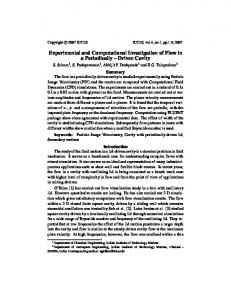
2.1 Network Model 2.1. 1 LSM Image An image based model of a precapillary arteriole was created using laser scanning microscope images (Figure 9) provided by the University of Rochester, Department of Ophthalmology, University of Rochester Medical Center, Rochester, NY. The pictures are of the choroidal vasculature of macaque monkeys affected by glaucomatous degeneration. These primates are used as test subjects due to the remarkable similarity between their vascular networks and that of a human. To develop the model, these images were viewed with the LSM image browser. Once a photo was selected for the foundation of the model, it was saved as a bitmap and opened using PAINT.net (www.getpaint.net). The program allowed an outline to be created of the choroidal circuit as a separate layer, which was then used as the bitmap file for the custom Matlab code.

2.1.2 Matlab The outline was then imported into Matlab® (Natick, Mass) as a bitmap where a custom program was used to capture the individual curves as a series of x-y points, one pixel per point where one pixel = 1.6 µm (Figure 9). The coordinates for each curve were saved as a text file. Each curve had to be captured individually and could not have repeating x-values due to the limitations of the Matlab code. This means that many curves were captured as a collection of smaller curves and stitched back together manually using Excel.

16

Figure 9: Left: An LSM image of the choroidal vasculature of a glaucomatous macaque. Right: An outline created to capture the curves using Matlab.

2.1.3 Excel Each text file containing the curve points was opened in Excel and plotted to affirm there were no outlying points. Many curves had to be manually smoothed due to the large percent error created by using a bitmap grid as a point system for generating the curves. Many curves appeared to oscillate ± 1.6 microns which created an accordion like section within the vasculature. The sharp edges would never be found in vivo and thus needed to be smoothed out for a more realistic network to be created. The curves were smoothed by creating an x-y plot in Excel with the pixel locations and removal the outlying points. If the plot still did not appear smooth, points were added back into the data set manually to create a smooth curve. Figure 10 shows the oscillating curve before and after smoothing. Unsmoothed

Smoothed

Section

Section

Figure 10: Left: Shows the pre-smoothed oscillation on a section curve. Right: Shows the same curve after the smoothing process. 17

Many individual curves also had to be manually stitched back together. Each curve was combined into a single x-y profile and any overlapping sections were deleted. Each curve also had to be placed in proper sequence or large discontinuities were seen. Once combined, an additional manual smoothing operation was repeated to ensure consistency with in vivo geometries. Finally, a z-dimension of zero was added to each point to fit the form of the x-yz coordinate system needed to import the curves into SolidWorks® (Concord, Mass). All coordinates were saved in a .txt file and imported into SolidWorks.

2.1.4 SolidWorks Once a curve was imported into SolidWorks, a splined centerline was drawn. The centerline was used as the path for a swept base while the imported curve was used as a guide curve. This allowed for the radius of the section of vasculature to vary with respect to the estimated centerline. Only one side of each curve was used as a guide curve, creating a radially symmetric model normal to the centerline as seen in Figure 11. The curves were imported from largest to smallest, with respect to the radius of the section of vasculature, to make the creation of a continuous model much simpler. Importing in this order made it easy to see that the end of the generated curve was completely encased in the previously generated larger curve. If the curve was not imported in sequence and not encased, the correct sweep and corresponding guide curve had to be relocated and edited. An additional point or series of points had to be placed onto the guide curve .txt file extending the end into the larger section of vasculature. The curve then needed to be re-imported and the sweep repeated until the proper position was achieved. Once all the curves were created the finished part file was saved as an IGES file (.igs) and imported into Gambit.

18

Figure 11: 3D model of the vasculature in Solidworks.

2.1.5 Gambit Once in Gambit, the model was split down the center x-y plane and the remaining faces were deleted. This new face, the x-y plane, was used for the 2D model. The amount of memory needed for the 3D network model exceeded the capability of the lab computer and therefore, the 2D model was used. A boundary layer was set at the internal edges to increase the accuracy along the wall. The mesh had to be created from the outside inward such that the sections with no branches coming off were meshed first. The sections that these branches flowed into or received flow from were then meshed and so on (Figure 12). The mesh was created with a boundary layer along the entire length of the model walls. The first row had an interval size of 0.05 μm with a growth factor of 1.1. The boundary layer thickness consisted of 8 rows with internal continuity. The lumen faces were meshes using an interval size of 0.5μm and a quadrilateral submap meshing scheme. The interval size method creates the number of nodes by dividing the length of the wall by the specified spacing interval. If the number of nodes is not an integer Gambit will round up to the nearest whole number. The final mesh consisted of 387492 quadrilateral cells. The mesh was imported into FLUENT® (ANSYS, Canonsburg, Pa) for computational analysis.

19

Figure 12: A 2D meshed model of the flow network in GAMBIT

2.1.6 FLUENT CFD analysis was performed using FLUENT. The fluid specified was a user created fluid exhibiting blood properties. The model was scaled from meters to microns and a scaling factor of 1.6 μm/pixel was specified to match the scaling of the LSM image. The pressure inlet was set to have an initial velocity of 6 cm/s [28]. Defining the pressure inlet finished the creation of the large 2D image-based network model of the precapillary arteriole network located around the ONH (Figure 13). A 3D model could easily be created using the same steps if a sufficient computational resource were available to run the CFD calculations.

Figure 13: A velocity contour plot of the 2D flow network in FLUENT. 20

2.2 Transport and Reactions 2.2.1 General Mass Transport in FLUENT To simulate mass transport, the UDS and UDF tools built into FLUENT were used. The UDS function used the general mass transport equation as defined by FLUENT: (1)

The general mass transport equation as defined by FLUENT where Φ represents the dependent variable, Γ represents the diffusion coefficient, and F represents the convection term ρU. S represents the user defined source term created in C++. The UDS function within FLUENT allows the user to create up to 50 species for transport and allows the user to simulate convective as well as diffusive properties of each chemical species. Transport properties can be adjusted for each cell zone and model layer. Only two species were used in this study, specifically oxygen and nitric oxide. The UDS is a way to create a species concentration and have the benefit of specifying different diffusion coefficients for different solid and fluid materials used in the simulation. The convective term is also defined by the user as well as the boundary conditions on the wall, inflow and outflows or pressure inlets and outlets. One powerful FLUENT capability is that a UDF source term can be created for each species reaction term and layer. This allows the user to code in C++, using predefined macros in ANSYS, to greatly simplify coding the species reaction terms for each individual layer. There are 18 general purpose UDF macros and 13 discrete phase modeling macros predefined by FLUENT allowing the user to easily modify properties of the UDS. The macros used in this study were the source term and profile macros. The source term macro 21

was used to create the Michaelis-Menten reaction terms while the profile was used to create the pulsatile flow velocity profile.

2.2.2 Chemical Reaction Source Terms For the source terms, a UDF was created for each species reaction and individual model layer. The UDF were based on Michaelis-Menten reaction kinetics model that was implemented for simplicity and ease of manipulation. The basis of this model is that the reaction rate is related to the concentration S of the species. The Michaelis-Menten kinetics general equation can be seen in Equation 2. (2)

V

Vmax S Km  S

Where V is defined as the reaction rate, Vmax is the maximum rate of reaction, and Km is the substrate concentration where the reaction rate V is at half of Vmax. The values used for Vmax and Km were previously specified by Lamkin-Kennard et al [12] [14] [15] and can be seen in Table 1.

2.2.3 Simple Models 2.2.3.1 Tube Model A five layer (lumen, plasma region, endothelium, vascular wall, and tissue) axially symmetric straight tube model was first created for simplicity and preliminary studies. Each layer had a UDS term for each of the chemical species as defined by Lamkin-Kennard [12]. The results from that paper were replicated in order to verify that the UDS codes were working correctly.

22

Figure 14: Simple 5-layer tube model from Lamkin-Kennard [12]. 2.2.3.1 Five Layer Model 2.2.3.1.1 Lumen (Fluid) The first layer, the vessel lumen, was defined with a radial distance of 50 µm. Flow in this layer was modeled as slug flow, with zero shear stress on the wall. Slug flow was simulated to mimic the Fåhraeus effect in which the red blood cells (RBCs) bunched up around the centerline due to the Fåhraeus effect. NO and O2 were subjected to both convective and diffusive transport. The lumen layer included the scavenging of NO due to reactions with hemoglobin in the RBC’s. The hemoglobin scavenging rate λb, was taken from Chen and Beurk (382.5 s-1) [22]. The mass transport equation with the hemoglobin scavenging source term (Equation 4) can be seen in Equation 3. (3) DNOb d dC NO (r )  b C NO  0 r dr dr (4)

b  k b C Hb In Equation 4, the NO hemoglobin scavenging source term, Λb is the reaction source term where kb is the hemoglobin scavenging rate and DNOb is the diffusion rate of NO in blood. 2.2.3.1.2 Plasma (Fluid) The next layer built into the model was a thin plasma layer. The plasma layer was an RBC free layer and was present to simulate the Fåhraeus effect. This layer was assumed to have a constant two µm thickness which acted as a buffer zone for the hemoglobin scavenging of NO. The plasma layer allowed NO to diffuse into the fluid flow without being immediately 23

consumed by the RBC’s. To simulate the fully developed velocity flow profile, a no slip condition was imposed at the outer edge and a constant shear stress of zero was set at the inner edge. NO and O2 were subjected to both convective and diffusive transport but chemical reaction UDF’s were not needed in this layer. 2.2.3.1.3 Endothelium (Solid) The third concentric layer modeled, the endothelium, was the first solid layer in the model. The endothelium was assumed to be two µm thick and included both O2 and NO reactions. The creation of NO was coupled to the bioavailability of O2. The Michaelis-Menten NO production rate RNO was defined in Lamkin-Kennard [12] and can be seen in Equation 5. The mass transport equation with an O2 consumption source term in the endothelium is seen in Equation 6.

RNOe  (

(5) R NOmax CO2

CO2  K m,eNOS

)

(6) DO 2 e d dCO2 (r )  RNOe  0 r dr dr (7) DNO e d dC NO (r )  RNOe  0 r dr dr Equation 7 is the NO mass transport equation in the endothelium with a NO generation source term where RNOe is the generation rate of NO in the endothelium while DO2e and DNOe are the diffusion coefficients of O2 and NO in the endothelium. NO generation was assumed to be uniform within the endothelium and dependent on the O2 concentration as well as the eNOS Michaelis-Menten reaction rate, km. Again these values were taken from Lamkin-Kennard [12]. The general mass transport for O2 and NO in the endothelium can be seen in Equations 6 and 7.

24

2.2.3.1.4 Vascular Wall & Tissue Layer (Solid) The fourth and fifth layers, the vascular wall and tissue, had thicknesses of 9 and 100 µm respectively. The concentration equations were identical for the different layers and the NO concentration was calculated by solving Equation 8. Equation 8 shows the NO mass conservation equation with an NO generation source term and a smooth muscle cell NO scavenging source term. This was calculated within the vascular wall and tissue. (8) Dt d dCNO (r )  t CNO  RNOe  0 r dr dr (9)

RNOe  (

R NOmax CO2 CO2  K m,eNOS

) And t  k sGC C sGCt

The left side of Equation 9 shows the NO generation term for the vascular wall and tissue layer. This term is typically zero unless iNOS or nNOS is present. The right side of equation 9 shows the scavenging rate of sGC for the vascular wall and tissue layer. In equations 8 and 9, the λt term, right side of Equation 9, represented the NO scavenging by soluble guanylate cyclase (sGC) found in the vascular smooth muscle cells. The rate of sGC scavenging (10 s1

) was also taken from Chen and Beurk [22]. The production rate of NO was zero in this

layer unless other NOS, iNOS or nNOS forms were present. A modified O2 mass conservation equation to incorporate Henry’s law of partial pressures and a maximum O2 consumption rate to use the inhibitory effect of O2 consumption with NO concentration is seen in Equation 10. Equation 11 shows the Michaelis-Menten reaction term for the reverse inhibition of O2 consumption by NO.

(10) DO 2 S O2 d dPO 2 PO 2 (r )  Qmax 0 r dr dr PO 2  AppK m

(11) 25

AppK m  Km(1 

C NO ) 27 nM

Equation 10 and 11 incorporate Henry’s Law of partial pressure and take into account the concordant oxygen solubility, SO2. AppKm represents the inhibitory effect of NO on O2 consumption and increases linearly with NO. Qmax represents the maximum rate of O2 consumption and was the only difference in the mathematical representation of the two layers.

Figure 15: Section of the axial symmetric simple tube model. Blue depicts the solid layers while red depicts fluid layers. All dimensions are in microns.

Figure 15 shows a section of the 2D axially symmetric tube model created for FLUENT with the different layers labeled. Flow and reactions were simulated with an axis-symmetric condition at the bottom of the lumen as the axis. All dimensions were in microns, mimicking the model used by Lamkin-Kennard [12]. The three blue sections represent solid areas with no blood flow. The two red sections represent fluid areas where convective transport occurs for both chemical species. Table 1 below shows the constants used in the model.

26

Table 1: Parameters used in the model. Definition Value Units Vessel Geometry 762.5

μm

50

μm

2

μm

Endothelium

2

μm

Vascular Wall

9

μm

Tissue Thickness

100

μm

Hematocrit

45

%

Solubility Coefficient

1.3

μM Torr-1

Vessel Length Lumen Diameter Plasma Layer Thickness

Diffusion Coefficients O2

2800

μm2 s-1

NO

3300

μm2 s-1

Maximum O2 Consumption (Qmax) Vascular Wall

5

uM s-1

Tissue

50

uM s-1

382.5

s-1

10

s-1

54

μM s-1

Hemoglobin Scavenging of NO (λb) Tissue Scavenging of NO (λt) Maximum eNOS Production (RNOmax)

Km for O2Dependent NO Production eNOS

4.7

Torr

iNOS

3.8

Torr

nNOS

15

Torr 27

2.2.3.2 T-Geometry

Figure 16: The dimensions and layers of the T-geometry model created for FLUENT. All dimensions are in microns and red represents the fluid sections while blue indicates the solid sections.

The second model tested was the T-Geometry, Figure 16, which was created to maintain the five layers of the simple tube model seen in Figure 15. This was created to simulate a 90 degree bifurcation in the vascular network. The layered structure allowed for the ease of implementation of the UDF reaction terms that had already been created. The UDF source terms were imported into this new geometry and functioned correctly without any manipulation of the equations. This model was created in 2D with a symmetric boundary condition along the bottom of the lumen.

28

2.2.3.3 Y-Geometry

Figure 17: The dimensions and layers of the Y-geometry model created for FLUENT. All dimensions are in microns and red represents the fluid sections while blue indicates the solid sections.

The third model tested was the Y-Geometry, Figure 17, which again maintained the five layers of the previous geometries tested. Maintaining the layers allowed for simple implementation of the UDF reaction terms that had previously been created and simulated in the Tube and T-geometries. The Y-model was created in 2D with a symmetric boundary condition along the bottom of the lumen. The Y-bifurcation consisted of a 45° angle. 2.2.3.4 Table of Equations The Tube model was simulated using an axis symmetric boundary condition and the equations were in cylindrical coordinates. The mass transport equation was converted to rectilinear converted to rectilinear coordinates for the T and Y-geometry models as well as the layered network model. The conversion was necessary because an axis symmetric boundary condition could not be imposed due to the bifurcations. Table 2 lists the mass transport equations solved by layer for both O2 and NO.

29

Table 2: Transport equations with the source terms solved in the X and Y direction for each layer.

30

2.2.4 Boundary Conditions

Figure 18: Boundary conditions specified in FLUENT. Flow will move from left to right via the pressure inlets 1 and 2. 2.2.4.1 Lumen Boundary Conditions The lumen had four different boundary conditions associated with it as shown in Figure 18. The bottom of the rectangle was designated as a symmetry boundary condition, therefore the radial symmetry of the tube allowed a simple 2D face to be used. A zero shear stress condition was thus imposed on the bottom wall,   0 , to allow the max velocity of the parabolic profile to be at the centerline. For the UDS boundary condition, the symmetry condition means that there is zero flux in the y-direction across the boundary which is modeled using Equations 12. (12)

 D0

dC 0  0 &  D1 dC1  0 . dy Lumen dy Lumen

The top, outer edge, of the lumen was modeled as a coupled-wall with a boundary condition that allowed UDS flux out to equal the UDS flux into the plasma layer such that

 Dn

dCn dCn  Dn (Table 2). The coupled wall condition allowed for the flow field dyLumen dy plasma

boundary conditions in the lumen to be different than the wall boundary condition for the

31

field flow in the plasma layer. There was a no slip condition, u=v=0, on the upper wall to create the parabolic velocity profile. The left side was designated as the pressure inlet, which allowed for a constant pressure to be imposed on the left side of the lumen which generated the velocity profile in the lumen. The pressure inlet was also used to input the UDS concentrations. The UDS boundary value was specified allowing the concentration to be constant at the pressure inlet. The right side of the lumen was designated as a pressure outlet with gauge pressure. The UDS concentrations were calculated at the pressure outlet. Table 3: Equations simulating the boundary conditions of the lumen.

2.2.4.2 Plasma Boundary Conditions For simplicity, the plasma layer was modeled as a solid but still maintained the 2 μm NO diffusion buffer from the Fåhraeus effect for RBC NO consumption. The upper and lower edges of the plasma layer were modeled as walls and used the same conservation principle as applied between the lumen and endothelium wall: flux in is equal to flux out. For the lower wall, the flux into the plasma layer was equal to the flux out of the lumen. On the upper wall, the flux out of the plasma layer was equal to the flux into the endothelium (Table 3). These fluxes are represented mathematically in Equations 13. (13)  Dn

dCn dCn  Dn dyPlasma dyEndothelium

 Dn

dCn dCn  Dn dyLumen dy plasma

Table 4: Equations simulating the boundary conditions of the plasma layer.

32

The left and right edges were modeled with a symmetry boundary condition which maintained 0 UDS flux across the wall and created a 0 UDS gradient in the x-direction.

2.2.4.3 Endothelium Boundary Conditions The upper and lower bounds of the endothelium were modeled using wall conditions with continuity at the boundary, such that flux in = flux out. The lower wall was modeled by setting the flux out of the plasma equal to the flux into the endothelium and the upper wall was modeled as the flux into the vascular wall equal the flux out of the endothelium (Table 4). These fluxes are represented mathematically in Equations 14. (14)

 Dn

dCn dyEndothelium

 Dn

dCn dyVascularWall

 Dn

dCn dCn  Dn dyPlasma dyEndothelium

The left and right side were modeled as symmetry boundary conditions so that there was no UDS gradient in the x-direction across the designated boundaries. This boundary condition is represented mathematically in Equation 15.

 Dn (

(15) dCn

dxEndothelium

)0

Table 5: Equations simulating the boundary conditions of the endothelium.

33

2.2.4.4 Vascular Wall Boundary Conditions The upper and lower bounds of the vascular wall layer were modeled using continuity of flux. The lower wall was modeled by setting the flux out of the endothelium equal to the flux into the vascular wall. The upper wall was simulated by setting the flux out of the vascular wall equal to the flux in the tissue layer (Table 5). These fluxes are represented mathematically in Equations 16. (16)  Dn

dCn dyVascularWall

 Dn

dCn dyTissue

 Dn

dCn dyEndothelium

 Dn

dCn dyVascularWall

The left and right side were modeled using symmetry boundary conditions which did not allow for UDS flux in the x-direction across the designated boundaries. The symmetric boundary condition is represented with equation 17.

 Dn (

(17) dCn dxVascularWall

)0

Table 6: Equations simulating the boundary conditions of the vascular wall.

34

2.2.4.5 Tissue Boundary Conditions The tissue layer was modeled using a wall condition with zero flux on the upper bound. This restricted the diffusive area of the entire model to a maximum of 163 microns in the y direction from the centerline. The lower bound had a matching flux condition, where the flux out of the vascular wall was equal to the flux into the tissue layer (Table 6). The fluxes are represented in Equations 18. (18)  Dn

dCn dyVascularWall

0

 Dn

dCn dyVascularWall

 Dn

dCn dyTissue

The left and right sides had a symmetry condition which only allowed the UDS concentration to change in the y- direction. Table 7: Equations simulating the boundary conditions of the tissue.

2.3: Layered Network Model 2.3.1 SolidWorks The SolidWorks model described in section 2.1 was used as the platform to generate a layered network model. However, the complexity of the previous model would violate some of the assumptions made such as the constant thickness of the vascular wall, (nine µm). One example is a section of lumen with a maximum distance of 5 microns between another section of lumen. This would not allow for the plasma layer, endothelium, and vascular wall layers to be created. Therefore, only the main lumen section and 12 branches were used for the layered network model (Figure 19). This proof of concept was designed to show that it is

35

possible to create a relatively simple layered model which could provide the foundation for a more complex layered model in the future.

Figure 19: Simplified network model.

To create the layers in the network, a sketch was created in the front plane which split the model down the x,y plane. The outer line of the section of vasculature to be layered was then offset. In the simple models the thickness of the plasma and endothelium was 2 μm and the vascular wall was 9 μm. To maintain this thickness the offset values had to be divided by 1.6 to compensate for 1 pixel being equivalent to 1.6 μm. Therefore, the offset values used for the creation of the layered network model were 1.25 and 5.625 μm. Once the offset was created, a swept base was used as described previously in the creation of the network model in Section 2.1. The same centerline used to section the vasculature was used and the new offset curve was used as the guideline. The merge result option for the swept base was unchecked so that the layers did not appear as one volume when imported into Gambit. If this was not unchecked, only the outer most edge would be seen in Gambit and the multiple layers inside would have seemingly disappeared. The tissue layer was not created in SolidWorks using an offset. The tissue layer does not have a relatively constant thickness in-vivo, rather it fills the gaps between the vasculature. The creation of the tissue layer was created later once the model was imported into Gambit. 36

2.3.2 Gambit The completed layered (plasma, endothelium, vascular wall) model was imported into Gambit as an .iges file. The model was then split down the center and all remaining volumes and faces were deleted to create the 2D model. The 2D faces were then deleted leaving all lower geometry. The lines were split at each intersection allowing for the creation of continuous faces of the lumen, plasma, endothelium, and vascular wall as seen in Figure 20. The faces were then recreated and the faces were categorized into the correct cell zones as seen in Figure 21.

Figure 20: 2D layered network model in Gambit.

Figure 21: The layered network model showing the fluid layers in red, the endothelium and vascular wall in blue, and the tissue layer in black. Note that both blue and black 37

correspond to solid layers. The right side of the model is the pressure inlet which creates the flow from right to left.

The tissue layer was not created using an offset of 100 microns from the vascular wall. This was because the constant thickness is simply unrealistic when compared with in-vivo geometries. The tissue layer fills the gaps between branches despite thickness and shape. FLUENT does not allow velocity or pressure outlets to be set next to solid cell zones. Therefore, the tissue areas were created by connecting the points of the vascular layer that lie on the same plane as the pressure outlets and the pressure inlet. Some locations had to be offset as to not intersect protrusions of the vascular wall. The tissue layer can be seen by the black sections in Figure 21. The lumen, plasma layer, endothelium, and vascular wall were meshed with 40378, 12027, 12102, and 40137 quadrilateral cells respectively. The tissue layer was meshed with 120149 mixed cells, quadrilateral and triangular, due to the irregular shape of the tissue faces. The interval spacing ranges from 0.5 to 1.35 μm creating a range of resolutions of 0.25 to 1.8225 μm2. The completed grid was exported into FLUENT for CFD analysis.

2.3.3 FLUENT Once the mesh was imported into FLUENT, the mesh was scaled at 1.6e-6 to change from meters to microns and so that one pixel equaled 1.6 microns. The grid was checked for skew violations and the boundary conditions used in the simple models were then imported into the layered network model for consistency.

38

Figure 22: Velocity contour plot of the 2D lumen in the layered network model.

A pressure was set into the pressure inlet boundary condition and the velocity contour plot was generated (Figure 22).

2.3.4 C++ Source Terms The source terms were created with a UDF using a predefined macro called DEFINE_SOURCE (name, c, t, dS, eqn), seen in Figure 23. FLUENT has defined this macro to specify custom source terms for the different transport solvers within the program, including the UDS. The name is specified by the user and will be visible within the cell zone UDF arguments after the code is compiled or interpreted. The variable t is a pointer to the cell thread and c is the cell to which the source term will be applied. dS is an array specifying the derivative of the source term with respect to the dependent variable of the transport equation. This derivative may be used to linearize the source term which may enhance the stability of the solver. Eqn denotes the equation to be returned as the source term value. The DEFINE_SOURCE macro did not need a loop as the macro automatically calculated the source term for each cell within the specified cell zone. The UDF C++ code also uses the predefined variable for the UDS concentrations. The variable C_UDSI(c,t,i) was used in the equations to denote the UDS species. t and c defined

39

the thread and cell as before where i denoted the UDS number where 0 represented oxygen and 1 was nitric oxide. The source term RNOe, Equation 6, was coded using C++ and can be seen in Figure 23. To avoid any confusion with the scalar indices, 0 and 1, the numbers were reassigned as oxygen and NO which can be seen on lines six and seven of Figure 23. The constants RNOmax, KmeNOS, and AlphaT were defined in lines 15, 16, and 17 respectively. The equation was replicated in line 26 for NO generation and the value was returned in line 28 to FLUENT as the generated value. The O2 consumption term was calculated and converted to Torr in line 37 and returned to the mass transport equation in line 39.

Figure 23: The C++ code for the RNOe Source terms for NO generation and O2 consumption in the endothelium. 40

The RBC scavenging source term, Equation 4, was coded in the same process and can be seen in Figure 24. Line 77 defined the Λb, RBC scavenging rate, as a constant 382.5 –s. In line 84 the full equation was defined and was returned as the source term in line 86.

Figure 24: C++ coding for the RBC scavenging, Equation 4, source term in the lumen.

The vascular wall NO consumption source term, Equation 9, was replicated in C++ in line 103 of Figure 25 using a NO scavenging rate constant, λvasc, of 10-s, defined in line 96. The O2 source term, right side of Equation 10, was defined in line 120. The AppKm constant, Equation 11, was put directly into the equation, but was noted in line 118. The constants Km, Qmax, and Cref for the vascular wall were defined in lines 109,110, and 111 respectively.

41

Figure 25: C++ code for the NO generation and O2 consumption in the vascular wall.

The tissue layer NO consumption source term, Equation 9, was replicated in C++ in line 103 of Figure 26. An NO scavenging rate constant, λtissue of 10-s , defined in line 131. The O2 source terms, Equation 10 and 11, were defined in line 155. The constants Km, Qmax, and Cref for the vascular wall were defined in lines 144,145, and 146 respectively.

42

Figure 26: C++ code for the NO generation and O2 consumption in the tissue.

2.3.5 Initial Conditions 2.3.5.1 Steady - State The steady-state solution was completed by allowing FLUENT to repeat the iterations until the dependent variables converged to a solution independent of a time step. The study used the pressure inlet, which allowed for the input of a pressure, in Pascals, to exhibit a constant driving force for the flow field. The pressure was set to create velocities of 6, 3, 1, and 0.15 cm/s in the lumen to simulate multiple velocity profiles. The UDS was set to “Specified Value” for UDS-0, O2, and a UDS boundary value was input at 80 Torr. These simulations used the partial pressure of the oxygen, PO2, as a constant at the pressure inlet. Convergence was monitored for the velocities in the x and y directions. The UDS convergence and the continuity were also monitored to ~ 1e-16. The plasma layer pressure inlet had the same defined properties as the lumen, however there was no UDS concentration input. The pressures that were input created velocity profiles

43

with maximum velocities of six, three, and one cm/s. This allowed for a wide range of flow profiles to be simulated. 2.3.5.2 Ischemia Simulating ischemia was also required to test the possibility of the flow abnormality causing elevated NO. The UDS concentrations for the lumen, plasma, endothelium, vascular wall, and tissue layer had to be written separately from the steady state solution. The separate UDS data was required to simulate the sudden cessation of flow within the lumen while still containing species concentrations. The cessation of flow can be represented mathematically by the general mass transport equation with the convective term going to zero as seen in Equation 19. (19)

  xi , j

( ui , j C0  D0

C0 C0  )  S 0L  0  ( D0 )  S 0L  0 xi , j  xi , j xi , j

The ischemic simulation was completed using the interpolate function in the File dropdown menu. The interpolate data options were selected as write data and the variable fields were selected as UDS-0 and UDS-1, Oxygen and Nitric Oxide. The cell zones were listed in alphabetical order and therefore endothelium was selected as the first cell zone. The file was written and saved and this process was repeated for every remaining cell zone (lumen, plasma layer, tissue layer, and vascular wall). The pressure inlets and outlets were set to symmetry to allow for the fluid to be stagnant and emulate an ischemic region where flow had suddenly been blocked. The symmetry boundary condition also eliminated any initial conditions which could add UDS concentrations. When the pressure inlet and outlet conditions were changed to symmetry, FLUENT indicated that the x and y velocity profiles have converged and stopped the simulation because there is no velocity change. To avoid the calculation complete window in FLUENT, the monitors for x and y velocities must be turned off or the 0 change in velocity would satisfy the convergence condition. To decrease the calculation time, continuity was also turned off so the UDS concentrations were the only remaining convergence terms.

44

The solution was then initialized and the cell zone concentrations were restored onto the nodes using the written interpolated files. Run was hit six times because the first five iterations do not contain the UDS function and therefore, solution converged window would repeatedly come up on the screen. 2.3.5.3 Reperfusion To simulate reperfusion the UDS concentrations were written from the ischemic simulation. The interpolation steps were repeated to write the UDS concentrations at each cell. The lumen and plasma pressure inlets were restored and then adjusted to resume the original velocity profiles and UDS concentration. Readjusting the pressure inlet involved reapplying the pressure that was used previous to the ischemic simulation and setting UDS-0 to a constant 80 torr. The reapplication of the velocity term can be shown mathematically by the mass transport equations convective term going from zero to non-zero as seen in equation 20.

  xi , j

( D0

C0 )  S 0L xi , j

(20) C0  0 ( u i , j C0  D0 )  S 0L  0  xi , j xi , j

The pressures at the inlets and the UDS concentration at the lumens pressure inlet were replaced to simulate blood flow returning to the vascular network carrying oxygen from the lungs. The simulation was then initialized and the UDS concentrations interpolated back onto the nodes. 2.3.5.4 Pulsatile Flow To create the pulsatile flow profile a sinusoidal curve with a constant offset was used as the foundation of the velocity profile. The mathematical representation of the profile exhibits the form of Equation 21 that (21)

V  vx  A * sin(w * t ) Where V is the total velocity and vx is the offset from zero or the center point of the sinusoidal curve. The νx offset was calculated by the mean of the peak systolic and the end diastolic velocities. A is the amplitude of the sinusoidal curve or the peak deviation from the 45

center point of the function and was calculated as one half of the difference of the peak systolic and end diastolic velocities. The ω is the angular frequency and specifies the number of oscillations per second of the function in radians. T represents the time at which the function is being evaluated. The values for the peak and end velocities come from Deokule et al [27] with a peak systolic velocity of 0.14 cm/s and an end diastolic velocity of 0.022 cm/s. The pulse rate was taken from K. Polak et al [28] with 64.9 beats per minute, bpm, which reduces to ~ 1.082 beats per second. The bpm rate means that an entire sinusoidal cycle needs to take place in ~ 1.082 seconds The mean (νx) was calculated using the velocities yielding a value of 0.00081 m/s. The amplitude, A, was calculated to be 0 .00059. The angular frequency was calculated using equation 22 and 23. Equation 22 calculated the angular frequency in radians/second while Equation 23 calculates the frequency using the period, or time for one cycle. (22)

  2f (23)

f 

1 T

The period was calculated to be 1.0817 seconds and the angular frequency was calculated to be 5.8088 rad –s. An estimate of the time step was made to be 0.054083 so that 20 time steps would complete a full cycle. 60 time steps, or three periods, were simulated and the velocity profile can be seen in Figure 27.

46

Figure 27: Pulsatile profile vs time for three cycles from the calculated values.

The velocity profile was created with a UDF using a predefined macro called DEFINE_PROFILE. This macro was used to define a custom velocity boundary profile that varied with time. The arguments for the macro are name, t, and i or DEFINE_PROFILE (name, t, i). The name is again defined by the user and was defined as Pulsatile as can be seen in Figure 28 line 11. t was again a pointer thread passed through FLUENT and i was the index identifying the variable that is to be defined. The position was used in this code and can be seen in line 11. The utility Current_Time was used to look up the flow time and was assigned to variable t. An f loop, or face loop, was used to calculate the velocity at all faces on the boundary.

47

Figure 28: C++ code for the pulsatile velocity profile.

The code was hooked to the velocity inlet boundary condition and the calculation was set to transient. A surface monitor was created on the velocity inlet so that a plot could be made of the area-weighted average of the velocity vs. time. The time step was set to 0.054083 and a maximum of 1000 iterations per time step was used. The velocity vs. time plot can be seen in Figure 29. Figure 29’s profile identically matches the velocity profile created in Figure 27.

Figure 29: Pulsatile velocity profile created in FLUENT. 48

Chapter 3: Simple Model CFD 3.1 Grid Independence Study 3.1.1 Tube Model 3.1.1.1 Velocity

A grid independence study was completed using velocity as the test variable and a no slip condition at the walls. The mesh was refined from an interval spacing of 9.25 to 0.45 μm. The spacing numbers also corresponded to 410 cells to and 187479 cells within the lumen. The velocity was taken along the height of the lumen at three-fourths the length of the vessel. The three-fourths length was used to allow the entrance length to be passed and the fully developed velocity profile to be used. The percent difference was calculated from the smallest interval spacing.

Figure 30: Percent difference between the velocity and the corresponding number of cells. The red circle encloses the point corresponding to the 2 μm interval spacing or the 9525 cell grid. This was selected as the interval spacing for the entirety of the tube model.

The red circle in Figure 30 encloses the percent difference between a 187479 cell mesh and a 9525 cell mesh of ~2.6 %, at the node three-fourths the length of the vessel. The percent difference value corresponds to a difference of 0.0002 m/s which has surpassed the “knee” of 49

the curve and is on the flatter section where the percent differences between intervals are consistently between 2.7-2.5 percent. Therefore, a mesh with ~ 2000 to ~180000 faces was within the grid independent solution. The final mesh for the simple tube model was mapped scheme with a 2 μm interval spacing for the lumen, vascular wall, and tissue layers. The lumen, vascular wall, and tissue contain 9525, 1905, and 19050 elements respectively with a resolution of 4 μm2. The plasma and endothelial layers were meshed using a 3 cell interval count on the vertical sides and maintaining the 2 micron spacing interval spacing along the horizontal sides. This created a mesh size of 1143 cells for both layers with a resolution of 1.333 μm2, 0.666 x 2.0 μm.

Figure 31: Contour plot of the velocity in the lumen.

In Figure 31, the lumen of the tube model was split down the center with a symmetry boundary condition and concordantly shows the fastest velocity at the center. The zero velocity seen along the upper wall was due to the no slip condition.

50

Figure 32: Velocity profile in the tube geometry. The left side of the x-axis corresponds to the centerline while the right side corresponds to the wall.

The plot in Figure 32 shows the velocity profile of the tube model. The left side of the x-axis corresponds to the centerline while the right side corresponds to the wall. This plot shows the correct parabolic shape of the velocity profile seen in Figure 2 of the Fåhraeus effect. 3.1.1.2- NO Concentration A grid independence study was also completed using the UDS-1, NO, as the test variable. The mesh was refined from an interval spacing of 4.25 to 1.25 μm which correspond to meshes with 7876 cells to 81130 cells. The peak value of the NO was taken and the percent difference from the 81130 cell mesh was calculated and plotted in Figure 33.

Figure 33: Percent difference in peak NO levels from the 81130 cell mesh. 51

The red circle encloses the spacing interval of 2 μm, 32766 cells was used as the final mesh for the tube model. The full details of the mesh were described in the previous section, 3.1.1.1. The percent difference was consistently around 1% for the 3 mesh sizes tested before the final 81130 cell mesh and was accepted to be within the grid independent solution.

3.1.2 T-Geometry- Velocity The same process was repeated for the T-geometry ranging the space interval of the mesh from 10.25 to 1.25 μm. The number of cells varied from 365 to 67000. The T-geometry induced a stagnation line in the intersection of the T as it should, suggesting that the CFD model was working as it should. Stagnation is a well known phenomenon in fluid mechanics created at a bifurcation of a flow field which generates a point of zero velocity.

Figure 34: Percent difference between the spacing intervals of the velocity. The red circle encloses the point corresponding to the 2 μm interval spacing or the 8990 cell grid. This was selected as the interval spacing for the entirety of the T- Geometry model.

The percent difference between the velocity solutions in the 67000 and 8990 cell meshes was ~0.17 % (Figure 34). The percent difference was sufficiently low and occurs after the “knee” of the graph. Therefore, the interval spacing of 2 μm and a mapped scheme was used as the final grid spacing for the T- model. The spacing is identical to the spacing that was used for the tube model. 52

The lumen, vascular wall, and tissue layers were meshed with a 2 μm mapped spacing interval corresponding to a resolution of 4 um2. The lumen, vascular wall, and tissue layers contain 8990, 2590, and 23150 cells respectively. The plasma layer and endothelium were again meshed with an interval count of 3 cells on the short side and an interval spacing of 2 μm along the length. This creates a resolution of 1.333 μm2, 0.666 x 2.0 μm.

Figure 35: A contour plot of the velocity in the lumen

To reduce computational time, the lumen was split down the center with a symmetry boundary condition on the horizontal section. This boundary condition everything splits evenly on the vertical section where both walls have the no slip condition. In Figure 35, the stagnation line can be seen as well as the areas of low speed flow surrounding it.

53

Figure 36: Left: Vector plot showing a close up of the intersection verifying the stagnation line and the surrounding area of low speed flow on the T-geometry. Right: A velocity contour plot highlighting the low speed flow area created by the 90° turn of the T-geometry.

In Figure 36, velocity vectors of the low speed flow area around the stagnation line can be seen. The stagnation line is easily seen by the contour plot of velocity. There is almost a stagnation layer created as the wall is approached from the centerline.

Figure 37 : Velocity profile at ¾’s the length of the horizontal section.

In Figure 37, the velocity profile of the T-geometry can be seen at three-fourths the length of the horizontal section of the lumen. The left side of the x-axis corresponds to the centerline 54

while the right side corresponds to the wall. Figure 37 verifies the correct parabolic shape of the velocity profile in the T-geometry.

3.1.3 Y-Geometry- Velocity The same process was again repeated for the Y-geometry with the space interval of the mesh ranging from 10.25 to 1.25 μm. The number of cells varied from 385 to 18072. The Ygeometry also induced a stagnation line in the intersection of the Y suggesting that the CFD model was working as it should.

Figure 38: Percent difference between the spacing intervals of the velocity. The red circle encloses the point corresponding to the 2.75 μm interval spacing or the 5480 cell grid. This was selected as the interval spacing for the entirety of the Y- Geometry model.

The percent difference between the velocity solutions in the interval spacing corresponding to 13361 and 5480 cells was ~1.4 % (Figure 38). The percent difference was sufficiently low and occured after the “knee” of the graph. Therefore, a mapped scheme and an interval spacing of 2.75 were used for the lumen, and vascular wall corresponding to meshes of 5480 and 18072 cells. The Tissue was broken up into 4 sections which can be seen in Figure 39. Section 1 and 3 were meshed with a spacing interval of 2.75μm which correspond to mesh sizes of 4608 and 3492 cells. Sections 2 and 4 were mapped with a quad element of tri 55

primitive type which created 855 and 5712 element meshes respectively. The total number of cells in the tissue layer is 14667 with an average resolution of 7.5625 μm2. The endothelium and plasma layer were once again meshed along the short side with an interval count of 3 and then maintained the 2.75 interval spacing of 2.75μm along the length. This created meshes of 972 and 990 respectively with a resolution of 1.333 μm2, 0.333x 2.75 μm.

Figure 39: Shows 4 sections of Tissue.

Figure 40: Velocity in the lumen ion the Y-geometry.

In Figure 40, the lumen has been split down the center with a symmetry boundary condition on the horizontal section. The symmetry boundary condition created a mirror image on the

56

opposing side which completed the geometry into a full Y shape. The symmetry boundary condition was used to reduce computational time.

Figure 41: A close up of the intersection verifying the stagnation line and the surrounding area of low speed flow on the Y-geometry.

Figure 41 depicts the area of low speed flow created by the split of the Y-geometry and also the contour plot of the velocity at the intersection. The 45° turn, Y-geometry, vs. the 90° turn of the T-geometry creates a much smaller area of low speed flow and a shorter stagnation line which can be seen when comparing Figures 36 and 41.

Figure 42: Velocity profile at three-fourths the length of the horizontal section.

The plot in Figure 42 shows the velocity profile at three-fourths the length of the horizontal section. The left side of the x-axis corresponds to the centerline while the right side corresponds to the wall. This plot verifies the correct parabolic shape of the velocity profile in the Y-geometry. 57

Chapter 4: Layered Network Model CFD 4.1 Grid Independence Study A grid independence study was also completed for the network model using velocity as the test variable. A no slip condition was used at the walls rather than the slip condition used to simulate slug flow during the final simulations. The slip condition was used to verify the accuracy of the grid because slug flow does not require such a refined mesh. However, species transport was conducted using the same mesh and therefore an adequately refined mesh was needed. For this study, the layered network model was reduced to a single layer representing just the lumen. The lumen was then split into separate pieces for flow simulation testing seen in Figure 43. The lumen was broken into 13 individual sections and new pressure inlets were set so that the flow would move in the same direction as it would in the completed model. Each section of the flow field was simulated individually for the grid independent study.

Figure 43: Lumen broken up into separate pieces for the grid independence study. Each color signifies a separate section.

Each velocity contour plot was closely examined for each meshing scheme to look for any non-intuitive flow patterns in each of the sections. Any abnormalities resulted in a complete remesh of the section, often involving breaking original face into many smaller sections.

58

Because of the wide range of diameters throughout the various sections, it was not feasible to place all the resulting curves on the same plot using the same number of cells as the x-axis. Therefore, a new method of plotting had to be created to fit each curve onto the same plot. The collective interval spacing ranged from 3.25 to 0.2 μm and each interval was given a corresponding number as seen in Table 1. The varying areas of the different sections cause the number of faces to range from 42 to 9500 per branch. When the faces were plotted on the same graph the x-axis was far too large to place on a single page. As a result, the spacing intervals were numbered one to seven from the largest spacing interval, 3.25, to smallest of .2, as seen in Table 8. Table 8: Spacing interval (S.I.) with the corresponding plot number. Space Interval

S.I. plot number

3.25

2.25

1.25

0.75

0.5

0.25

0.2

1

2

3

4

5

6

7

The plot was created showing the percent difference of the velocity at one-fourth the length of the pressure outlet of each section of vasculature. The plots (Figure 44) were not completed as far out as the previous curves due to the computational time for each simulation, but through experience and intuition it was deduced that the curves are down to the knee of the curve or later.

59

Figure 44: Percent difference for each section of vasculature corresponding by color to Figure 40.

In Figure 44 all the curves reached an acceptable percent difference at the conclusion of the grid independence study. When the sections were meshed, the smallest spacing intervals were meshed first. In a small number of instances this caused the next section to be meshed at a point further down the curve (beyond those seen in Figure 44). However, the number of faces did not increase so much as to disrupt the validity of the grid independence study. To mesh the other layers (plasma, endothelium, and vascular wall) in a mapped fashion, the same interval spacing was often used as the adjacent section of lumen. The spacing intervals for these layers were all smaller than the grids generated for the simple models and intuitively it can be said that this will provide an acceptable solution. To create a meshed scheme, the majority of the faces had to be broken into several smaller faces and added to the cell zone designations. Many faces also had highly skewed cells which resulted in poor solution data. Each of these skewed cells were corrected, often involving creating additional faces and occasionally using a non-mapped meshing scheme. The lumen, plasma layer, 60

endothelium, and vascular wall were meshed with 40378, 12027, 12102, and 40137 quadrilateral cells respectively. The tissue layer was meshed with 120149 mixed cells, quadrilateral and triangular, due to the irregular shape of the tissue faces. The interval spacing ranges from 0.5 to 1.35 μm creating a range of resolutions of 0.25 to 1.8225 μm2. The tissue sections were meshed with a quad or tri paved scheme as a result of the abnormally shaped faces. The completed meshed layered network model can be seen in Figure 45.

Figure 45: Depicts the completed mesh for the layered network model.

As shown in Figure 46, the resulting velocity profile looks reasonable having the fastest flows in the main lumen near the pressure inlet. The velocity slowly decreases as more area is available via the branches and in addition the pressure drops towards the pressure outlets (Figure 46).

61

Figure 46: Left: Velocities, m/s, in the layered network model with the grid independence study meshing scheme. Right: The right contour plot shows the drop in pressure, Pa, stemming from the pressure inlet on the right to the pressure outlets at the ends of the branches.

The velocities within the branches are significantly slower than the main branch of the lumen as seen in Figure 47. To verify that the mesh was working correctly the velocity was scaled down show the maximum velocity within the branches. This can be seen in Figure 47 which shows the velocity profile is still correct within the branches. The fastest velocity is in the center of the branch while the walls remain at zero velocity due to the no slip condition imposed at the wall for the grid independence study.

Figure 47: Contour plots of the velocity, m/s that was scaled to show the profiles within the branches.

62

Chapter 5: Simple Model Results Chapter 5 goes into the detailed results of the simple geometry flow models with the coupled O2 and NO transport and reactions. The uncoupled O2 transport results are presented for each geometry, presenting the results for each flow abnormality. Then, the results are presented for the coupled transport of O2 and NO for the simple geometries under each flow abnormality.

5.1 Oxygen Transport 5.1.1 Tube Model 5.1.1.1 Comparisons The code from Lamkin-Kennard [29, 12] was run in FlexPDE for comparison of the O2 partial pressures for an arteriole with a radius of ten microns and a velocity of 0.15 cm/s. The PO2 distribution was taken at nine microns into the vessel (Figure 48). FLUENT was not able to converge a solution for the UDS using the slug flow and the liquid plasma layer. Consequently, the plasma layer was set to solid and a no slip condition was imposed on the wall to maintain a parabolic velocity profile.

63

Figure 48: Distribution of the PO2 from the code used to create Lamkin-Kennard [29].

In Figure 48, the y-axis increments at a rate of 0.001 Torr. The value of PO2 is constant until approximately one micron before the plasma layer and results in a total change of ~ 0.00025 Torr. This corresponded to ~0.002 % suggests that a constant value of O2 should be seen in the lumen. The diffusion coefficient does not change within the different layers of the model and therefore, an almost constant value of O2 should also be seen throughout the geometry. This assumption was only valid before any metabolic O2 consumption source terms were used. To compare with the graph in Figure 48, the model was replicated in FLUENT. The PO2 distribution was plotted at nine microns into the geometry and is seen below in Figure 49.

64

Figure 49: Distribution of the PO2 across the lumen from FLUENT replicating the plot in Figure 48.

The PO2 values generated by FLUENT show a constant PO2 across the lumen with a total percent difference from Lamkin-Kennard [29] of 0.00025%. This is an acceptable value and verifies that the oxygen transport model is working correctly in FLUENT. The major difference in these models is that the FLUENT simulation also included a convective term. 5.1.1.2 Steady-State Tube Model 5.1.1.2.1 Comparing Changes in Velocity The velocity was varied from 6 cm/s to 0.15 cm/s (6, 3, 1, 0.15) and the PO2 was plotted. The rapid convection and diffusion rate of the O2 and fixed value of 80 Torr at the inlet created a constant concentration throughout the tube which can be seen in the contour plot in Figure 50.

Figure 50: Contour plot of the PO2 throughout the simple tube model with a radius of 50 microns. 65

The percent difference of PO2 between the 6 cm/s simulation and the 0.15 cm/s simulations was zero. If the velocity was going to be a factor in the PO2 concentration then a comparison between these two velocities should show the largest difference in concentration.

The zero

percent difference finding verified the assumption from section 5.1.1.1.1 that a constant value of O2 would be available for metabolic processes within the tube.

Figure 51: Plot of the PO2 across the tissue at three quarters the total height of the 50 micron radius model.

Figure 51 shows the continuous concentration of O2 at three-fourths the height of the tube and within the tissue layer. This graph is identical for the different velocity simulations and therefore, only one was plotted. 5.1.1.2.2 Steady-state, Changes in Radius The change in radius was simulated to gain an understanding how the vessel diameter effected the species transport. The radius was varied from 50 to 5 microns and the PO2 was plotted in both a contour plots and an x-y plot at a line across the tissue at the same location previously used for the velocity graph in Figure 51. Figure 52, below, shows the contour plot of the PO2 in the five micron radius model. The contour plot continued the trend of having a constant O2 concentration available for metabolic processes before the consumption source terms were included. 66

Figure 52: Contour plot showing the PO2 in the five micron radius simulation.

Figure 53: PO2 across the tissue at three quarters the total height of the five micron radius model.

The plot in Figure 53 reiterates the assumption that a constant O2 concentration would be available through the entire geometry if no chemical reactions are occurring. 5.1.1.3 Ischemic The ischemic simulation was not needed for the uncoupled O2 simulation without the consumption terms. The maximum value of PO2 was achieved in the tissue and therefore cannot be increased or decreased by simulating an ischemic spell. The assumption is valid for all velocity and radius changes and therefore, no additional results are presented. 5.1.1.4 Reperfusion Ischemic simulations were not needed and consequently reperfusion simulations were also not needed or applicable. Therefore, no additional results are presented. 67

5.1.1.5 Pulsatile, Changes in Radius The pulsatile velocity profile ranged from a minimum of 0.022 cm/s to 0.14 cm/s. The pulsatile profile was simulated through the range of radii and again a constant value of 80 Torr for the PO2 was seen throughout the geometry. Figure 54 shows the contour plot of the 50 micron radius.

Figure 54: Contour plot showing the PO2 in the 50 micron radius simulation with a pulsatile velocity profile.

Figure 55: PO2 across the tissue at three quarters the total height of the 50 micron radius model with a pulsatile velocity profile.

Figure 55 shows the constant PO2 across the tissue at three-fourths the total height of the tube. The consistency of PO2 throughout the tube model, despite changes in velocity and

68

radius, once again verified the assumption that a constant value of O2 would be available for metabolic processes.

5.1.2 T-Geometry 5.1.2.1 Steady-State: Change in Velocity By varying the velocity, a better understanding was achieved of the role the convection played in the O2 transport in the T-geometry. The velocity in the T- geometry was varied from 6 cm/s to 0.15 cm/s and the PO2 was plotted. In Figure 56, below, the trend seen in the tube model continued as a constant value of PO2 was seen throughout the model.

Figure 56: PO2 in the T-Geometry simulation and demonstrates the constant value of O2 throughout the model.

The PO2 vs length plot was not included as both left and right sides of the model show the 80 Torr PO2 at ¾’s the height of the model from the center line.

5.1.2.2 Ischemic: Change in Velocity The ischemic simulations were also not needed for the O2 simulations in the T-geometry without the consumption terms. The maximum value for the PO2 was achieved in the tissue and therefore cannot be increased or decreased by simulating an ischemic spell. This is valid for all velocities tested and therefore, no additional results are presented.

69

5.1.2.3 Reperfusion: Change in Velocity Ischemic simulations were not needed for the T-geometry and consequently reperfusion simulations were also not needed or applicable. Thus, no additional results are presented. 5.1.2.4 Pulsatile The pulsatile flow velocity profile was unable to converge a solution for the T-geometry.

5.1.3 Y-Geometry 5.1.3.1 Steady-State: Change in Velocity The velocity in the Y- geometry was varied from 6 cm/s to 0.15 cm/s and the PO2 was plotted. In Figure 57, below, the PO2 trend was continued as a constant value was seen throughout the model.

Figure 57: PO2 in the Y-Geometry simulation and demonstrates the constant value of O2 throughout the model.

The PO2 vs length plot was again not included as both left and right sides of the model show the 80 Torr PO2 at ¾’s the height of the model from the center line. 5.1.3.2 Ischemic: Change in Velocity The ischemic simulations were also not needed for the O2 simulations in the Y-geometry without the consumption terms. The maximum value for the PO2 was achieved in the tissue and therefore cannot be increased or decreased by simulating an ischemic spell. This is valid for all velocities tested and therefore, no additional results are presented. 70

5.1.3.3 Reperfusion: Change in Velocity Ischemic simulations were not needed for the Y-geometry and consequently reperfusion simulations were also not needed or applicable. There no additional results are presented. 5.1.3.4 Pulsatile The pulsatile flow velocity profile was unable to converge a solution for the Y-geometry.

5.2 Nitric Oxide + Oxygen 5.2.1 Tube Model 5.2.1.1 Comparisons between FLUENT and FlexPDE Figure 58 shows the NO concentration curve generated in the previous study by LamkinKennard [14] that is being used to verify the FLUENT code. The simulation used a NO RBC scavenging constant of 382.5 s-1 and a vascular wall and tissue NO scavenging rate of 10 s-1. The plot shows a maximum peak concentration of ~ 63 nanoMoles, nM, of NO in the endothelium and the tissue concentration becoming ~0 at 100 microns. The NO concentration decreases steadily in the lumen and becomes 0 at ~ 10 microns.

Figure 58: A modified picture of Figure 4 which only shows the curve to be replicated by the FLUENT simulation from Lamkin-Kennard [14]. The blue line shows the steady state NO concentration with the convective term and the orange line shows the steadystate NO concentration without the convective term.

71

Figure 58 shows the overlayed NO concentrations generated by Fluent. The peak NO concentration of the steady-state, 0.15 cm/s, is 56.53 nM which is a difference of ~6.5 nM from the peak value of the Lamkin-Kennard curve however, the concentrations in the tissue and lumen did not decrease to 0. The NO concentration in the lumen appeared to be almost constant where the tissue concentration decreased by ~ 20 nM. The ischemic case, no convective term, was also overlayed on the graph because the Lamkin-Kennard case assumed convection was negligible and solved the mass transport equation with diffusion as the only transport term. The Fluent code shows a significant drop in NO during the ischemic case and shows the necessity of convection to match the steady-state simulation. There may be a number of explanations for the differences in results and will be discussed in Chapter 7: Discussions & Conclusions. 5.2.1.2 Steady-State 5.2.1.2 .1 Steady-State: Change in Velocity The simple tube model contour plots were generated for a velocity of 0. 0.15 cm/s and are shown in Figure 59.

Figure 59: Left: Contour plot of the PO2 concentration. The concentration decreases as the concentration is taken radially away from the lumen. Right: Concentration of NO. A significant amount of NO is being transported in the lumen. The O2 is shown to have a maximum concentration in the lumen and decreased with increasing distance into the tissue. Note that the scale in Figure 57 has a range of 0.0028 Torr. The total change is negligible and a constant O2 value could have been assumed. The NO concentration shows a maximum value of 62.26 nM in the endothelium as expected. The 72

amount of NO remaining in the tissue and lumen was not expected and will also be discussed in Chapter 7.

Figure 60: Showing the tube model in a solid and liquid orientation (blue = solid, red = fluid). The orange lines show where the species concentrations were plotted.

Figure 60 shows the two lines used to plot the concentrations of NO and O2. The horizontal line is located at three-fourths the height of the tube, 122.25 μm. The vertical line is at the center of the model and extends from centerline to outer wall. The NO was plotted along the length of the model and is seen in Figure 61. The maximum was seen on the left side near the inlet at 46.22 nM and the minimum was seen on the right side at 45.49 nM for the 0.15 cm/s velocity. The percent difference was ~ 1.6 % and showed a nearly constant NO concentration in the tissue for a steady-state simulation at 0.15 cm/s. The 1 cm/s velocity showed a range of 0.07 nM with a maximum concentration of 46.43 nM and a minimum concentration of 46.36 nM. The range yields a percent difference of 0.14 %. The 3 cm/s shows a range of 0.01 nM with a peak value of 46.41 nM and a minimum value of 46.40 nM. The 3 cm/s shows an average of 1.19% difference from the 0.15 cm/s simulation and an average of 0.04 % difference from the 1 cm/s simulation.

73

Figure 61: Concentration of NO across the length of the model at ¾’s the radius. The values are nearly constant ranging from 46.43 to 46.36 for the 1 cm/s simulation and 46.22 to 45.49 for the 0.15 cm/s simulation. The NO values of the 3 cm/s simulation peak at 46.41 nM and drop to 46.40 nM at the right side of the model. Figure 62 shows the full curve of the radial distribution of NO in Figure 56. The peak value of the 0.15 cm/s simulation appeared in the endothelium, as it should, and was simulated to be 62.26 nM. The minimum value of NO was seen at the outer wall in the tissue with a value of ~43 nM. The lumen showed a nearly constant value of ~61 nM which was not expected and is discussed in Chapter 7. The 1 cm/s velocity showed a slightly elevated peak concentration of 63.01 nM which is a 1.18% difference from the 0.15 cm/s simulation. This percent difference remains almost constant for the entire curve. The peak value of the 3 cm/s simulation was 63.00 nM and shows an average percent difference of 1.12% from the 0.15 cm/s simulation and a 0.02 % difference from the 1 cm/s simulation

74

Figure 62: Radial distribution of NO in the tube model with steady-state velocities of 3, 1, and 0.15 cm/s. The first vertical black line depicts the intersection of the lumen and the plasma layer. The second vertical black line designates the intersection between the plasma layer and the endothelium. The third vertical line is the intersection between the endothelium and the vascular wall. The final black line is the intersection between the vascular wall and the tissue layer.

Figure 63 shows the O2 concentration across the length of the tube when coupled with NO generation for the steady-state simulation with a velocity of 0.15 cm/s. This was once again approximately a constant as the range was 0.0011 Torr with a maximum of 80.00 and a minimum of 79.73. The 1 cm/s simulation ranged from 80 to 79.9982 torr while the 3 cm/s shows a range from 80 to 79.9987. The average percent difference in oxygen from the constant 80 Torr value were 0.0029, 0.0020, and 0.0015 % for the 0.15 cm/s, 1 cm/s and 3 cm/s simulations respectively.

75

Figure 63: Oxygen concentration at ¾’s the height of the steady-state tube model with velocities of 0.15, 1, and 3 cm/s when coupled with NO generation. Note that the concentration is nearly constant.

5.2.1.2.2 Steady-State: Change in Radius The radius was changed to additional lengths of 30 and 10 microns. The velocity was set to .15 cm/s and the O2 concentrations were measured at the same distance into the tissue as the 50 μm radius model. In Figure 64, the 50 and 30 μm lines for the PO2 are almost unseen as they lie directly beneath the 10 µm line. The maximum percent difference between the varying radii was 0.00075 %. Both maximum and minimum came from the ten micron radius model with a range of 0.0006 Torr. This plot shows that the oxygen concentration could be assumed constant for future simulations.

76

Figure 64: PO2 in the tissue of the 50, 30, and 10 micron radii tube models.

The radial changes in the tube model, Figure 65, showed that the radius of the lumen plays a significant role in the NO concentration. The peak values of NO varied from 62.26, 56.35, and 81.25 nM for the 50, 30, and 10 μm radii respectively. This shows yields a percent difference from the 50 μm radius of ~ 9.5% for the 30 μm radius and 30.5% for the 10 micron radius. This is a fairly wide range of values and is solely dependent on the radius of the vessel. It is interesting that the 30 μm radius shows less NO in the endothelium than the 10 μm. This observation lead to the hypothesis that there must be a ratio between the velocity and the diameter of the vessel where the concentration of NO increases and decreases respectively. This theory is further discussed in Chapter 7.

77

Figure 65: Radial distribution of NO in the tube model different lumen radii of 50, 30, and 20 μm. In Figure 66, the tissue concentrations of NO were plotted for the varying radii. Again, the order of maximum to minimum concentration proceeds as 10, 50, and 30 μm. The range of the 10 μm radius was 0.41 nM with a max and min concentration of 59.93 and 59.52. These values yield a percent difference of ~ 0.6 %. The 50 μm radius had a range of .73 with a max and min concentration of 46.22 and 45.49 nM. This yielded a percent difference value of ~ 1.5 %. The 30 μm radius had a max and min value of 41.64 and 41.35 nM which returned a range of .29 nM. This produced a percent difference of ~ 0.7 %. The order in which the tissue concentrations present themselves also maintains the hypothesis that a ratio of velocity to diameter will determine if the NO will increase or decrease when comparing different vessels. The percent difference between the max values from the 50 micron vessel return values of ~ 10 % and 23 % for the 30 and 10 μm diameter vessels. This is a significant change and is only dependent on the diameter of the vessel.

78

Figure 66: NO concentration on in the tissue of the tube model with the varying lumen radii. 5.2.1.3 Ischemic 5.2.1.3.1 Ischemic: Change in Velocity The ischemic concentrations were simulated and the O2 and NO contour plots can be seen in Figure 67. The O2 plot was once again deceiving as there seemed to be a large difference from left to right. However, the range for the scale was 0.46 Torr resulting in a percent difference 0. 0.58 %. The maximum value for the O2 concentration was 79.81 which was 0.24 % different than the steady-state value. The minimum showed double the percent difference 0.48 % and a value of 79.75 Torr.

Figure 67: Left: PO2 concentration in the ischemic case. Right: NO concentration in the ischemic case.

79

The NO concentration in the ischemic case, shown in Figure 67, predicted a significant drop in NO levels from the steady-state simulation throughout the model. The major change in this simulation was the convective term and showed the importance of NO convection to maintaining the NO concentration within the tissue. The NO concentration was plotted in the tissue in Figure 68. The ischemic model showed a major drop in NO from the steady-state case to the ischemic case of ~ 46 nM to 10.25 nM. This was a change of almost 78%. This drastic change potentially sets up a major spike in NO when reperfusion occurs.

Figure 68: Constant value of 10.26 nM of NO in the tissue during an ischemic simulation.

The radial concentration, seen in Figure 69, only showed a peak NO concentration of 13.88 nM which is a change of nearly 78%. The change matches the percentage change seen in the tissue and could possibly be a contributing factor to a large jump in NO concentration during a reperfusion injury.

80

Figure 69: NO concentration vs. radial distance for an ischemic simulation of the tube model.

The O2 concentration in the ischemic simulation showed a range of 0.46 Torr in Figure 70. The trend of the O2 decreasing from left to right was expected due to the pressure inlet on the left being a constant 80 Torr before the ischemia in the steady-state simulation. The O2 was being consumed as it moved towards the pressure outlet on the right; however the overall change was minimal resulting in < 1 Torr decrease.

Figure 70: Decreasing oxygen levels in the ischemic simulation as the values were plotted from left to right across the length of the tube model. This plot is valid for all initial velocities. 81

5.2.1.3.2 Ischemic: Change in Radius The different radii (50, 30, 10 μm) were set to simulate ischemia and the species concentrations were measured. In Figure 71, the max to min concentrations of O2 by radii are in order from 50, 30, to 10 μm. This was expected as there is less O2 being transported into the model as the radii of the lumen decreases. The range of the 50 μm model is .46 Torr with a maximum PO2 of 79.81 Torr and a minimum of 79.35 Torr. The 30 μm has a range of .54 Torr with a maximum and minimum of 79.76 and 79.22 Torr. The 10 μm radius yields a range of .64 with a maximum and minimum value of 79.61 and 78.98 Torr. The largest percent difference between all concentrations is ~ 1.05 % and therefore, O2 may have been assumed constant.

Figure 71: PO2 in the tissue of the varying radii lumen models.

The NO concentration was also measured in the ischemic case and the radial comparison can be seen in Figure 72. The most NO was produced in the smallest diameter vessel. This makes intuitive sense as the convective term has disappeared and no NO was being carried into the vessel from a different location. In the smaller diameter vessel, there are less RBC’s to consume the NO and the distance between endothelial linings is smaller allowing more NO to be produced in a smaller area. The least amount of NO is seen in the largest diameter 82

vessel and where the distance between endothelial linings was the greatest, the most RBC’s were present. These results also verified the theory that there is a ratio between velocity and diameter that will determine how much NO will be produced in that region. The maximum peak values of the 10, 30, and 50 μm vessels were 24.43, 14.79, and 13.88 nM. These values yield percent differences ~ 70, 74, and 78 % respectively. These differences are significant jumps in concentration and verify that the ischemic spell may set up a large NO spike during a reperfusion injury.

Figure 72: Different radial NO concentration distributions for the varying lumen radii.

Figure 73 shows the same order from maximum to minimum of the NO concentrations varying by radius as seen in Figure 72. Also seen in Figure 72, as seen in Figures 65 & 66, the peak NO concentration reaches a higher value when looking from 30 to 10 μm than 50 to 30 μm. The range of NO values for the 10 μm radius was 0.0078 nM with a maximum and minimum value of 18.042 and 18.033 nM. The range of NO for the 30 μm radius was 0.004 nM with a maximum and minimum of 10.932 and 10.928 nM. The maximum range of the 50 μm radius was 0.0033 nM with a maximum and minimum value of 10.259 and 10.256. These values yield percent differences across the tissue of ~ 0.04, 0.03, and 0.03 % respectively and could be assumed constant along the length of the vessel.

83

These values vary from the 50 micron diameter vessel by ~ 6.5 % for the 30 μm radius and by ~ 76 % for the 10 micron radius. This extreme jump shows the prominent role played by the vessel diameter in the NO concentration under ischemic conditions. The 10, 30, and 50 μm vessels vary at percent differences of ~ 70, 74, and 78% from the steady state maximum values. This again reiterates the importance of the convective term in maintaining the NO concentration within the tissue.

Figure 73: NO concentration in the ischemic simulation at the varying lumen radii. 5.2.1.4 Reperfusion The FLUENT solver was set up to simulate the models at a steady-state. Therefore, when the flow settings were replaced to simulate reperfusion the steady-state solution was solved. This solution returned the species concentrations to the steady-state values solved previously in 5.2.1.2 Steady-State.

5.2.2 T-Geometry 5.2.1.2 Steady-state The T-geometry model was run with a velocity of 0.15 cm/s in the lumen and the O2 and NO contours plots were generated for the steady-state solution, Figure 74. The O2 plot looked similar to the steady-state model of the tube in Figure 59 where the maximum PO2 was seen in the lumen and the concentration slowly decreased as the O2 diffused into the tissue. The

84

NO also looked similar to Figure 59 as the NO showed the maximum NO concentration in the endothelium.

Figure 74: Left: PO2 concentration in the steady-state T-Geometry simulation with a velocity of 0.15cm/s. Right: Concentration of NO in the steady-state T-Geometry simulation with a velocity of 0.15cm/s.

Once again a large amount of NO was seen in the lumen which was not present in the Lamkin-Kennard [12] [14] [15] models. The corner intersection also showed an increased level of NO which extended further into the tissue than seen in the “arms” of the “T”. This was expected, as the 90° turn was made the surface area of the endothelium increased in the corner, allowing for a greater amount of NO to be generated at that location.

Figure 75: Replication of Figure 15 showing the T-geometry model in a solid and liquid orientation (blue = solid, red = fluid). The orange lines show where the concentrations were plotted. 85

To collect consistent data the lines created for data collection were three-fourths the height of the model, or 122.25 μm. The distance was used for consistency between the T-geometry and the tube model. For data collection, the orange line paralleling the outer wall and making the 90° turn in Figure 73 was designated as the top. The vertical orange line on the right side of the model was designated as the right and to compare radial concentrations from the Tube model the orange line extending vertically from the centerline of the lumen to the outer wall near the center of the model is the height. Figure 76 shows the NO concentration along the top line. The maximum value was 37.16 nM at the intersection of the horizontal and vertical lines. The intersection was designated on the plot with a vertical black line. The plot showed that the concentration increased as the intersection was approached verifying the expected increase in NO. The overall NO concentration showed a range of 3.53 nM with a minimum of 33.63 nM and a maximum of 37.16 nM.

Figure 76: NO concentration in the tissue at three-fourths the height on the top section of the T-model at the steady-state solution with a 0.15 cm/s maximum velocity. The vertical black line designated the intersection of the T.

86

Figure 77 shows the NO concentration on the right side of the steady-state T-model with a velocity of 0.15 cm/s. The range of the NO concentration was 0.03 nM with a maximum of 33.31 and a minimum of 33.28 nM which presented a percent difference of 0.09%.

Figure 77: NO concentration in the tissue at ¾’s the height in the right section of the Tmodel at the steady-state solution with a velocity of 0.15 cm/s. Figure 78 shows radial distribution of NO in the 50 μm radial lumen arm of the T- geometry. The peak value appeared in the endothelium, as it should, and was simulated to be 45.65 nM which was a drop of ~ 27 % from the tube model. The minimum value of NO was seen at the outer wall in the tissue with a value of ~32.43 nM. The lumen showed a nearly constant value of ~44 nM which was not expected and is discussed in Chapter 7.

Figure 78: Radial distribution of NO in the T- model with a steady-state velocity of 0.15 cm/s. The first vertical black line depicts the intersection of the lumen and the plasma 87

layer. The second vertical black line designates the intersection between the plasma layer and the endothelium. The third vertical line is the intersection between the endothelium and the vascular wall. The final black line is the intersection between the vascular wall and the tissue layer.

The oxygen concentrations again appeared to be constant with a range of 0.0003 in the tissue. This was consistent in both the top and right designated data lines (Figures 79 and 80).

Figure 79: O2 concentration in the tissue at three-fourths the height of the model on the top of the T-geometry.

Figure 80: O2 concentration in the tissue at three-fourths the height of the model on the right side of the T-geometry. 5.2.1.3 Ischemic Ischemia was simulated in the T-geometry model and the O2 and NO contour plots were generated and can be seen in Figure 81. The O2 plot was once again deceiving as there 88

seemed to be a large difference from left to right. However, the range for the scale was only 0.52 Torr yielding a percent difference of 0.6 %. The maximum value for the O2 concentration was 79.74 which was 0.32 % different than the steady-state value. The minimum O2 concentration for the ischemic case was 79.35 or a percent difference of 0.97 % from the steady-state simulation.

Figure 81: Left: PO2 concentration in the ischemic simulation in the T-Geometry. Right: Concentration of NO in the ischemic simulation of T-Geometry.

The ischemic case for the T-model once again predicted large drops in NO concentrations as the percent peak difference was ~67 % with an ischemic peak of 12.12 nM. This plot reiterated the importance of NO convection in the lumen to the maintenance of NO concentrations in the tissue. This plot also showed the effect of diameter on NO concentrations. The maximum concentrations were clearly seen on the top section of endothelium where the diameter of the lumen was reduced from 100 to 50 m. This was also seen in section 5.2.1.3.1 where the smaller diameter vessels yielded the largest NO concentrations under ischemic simulations. The maximum NO concentration within the lumen is also seen in the smaller diameter vessel due to the close proximity of the endothelium. Figure 82 shows a peak value of 12.12 nM at the intersection of the T, the location was previously predicted in the steady-state case. An elevated and maintained NO concentration in the tissue associated with the smaller diameter vessel was also seen. This finding gives some insight into the network model predictions that the smaller vessels will have a larger concentration of NO. 89

Figure 82: NO concentration on the top of the model at three-fourths the height of the model.

The NO concentration on the right side of the model showed a range of 0.39 nM and can be seen in Figure 83. The maximum value was seen on the top of the model at 11.46 nM and the minimum was at the centerline with a value of 11.01 nM.

Figure 83: NO concentration on the right side of the model in the tissue at ¾’s the height of the model.

90

The radial comparison was plotted in Figure 84 and was very similar pattern to the ischemic tube model. The maximum peak for the T-geometry was 14.03 nM where the max in the tube model was 13.88 nM (a ~1% difference) indicating good congruity of the models as the ischemic values are within the acceptable comparable range of CFD analysis.

Figure 84: Ischemic NO concentration radially for the T-Geometry model. This plot proved to be a good match to Figure 64, the ischemic plot of the Tube model.

The oxygen concentration in the T-Geometry once again followed the trend where the highest concentration of 79.74 Torr, was seen nearest the pressure inlet and the minimum of 79.22 Torr nearest the pressure outlet as seen in Figure 85.

Figure 85: Declining PO2 in the tissue in the ischemic region as the data was taken from nearest to farthest from the pressure inlet. 91

The oxygen on the right side of the T-geometry model varied only 0.03 Torr. The extremes of the data were 79.2317 and 79.2010 Torr (Figure 86).

Figure 86: This plot shows the PO2 in the ischemic simulation on the right side of the Tgeometry.

5.2.1.4 Reperfusion The reperfusion simulations returned the ischemic models to the steady-state conditions.

5.2.2 Y-Geometry 5.2.1.2 Steady-state The Y-geometry O2 and NO contours plots were generated for the steady-state solution with a velocity of 0.15 cm/s in the lumen seen in Figure 87. The O2 plot looked similar to the steady-state simulations of the T-geometry model in Figure 74. The maximum PO2 was seen in the lumen and the concentration slowly decreased as the O2 diffused into the tissue. The NO also looked similar to the tube model results, Figure 59, as the NO showed the maximum concentration in the endothelium at the intersection.

92

Figure 87: Left: PO2 concentration in the steady-state Y-Geometry simulation with a velocity of 0.15 cm/s. Right: Concentration of NO in the steady-state Y-Geometry simulation with a velocity of 0.15 cm/s.

Once again, a large amount of NO was seen in the lumen which was not present in the results of the Lamkin-Kennard models. The corner intersection also showed an increased level of NO which extended further into the tissue than seen in the arms of the Y-geometry similar to the T-model. This was expected as the 45° turn was made the surface area of the endothelium increased in the corner allowing for a greater amount of NO to be generated. The maximum however, is seen in the right side of the Y where the bifurcation actually decreased to 45° which further decreased the distance between endothelial linings.

Figure 88: Replication of Figure 15 showing the Y-geometry model in a solid and liquid orientation (blue = solid, red = fluid). The orange lines show where the concentrations were plotted. 93

To maintain congruity between data collection locations the data lines were created at 122.25 μm from the centerline and maintain the three-quarter height distance from the lumen centerline. The orange line paralleling the outer wall and making the 45° turn on the upper blue section in Figure 88 was designated as the top. The vertical orange line on the right side of the model was designated as the right and the orange line extending vertically from the centerline of the lumen to the outer wall near the center of the model was the height. The orange lines are seen in Figure 88. Figure 89 shows the NO concentration along the top line. The maximum value on the top line was 46.13 nM on the intersection of the Y, which was also predicted and seen in the Tgeometry. The intersection was again designated on the plot as with a vertical black line. The plot showed that the concentration increased as the intersection was approached verifying the expected increase in NO. The overall NO concentration showed a range of 2.64 nM with a minimum of 43.5 nM and a maximum of 46.13 nM.

Figure 89: NO concentration in the tissue at three-fourths the height on the top section of the Y-model at the steady-state solution with a 0.15 cm/s maximum velocity. The vertical black line designated the intersection of the Y.

94

Figure 90 shows the NO concentration on the right side of the steady-state Y-model with a velocity of 0.15 cm/s. The angle between the endothelial linings on the right side decreased to 45° which caused the maximum value, ~ 47 nM, of NO to be seen in the tissue of the Ymodel inside the bifurcation. This was an expected phenomenon and provided further insight into the network model as many small angle intersections were present. The range of the NO concentration in the tissue was 4.15 nM with a maximum of 46.9 and a minimum of 42.75 nM which presented a percent difference of 8 %, the most seen in the steady-state simulations.

Figure 90: NO concentration in the tissue at three-fourths the height in the right section of the Y-model at the steady-state solution. Figure 91 shows radial distribution of NO in the 50 μm radial arm of the Y- geometry. The peak value appeared in the endothelium and was simulated to be 59.17 nM which was a drop of ~ 5 % from the tube model. The minimum value of NO was seen at the outer wall in the tissue with a value of ~41.62 nM. The lumen showed a nearly constant value of ~58 nM which was not expected and is discussed in Chapter 8.

95

Figure 91: Radial distribution of NO in the T- model with a steady-state velocity of 0.15 cm/s. The first vertical black line depicts the intersection of the lumen and the plasma layer. The second vertical black line designates the intersection between the plasma layer and the endothelium. The third vertical line is the intersection between the endothelium and the vascular wall. The final black line is the intersection between the vascular wall and the tissue layer.

The oxygen concentrations again appeared to be constant with a range of 0.0005 in the tissue. This was consistent in both the top and right designated data lines (Figures 92 and 93).

Figure 92: O2 concentration in the tissue at three-fourths the height of the model on the top of the Y-geometry

96

Figure 93: O2 concentration in the tissue at three-fourths the height of the model on the right of the Y-geometry. 5.2.1.3 Ischemic Ischemia was simulated for the Y-geometry and the O2 and NO contour plots were generated (Figure 94). The range for the scale was only 0.62 Torr which results in a percent difference of 0.6 %. The maximum value for the O2 concentration was 79.74 which was 0.32 % different than the steady-state value. The minimum O2 concentration for the ischemic case was 79.12 and showed a percent difference of 1.1 % from the steady-state simulation.

Figure 94: Left: PO2 concentration in the ischemic simulation in the Y-Geometry. Right: Concentration of NO in the ischemic simulation of Y-Geometry. The ischemic case for the Y-model once again predicted large drops in NO concentrations as the percent difference from the peaks was ~75 % with an ischemic peak of 11.48 nM. Figure 97

95 once again reiterates the importance of NO convection in the lumen in the maintenance of NO concentrations in the tissue. This plot also showed the effect of diameter on NO concentrations. The maximum concentrations are clearly seen on the top section of endothelium where the diameter of the lumen was reduced from 100 50 m which replicates the results seen in the T-geometry under ischemia. This was also seen in section 5.2.1.3.1 where the smaller diameter vessels yielded the largest NO concentrations under ischemic simulations. The maximum NO concentration within the lumen was also seen in the smaller diameter vessel due to the close proximity of the endothelium. Figure 95 shows the peak value of 11.48 nM in the tissue at the intersection of the Y, the location was previously predicted in the steady-state case. An elevated and maintained NO concentration in the tissue associated with the smaller diameter vessel was also seen. This supported the insight gained from the T-model into the network model predicting that the smaller vessels will have a larger concentration of NO.

Figure 95: Ischemic NO concentration on the top of the Y-model at three-fourths the height of the model.

The NO concentration on the right side of the model once again showed the maximum value of the entire Y-model in the tissue at 12.6 nM seen in Figure 96. Figure 96 verified that the

98

proximity of the endothelium to another branch will increase the NO concentrations of the surrounding tissue. The range of the NO was ~ 1.19 nM with the minimum around 11.41 nM.

Figure 96: NO concentration in the tissue on the right side of the bifurcation of the Ygeometry. The radial comparison was plotted in Figure 97 and was very similar pattern to the ischemic tube model and T-geometry under ischemia. The maximum peak for the Y-geometry was 13.96 where the max in the tube model and T-geometries were 14.03 and 13.88 respectively, yielding a percent difference of ~0.5 % and ~.5 % respectively. These results showed good congruity of the models as the ischemic values are within acceptable limits of CFD analysis.

Figure 97: Ischemic NO concentration radially for the T-Geometry model. This plot proved to be a good match to Figure 64 and 75, the radial plot of the Tube and Tmodels under ischemia. 99

The oxygen concentration in the Y-Geometry, shown in Figure 98, once again followed the trend of the highest concentration 79.74 Torr nearest the pressure inlet and the minimum of 79.12 nearest the pressure outlet. A percent difference of ~ 0.78 % was calculated thus the oxygen concentration may have been considered constant.

Figure 98: PO2 in the upper tissue in the ischemic region in the Y-model as the data was taken from nearest to farthest from the pressure inlet.

The oxygen on the right side of the Y-geometry in the ischemic region varied only 0.03 Torr. The extremes of the data were 79.16 and 79.12 Torr as shown in Figure 99.

Figure 99: PO2 in the ischemic simulation on the right side of the Y-geometry. 5.2.1.4 Reperfusion The reperfusion simulations returned the models to the steady-state condition. 100

Chapter 6: Layered Network Model Results Chapter 6 presents the results of the layered network flow model coupled with NO and O2 transport and reactions. The uncoupled O2 transport data is presented first for each flow abnormality and then the coupled NO and O2 transport results are presented.

6.1 Oxygen 6.1.1 Steady-State The velocities used in the steady-state simulation for the layered network were 0.15, 1, 3, and 6 cm/s. As seen in the simple tube models, the O2 concentrations did not vary significantly as a constant value of 80 Torr was visible throughout the model which can be seen in Figure 100.

Figure 100: Oxygen concentration for the uncoupled O2 transport in the layered network model. The contour plot was observed for every velocity profile tested and was consistent with the results from the tube model.

6.1.2 Ischemic The ischemic simulation was not needed for the uncoupled O2 simulation without the consumption terms. The maximum value of PO2 was achieved in the tissue and therefore cannot be increased or decreased by simulating an ischemic spell. These results are valid for all velocity and radius. 101

6.2 Nitric Oxide+ Oxygen 6.2.1 Steady-State The layered network model was set to couple O2 and NO transport and the flow abnormalities were re-simulated. The steady-state simulation was completed for a maximum velocity of 0.15 cm/s. The O2 contour plot can be seen in Figure 101. The O2 is the maximum in the lumen and diffuses outward towards the tissue. Once again the scale of this plot is deceiving ranging from 80.000 to 79.995. The maximum potential percent difference with this scale is ~ 0.006%. Thus, future simulations could assume a constant oxygen concentration throughout the model for the steady-state simulations.

Figure 101: Contour plot of the steady-state solution of PO2 with a velocity maximum of 0.15 cm/s.

The NO concentration can be seen in Figure 102 for the steady-state simulation with a velocity of 0.15 cm/s. The maximum value of NO is in the endothelium and has a value of ~ 94 nM. The concentration far exceeds the maximum values of the simple models where the maximum values in the endothelium were 62.8 nM for the tube model, 46.5 nM for the Tgeometry, and 59.8 nM for the Y-geometry. These results show the importance of using an in-vivo replica of the vasculature. The minimum and maximum percent difference of NO in the endothelium was calculated between the simple models and the network model which 102

yielded values of 33% as a minimum and 50% as a maximum. The percent difference values are far too large to use simple models to quantitatively predict NO concentrations in-vivo.

Figure 102: Contour plot of the steady-state solution of NO with a velocity maximum of 0.15 cm/s.

The insight gained from the simple models proved valuable as the network model showed the largest increases in NO in areas between bifurcations of greater than 90°. The branches with the smallest diameters also showed signs of elevated NO levels which can be seen on the lower right of the model. This section has a branch with the smallest diameter ~ 5 microns and shows an elevated NO level on the left side of the lumen without a bifurcation and on the right side with a bifurcation greater than 90°. The smallest gaps between branches also showed elevated concentrations of NO, the elevations were expected since the distance for diffusion was decreased. The areas between branches also had NO concentration contributions from multiple sides, increasing the rate at which the NO was rising and consequently, showed higher concentration of NO.

6.2.2 Ischemic Ischemia was simulated in the layered network model and the contour plot of oxygen concentration can be seen in Figure 103. This plot shows the largest drop in oxygen concentration consisting of a total range from 80 to 75.64 which yields a percent difference 103

of 5.45%. This value is significant enough that oxygen could not be assumed constant in the ischemic simulations of the network model.

Figure 103: Contour plot of the O2 concentration in the ischemic simulation of the layered network model.

The NO contour plot shown in Figure 104 once again showed the importance of a network model when trying to simulate in-vivo NO concentrations. The ischemic NO concentration maximum was 50.9 nM where the maximum for the Tube model was 13.88 nM, the Tgeometry model was 14.03 nM, and the Y-geometry was 13.96. These maximum NO concentration values yield a percent difference of ~ 73%. This large difference indicates that simple models are not adequate for replicating reactions taking place in vivo in complex vascular networks.

104

Figure 104: NO concentration in the ischemic simulation of the layered network model.

Figure 104 again verifies the insight gained from the simple models as the largest values of NO are seen in the acute angle bifurcations and the smallest diameter vessels (red areas).

6.2.3 Reperfusion This simulation returned the data in Figures 103 and 104, ischemia, to the Figure 101 and 102, steady-state simulations.

105

Chapter 7: Discussions and Conclusions 7.1 Network Flow Model The development and evaluation of the network flow model resulted in the most accurate, complex, human-like, flow model to date. This model is revolutionary as it is the first to accurately model the biotransport processes that may contribute to glaucoma in the microvessels in an eye. The flow network can provide useful for many projects relating from flow to species transport and simply for conceptual projects. This flow model can be recreated in 3D without having to repeat the entire process of creating a solid model. The 3D Solidworks model was created and would need to be meshed in Gambit and imported into FLUENT for analysis.

7.2 Tube Model Transport The comparison of the results from the tube model with the results published by LamkinKennard et al. [14] , Figure 58, showed similar peak values but drastic changes in NO concentration within the other layers. One potential reason for this is the inclusion of mass and species transport within FLUENT. The diffusivity and densities of all materials and species involved had to be converted using molecular masses. These conversions may have had a significant effect on the simulation as the UDS solved the species as mass fractions. In addition, the coupled NO and O2 simulations have never been simulated in FLUENT. The source codes were verified by FLUENT customer service employees as well as a number of FLUENT users online as were the conversions to a molar transport. Therefore, theoretically the curves generated should be correct. The source terms are also just one-third of the terms solved in the mass transport equation and therefore, the matching peak value would not have been converged if the diffusivity and O2 concentrations were not working correctly. The tube model has been used for a number of publications for NO generation and has had varying peak concentrations from 50 to 500 nM. These papers present a wide range of values which include the range of results in our simulations.

106

This constant O2 assumption was originally thought to be a flaw in previous papers because no supporting data was published however, now that this assumption has been verified it can be implemented in future simple models. The oxygen data was almost always seen to be constant and verified many simple model assumptions in literature , including the most recent Chen and Beurk 2011 [22]. The change in radii demonstrated a wide range of NO concentrations in the tissue with a maximum percent difference of almost 30%. This significant change in concentration showed the necessity of creating models with the correct lumen diameters to accurately simulate in-vivo transport reactions. The data also showed that there was not a linear correlation between the diameter of the vessel and the NO concentration that would be generated. The 30 µm vessel produced less than the 50 µm vessel, and the 10 µm vessel produced more than the 50 µm vessel. Thus, a ratio of velocity to diameter could help better predict this phenomenon. The change in velocity showed little impact when compared to the diameter of the vessel. Varying the velocity from .015 cm/s to 1 cm/s, an increase of 85%, only showed an increase in peak NO of ~ 1.18%. This minimal change with such a large velocity change lead to the conclusion that the velocity above 0.15 cm/s would have little effect on the NO concentrations throughout the model. The ischemic simulations showed a surprising drop in NO concentration and showed the lumen concentration decrease to ~ 2 nM as opposed to the nearly peak endothelial NO concentrations seen in the steady-state simulations. The shape of this curve more closely matched the original curve being compared in Figure 58, from Lamkin-Kennard [14]. These simulations were done without the convection term to simulate ischemia. The drastic drop in NO in this simulation showed the importance of the convective term in this model. The convective term maintained an elevated peak NO concentration in the steady-state simulation, where the ischemic value dropped nearly 80%. This was the result of an almost constant NO concentration being convected in the lumen being nearly completely consumed by the RBC’s as the blood becomes stagnant. This also leads to the conclusion that velocity may play a more important role in NO concentrations below 0.15 cm/s. 107

The ischemic simulations showed a direct correlation between vessel diameter and NO concentration. The smaller the diameter the larger the NO concentration was generated. An exponential rate of growth was observed showing a percent difference of ~ 7 % from 50 to 30 µm and a 65% increase was seen for an equivalently spaced jump from 30 to 10 μm. This leads to the conclusion that the velocity to diameter ratio for NO generation would have an exponential quality to it when the velocity was zero. This would also have a recognizable pattern that smaller diameter vessels would yield the largest amount of NO in the tissue. The ischemic drop in NO potentially sets up an NO spike when a reperfusion injury occurs. Future work involving in a transient solution could be used to test this theory. The pulsatile velocity profile was unable to converge a species transport solution. This should also be looked at in the future work as this solution was transient and the time-step and overall flow time for solution were educated guesses. The overall implementation of the pulsatile flow with the species transport needs to be fully understood from both a solver standpoint and a physiological standpoint.

7.3 T-Geometry Transport The T-model comparison of NO in the tissue with the tube model showed a percent difference of ~ 27 %. This large change is due to the large increase in the area of the tissue layer in the T-model. The theory is backed up by showing a percent difference of less than 1% in the ischemic simulation. The T-model confirmed intuitive theory as the maximum values of NO were seen at the bifurcation. The higher concentrations were expected and suggested the model was running correctly. The model also provided good insight in showing that the smaller diameter “arm” of the T, had higher concentrations of NO as the distance between endothelial layers was smaller than the main section of the T. The ischemic simulation showed unexpected drops in NO yielding an almost 75 % decrease in NO concentration. This however, supported all the tube model ischemic simulations and potentially backs up the theory that reperfusion is the cause of NO spikes in the tissue. The sudden return of Oxygen filled blood may create a quick NO spike in the surrounding tissue, 108

which would not be seen in a steady-state simulation. The ischemic simulations also showed the increase in NO surrounding the smaller diameter vessel which was proved in the tube model ischemic simulations.

7.4 Y-Geometry Transport The Y-model also showed a good comparison with the previous simple models showing a percent difference with the tube mode in NO concentration in the tissue of 1.5 % and the Tmodel with 25%. The Y model was able to maintain the higher NO concentration in the acute angle of the bifurcation which has two endothelial linings contributing to the concentration. The bifurcation was able to compensate for the increase in tissue area seen in the Y- geometry. The T- geometry maintains a significantly larger area and only has a right angle bifurcation which was not able to counterbalance the effect. This ischemic model furthered the theories and insights provided by the T-geometry and varying radii simulations of the tube model. As the diameter reduced by half, the NO concentration was elevated in the surrounding tissue. Also, as the bifurcation angle decreased from 90° to 45° the NO concentration dramatically increased in the tissue. This was seen in a number of locations in the network model as there were a large number of branches interconnecting at a full range of angles. The ischemic plot also showed great congruity with the other two models as the radial comparisons between the Tube, T-geometry, and Y-geometry were at most 1% different with a lumen radius of 50 μm. This continues to prove the convective term is vital for the maintenance of an elevated NO concentration. This simulation also demonstrated the potential creation of a NO spike due to a reperfusion injury.

7.5 Transport in Simple Geometries Overall the simple geometries provided good insight and were vital in understanding the inner workings of FLUENT. These models validated the FLUENT model and C++ source terms which could not have been done using a network model alone. Without these models, the code could not have been verified and implemented in the subsequent steps involving the creation of a fill network model. 109

Figure 105: Radial NO concentration for the steady-state 0.15 cm/s simulation of the simple models along the horizontal section.

In Figure 105, the NO concentration during the steady-state 0.15 cm/s simulation was taken for each of the simple models. The tube model showed the highest peak NO concentration of 62.26 nM followed by the Y-geometry with 59.16 nM and then T-geometry with 46.65 nM. The larger drop in the T-geometry was attributed to the increase in tissue allowing more area for NO to diffuse away from the endothelium.

Figure 106: Radial NO concentration during ischemia for each of the simple models along the horizontal section.

110

The ischemic simulations for the simple models showed good congruity as the peak NO values were 13.88, 14.03, and 13.96 nM for the tube, T-geometry, and Y-geometry respectively. As seen in Figure 106, the curves show a maximum difference of ~ 0.45 nM at upper wall of the model.

The simple models showed good congruity in both the steady-state and ischemic simulations. The simple models also provided some insight into theoretical relationships between velocity and vessel diameter as well as preliminary data suggesting a NO spike that is a major risk factor for glaucoma.

7.6 Layered Network Model- Transport The layered network model proved to be the biggest achievement of the project. The model was able to show the complete lack of comparability between the simple and network models. The significant percent differences from simple to network model were observed in NO concentrations for the steady-state differences with a minimum difference of 33 % and a maximum of 50 %. These findings suggest it may be simply unacceptable to validate in-vivo concentrations using a simple model. This concept of incomparability was shown in 2007 by Chen and Beurk [21] when the importance of capillary perfused tissue was demonstrated. The importance of the network model was also proved by the radial differences created with the tube models. The maximum radius seen in the network model was ~ 19.7 um and the smallest radius seen was ~ 2.25 um. The wide range of vessel variability also yielded a wide range of velocities. The relationship between velocity and vessel diameter was not fully investigated in this project and needs to be looked into further. This would provide more insight into the NO characteristics of the network model and could aid in the prediction of NO concentrations. The comparison of the ischemic peak endothelial NO concentrations between the network model and the simple models was ~ 73 % for all 3 simple model geometries. These findings also verify that it is unacceptable to validate in-vivo transport reactions with simple models and shows the need for more network models simulating coupled O2 and NO reactions. The percent difference in the PO2 also showed that the constant O2 concentration assumption for the simple models would not be valid for the larger network model under ischemia. This is the first documented case where O2 cannot be simulated as a constant. 111

7.7 Flow Abnormality Conclusions The steady-state values obtained in the network model provide the baseline NO concentration to be used for comparison. It was clearly seen that an NO spike was not created during the ischemic spell, but the NO concentration decreased significantly. The solver in this study was set to calculate the solution at steady-state and could not show the theoretical spike of NO during reperfusion. Intuitively, the decrease in NO during ischemia potentially sets up a large spike in NO during reperfusion as the overstimulation of ROS occurs. The rapid change in oxidation and NO generation could create a temporary overshoot of NO causing apoptosis in the RGC’s. The simulations provide enough insight that a hypothesis was made that the pulsatile flow would not increase the NO concentrations, but actually decrease the concentration. The large jump in NO from ischemic to a velocity of .15 cm/s would suggest that a slower velocity should yield less NO and fall between two NO concentrations.

7.8 Goals The main goals of the project were to create a large image based network model of the microvasculature around the optic nerve head, create and validate CFD model coupling O2 transport along with NO generation and transport, and to show the feasibility of creating a complicated network model using FLUENT. Aim 1 was achieved by creating a large network model from an LSM image of the arteriole network in the choroid near the optic nerve head. The model is fully scaled and is the most accurate, complex, human-like, flow model to date. Aim 2 was also achieved as a coupled O2 and NO transport process was created matching the peak NO concentration value from Lamkin-Kennard [14] to a percent difference of ~ 1.1 %. The simple transport models also provided a large amount of insight into the pathogenesis of glaucoma as steady-state, ischemia, and reperfusion were simulated. The importance of the convective term was shown in the maintenance of an elevated NO concentration throughout the model, as the ischemic simulations showed NO concentration drops of up to 78 %. Aim 3 was also achieved as a layered network model was created and coupled with species transport in FLUENT. The network model coupled with O2 and NO transport was the outstanding achievement of the project as the framework for a complete species transport 112

model has been completed. The network model proved the incomparability of simple models to the network model and the need for the coupling of species transport as the model proved, for the first time, that oxygen could not be assumed a constant. The model also provided insight into the possible effects of the flow abnormalities and the role on the pathogenesis of glaucoma. This insight could prove invaluable to researchers as the next step has been taken to determine the underlying cause of glaucoma.

113

Works Cited [1] "Glaucoma - Pubmed Health." [2] Tezel, G., and Wax, M. B., 2004, "Hypoxia-Inducible Factor 1{Alpha} in the Glaucomatous Retina and Optic Nerve Head," Arch Ophthalmol, 122(9), pp. 1348-1356. [3] Zheng, L., Gong, B., Hatala, D. A., and Kern, T. S., 2007, "Retinal Ischemia and Reperfusion Causes Capillary Degeneration: Similarities to Diabetes," Invest Ophthalmol Vis Sci, 48(1), pp. 361-7. [4] Chen, Y. N., Yamada, H., Mao, W., Matsuyama, S., Aihara, M., and Araie, M., 2007, "Hypoxia-Induced Retinal Ganglion Cell Death and the Neuroprotective Effects of BetaAdrenergic Antagonists," Brain Res, 1148(pp. 28-37. [5] Liang, Y., Downs, J. C., Fortune, B., Cull, G., Cioffi, G. A., and Wang, L., 2009, "Impact of Systemic Blood Pressure on the Relationship between Intraocular Pressure and Blood Flow in the Optic Nerve Head of Nonhuman Primates," Invest Ophthalmol Vis Sci, 50(5), pp. 2154-60. [6] Reiner, A., Li, C., Del Mar, N., and Fitzgerald, M. E., 2010, "Choroidal Blood Flow Compensation in Rats for Arterial Blood Pressure Decreases Is Neuronal Nitric OxideDependent but Compensation for Arterial Blood Pressure Increases Is Not," Exp Eye Res, 90(6), pp. 734-41. [7] Tezel, G., Yang, X., Luo, C., Cai, J., Kain, A. D., Powell, D. W., Kuehn, M. H., and Pierce, W. M., 2010, "Hemoglobin Expression and Regulation in Glaucoma: Insights into Retinal Ganglion Cell Oxygenation," Invest Ophthalmol Vis Sci, 51(2), pp. 907-19. [8] Kaur, C., Foulds, W. S., and Ling, E. A., 2008, "Hypoxia-Ischemia and Retinal Ganglion Cell Damage," Clin Ophthalmol, 2(4), pp. 879-89. [9] Tezel, G., 2006, "Oxidative Stress in Glaucomatous Neurodegeneration: Mechanisms and Consequences," Prog Retin Eye Res, 25(5), pp. 490-513. [10] Sun, M. H., Pang, J. H., Chen, S. L., Han, W. H., Ho, T. C., Chen, K. J., Kao, L. Y., Lin, K. K., and Tsao, Y. P., 2010, "Retinal Protection from Acute Glaucoma-Induced IschemiaReperfusion Injury through Pharmacologic Induction of Heme Oxygenase-1," Invest Ophthalmol Vis Sci, 51(9), pp. 4798-808. 114

[11] Flammer, J., and Mozaffarieh, M., 2008, "Autoregulation, a Balancing Act between Supply and Demand," Can J Ophthalmol, 43(3), pp. 317-21. [12] Lamkin-Kennard, K., Buerk, D., and Jaron, D., 2004, "Interactions between No and O2 in the Microcirculation: A Mathematical Analysis.," Microvasc Res, 68(1), pp. 38-50. [13] "Cv Physiology: Nitric Oxide." [14] Buerk, D., Lamkin-Kennard, K., and Jaron, D., 2003, "Modeling the Influence of Superoxide Dismutase on Superoxide and Nitric Oxide Interactions, Including Reversible Inhibition of Oxygen Consumption.," Free Radic Biol Med, 34(11), pp. 1488-503. [15] Lamkin-Kennard, K., Jaron, D., and Buerk, D., 2004, "Impact of the Fåhraeus Effect on No and O2 Biotransport: A Computer Model.," Microcirculation, 11(4), pp. 337-49. [16] Fang, Q., Sakadi‡, S., Ruvinskaya, L., Devor, A., Dale, A. M., and Boas, D. A., 2008, "Oxygen Advection and Diffusion in a Three Dimensional Vascular Anatomical Network," Opt Express, 16(22), pp. 17530-41. [17] Kavdia, M., Tsoukias, N. M., and Popel, A. S., 2002, "Model of Nitric Oxide Diffusion in an Arteriole: Impact of Hemoglobin-Based Blood Substitutes," Am J Physiol Heart Circ Physiol, 282(6), pp. H2245-53. [18] Kavdia, M., and Popel, A. S., 2003, Microvasc Res, United States. [19] Kavdia, M., and Popel, A. S., 2004, J Appl Physiol, United States. [20] Kavdia, M., and Popel, A. S., 2006, Am J Physiol Heart Circ Physiol, United States. [21] Chen, X., Buerk, D. G., Barbee, K. A., and Jaron, D., 2007, "A Model of No/O2 Transport in Capillary-Perfused Tissue Containing an Arteriole and Venule Pair," Ann Biomed Eng, 35(4), pp. 517-29. [22] Chen, X., Buerk, D. G., Barbee, K. A., Kirby, P., and Jaron, D., 2011, "3d Network Model of No Transport in Tissue," Med Biol Eng Comput, 49(6), pp. 633-47. [23] Fadel, A. A., Barbee, K. A., and Jaron, D., 2009, "A Computational Model of Nitric Oxide Production and Transport in a Parallel Plate Flow Chamber," Ann Biomed Eng, 37(5), pp. 943-54. [24] Andrews, A. M., Jaron, D., Buerk, D. G., Kirby, P. L., and Barbee, K. A., 2010, "Direct, Real-Time Measurement of Shear Stress-Induced Nitric Oxide Produced from Endothelial Cells in Vitro," Nitric Oxide, 23(4), pp. 335-42. 115

[25] Ayub, H., Khan, M. I., Micheal, S., Akhtar, F., Ajmal, M., Shafique, S., Ali, S. H., Den Hollander, A. I., Ahmed, A., and Qamar, R., 2010, "Association of Enos and Hsp70 Gene Polymorphisms with Glaucoma in Pakistani Cohorts," Mol Vis, 16(pp. 18-25. [26] Liao, Q., Wang, D. H., and Sun, H. J., 2011, "Association of Genetic Polymorphisms of Enos with Glaucoma," Mol Vis, 17(pp. 153-8. [27] Deokule, S., Vizzeri, G., Boehm, A. G., Bowd, C., Medeiros, F. A., and Weinreb, R. N., 2009, "Correlation among Choroidal, Parapapillary, and Retrobulbar Vascular Parameters in Glaucoma," Am J Ophthalmol, 147(4), pp. 736-743 e2. [28] Polak, K., Polska, E., Luksch, A., Dorner, G., Fuchsjager-Mayrl, G., Findl, O., Eichler, H. G., Wolzt, M., and Schmetterer, L., 2003, "Choroidal Blood Flow and Arterial Blood Pressure," Eye (Lond), 17(1), pp. 84-8. [29] Lamkin-Kennard, K., Jaron, D., and Buerk, D., 2003, "Modeling the Regulation of Oxygen Consumption by Nitric Oxide.," Adv Exp Med Biol, 510(pp. 145-9.

Bibliography [1] "Cv Physiology: Nitric Oxide." [2] "Glaucoma - Pubmed Health." [3] Aguirre, E., Rodriguez-Juarez, F., Bellelli, A., Gnaiger, E., and Cadenas, S., 2010, "Kinetic Model of the Inhibition of Respiration by Endogenous Nitric Oxide in Intact Cells," Biochim Biophys Acta, 1797(5), pp. 557-65. [4] Andrews, A. M., Jaron, D., Buerk, D. G., Kirby, P. L., and Barbee, K. A., 2010, "Direct, Real-Time Measurement of Shear Stress-Induced Nitric Oxide Produced from Endothelial Cells in Vitro," Nitric Oxide, 23(4), pp. 335-42. [5] Aslan, M., Cort, A., and Yucel, I., 2008, "Oxidative and Nitrative Stress Markers in Glaucoma," Free Radic Biol Med, 45(4), pp. 367-76. [6] Ayub, H., Khan, M. I., Micheal, S., Akhtar, F., Ajmal, M., Shafique, S., Ali, S. H., Den Hollander, A. I., Ahmed, A., and Qamar, R., 2010, "Association of Enos and Hsp70 Gene Polymorphisms with Glaucoma in Pakistani Cohorts," Mol Vis, 16(pp. 18-25.

116

[7] Bagci, E. Z., Vodovotz, Y., Billiar, T. R., Ermentrout, B., and Bahar, I., 2008, "Computational Insights on the Competing Effects of Nitric Oxide in Regulating Apoptosis," PLoS ONE, 3(5). [8] Balachandran, R. K., and Barocas, V. H., 2008, "Computer Modeling of Drug Delivery to the Posterior Eye: Effect of Active Transport and Loss to Choroidal Blood Flow," Pharm Res, 25(11), pp. 2685-96. [9] Baltan, S., Inman, D. M., Danilov, C. A., Morrison, R. S., Calkins, D. J., and Horner, P. J., 2010, "Metabolic Vulnerability Disposes Retinal Ganglion Cell Axons to Dysfunction in a Model of Glaucomatous Degeneration," J Neurosci, 30(16), pp. 5644-52. [10] Banaji, M., Mallet, A., Elwell, C. E., Nicholls, P., and Cooper, C. E., 2008, "A Model of Brain Circulation and Metabolism: Nirs Signal Changes During Physiological Challenges," PLoS Comput Biol, 4(11), pp. e1000212. [11] Bishop, J. J., Popel, A. S., Intaglietta, M., and Johnson, P. C., 2001, "Effects of Erythrocyte Aggregation and Venous Network Geometry on Red Blood Cell Axial Migration," Am J Physiol Heart Circ Physiol, 281(2), pp. H939-50. [12] Borghi, V., Bastia, E., Guzzetta, M., Chiroli, V., Toris, C. B., Batugo, M. R., Carreiro, S. T., Chong, W. K., Gale, D. C., Kucera, D. J., Jia, L., Prasanna, G., Ongini, E., Krauss, A. H., and Impagnatiello, F., 2010, "A Novel Nitric Oxide Releasing Prostaglandin Analog, Ncx 125, Reduces Intraocular Pressure in Rabbit, Dog, and Primate Models of Glaucoma," J Ocul Pharmacol Ther, 26(2), pp. 125-32. [13] Brunori, M., Forte, E., Arese, M., Mastronicola, D., Giuffre, A., and Sarti, P., 2006, "Nitric Oxide and the Respiratory Enzyme," Biochim Biophys Acta, 1757(9-10), pp. 114454. [14] Buerk, D. G., 2007, "Nitric Oxide Regulation of Microvascular Oxygen," Antioxid Redox Signal, 9(7), pp. 829-43. [15] Buerk, D., Lamkin-Kennard, K., and Jaron, D., 2003, "Modeling the Influence of Superoxide Dismutase on Superoxide and Nitric Oxide Interactions, Including Reversible Inhibition of Oxygen Consumption.," Free Radic Biol Med, 34(11), pp. 1488-503. [16] Buxton, R. B., Uludag, K., Dubowitz, D. J., and Liu, T. T., 2004, "Modeling the Hemodynamic Response to Brain Activation," Neuroimage, 23 Suppl 1(pp. S220-33. [17] Caprioli, J., and Coleman, A. L., 2010, "Blood Pressure, Perfusion Pressure, and Glaucoma," Am J Ophthalmol, 149(5), pp. 704-12. [18] Chauhan, B. C., 2008, "Endothelin and Its Potential Role in Glaucoma," Can J Ophthalmol, 43(3), pp. 356-60. 117

[19] Chen, K., Pittman, R. N., and Popel, A. S., 2008, "Nitric Oxide in the Vasculature: Where Does It Come from and Where Does It Go? A Quantitative Perspective," Antioxid Redox Signal, 10(7), pp. 1185-98. [20] Chen, X., Buerk, D. G., Barbee, K. A., and Jaron, D., 2007, "A Model of No/O2 Transport in Capillary-Perfused Tissue Containing an Arteriole and Venule Pair," Ann Biomed Eng, 35(4), pp. 517-29. [21] Chen, X., Buerk, D. G., Barbee, K. A., Kirby, P., and Jaron, D., 2011, "3d Network Model of No Transport in Tissue," Med Biol Eng Comput, 49(6), pp. 633-47. [22] Chen, Y. N., Yamada, H., Mao, W., Matsuyama, S., Aihara, M., and Araie, M., 2007, "Hypoxia-Induced Retinal Ganglion Cell Death and the Neuroprotective Effects of BetaAdrenergic Antagonists," Brain Res, 1148(pp. 28-37. [23] Cioffi, G. A., 2005, "Ischemic Model of Optic Nerve Injury," Trans Am Ophthalmol Soc, 103(pp. 592-613. [24] Goldman*, D., and Popel, A. S., "A Computational Study of the Effect of Capillary Network Anastomoses and Tortuosity on Oxygen Transport," Journal of Theoretical Biology, 206( [25] Deokule, S., Vizzeri, G., Boehm, A. G., Bowd, C., Medeiros, F. A., and Weinreb, R. N., 2009, "Correlation among Choroidal, Parapapillary, and Retrobulbar Vascular Parameters in Glaucoma," Am J Ophthalmol, 147(4), pp. 736-743 e2. [26] Deokule, S., and Weinreb, R. N., 2008, "Relationships among Systemic Blood Pressure, Intraocular Pressure, and Open-Angle Glaucoma," Can J Ophthalmol, 43(3), pp. 302-7. [27] Downs, J. C., Roberts, M. D., and Burgoyne, C. F., 2008, "The Mechanical Environment of the Optic Nerve Head in Glaucoma," Optom Vis Sci, 85(6), pp. 425-35. [28] Fadel, A. A., Barbee, K. A., and Jaron, D., 2009, "A Computational Model of Nitric Oxide Production and Transport in a Parallel Plate Flow Chamber," Ann Biomed Eng, 37(5), pp. 943-54. [29] Fang, Q., Sakadi‡, S., Ruvinskaya, L., Devor, A., Dale, A. M., and Boas, D. A., 2008, "Oxygen Advection and Diffusion in a Three Dimensional Vascular Anatomical Network," Opt Express, 16(22), pp. 17530-41. [30] Flammer, J., and Mozaffarieh, M., 2008, "Autoregulation, a Balancing Act between Supply and Demand," Can J Ophthalmol, 43(3), pp. 317-21.

118

[31] Flammer, J., Orgul, S., Costa, V. P., Orzalesi, N., Krieglstein, G. K., Serra, L. M., Renard, J. P., and Stefansson, E., 2002, "The Impact of Ocular Blood Flow in Glaucoma," Prog Retin Eye Res, 21(4), pp. 359-93. [32] Frame, M. D., and Sarelius, I. H., 1996, "Endothelial Cell Dilatory Pathways Link Flow and Wall Shear Stress in an Intact Arteriolar Network," J Appl Physiol, 81(5), pp. 2105-14. [33] Ganesan, P., He, S., and Xu, H., 2010, "Analysis of Retinal Circulation Using an Image-Based Network Model of Retinal Vasculature," Microvasc Res, 80(1), pp. 99-109. [34] Ganesan, P., He, S., and Xu, H., 2010, "Development of an Image-Based Network Model of Retinal Vasculature," Ann Biomed Eng, 38(4), pp. 1566-85. [35] Goldman, D., and Popel, A. S., 2001, "A Computational Study of the Effect of Vasomotion on Oxygen Transport from Capillary Networks," J Theor Biol, 209(2), pp. 189-99. [36] Grieshaber, M. C., and Flammer, J., 2010, "Is the Medication Used to Achieve the Target Intraocular Pressure in Glaucoma Therapy of Relevance?--an Exemplary Analysis on the Basis of Two Beta-Blockers," Prog Retin Eye Res, 29(1), pp. 79-93. [37] Grunwald, J. E., Piltz, J., Hariprasad, S. M., and Dupont, J., 1998, "Optic Nerve and Choroidal Circulation in Glaucoma," Invest Ophthalmol Vis Sci, 39(12), pp. 2329-36. [38] Hardarson Sh, G. M., Halldorsson Gh, Karlsson Ra, Benediktsson Ja, Eysteinsson T, Beach Jm, Harris a, Stefansson E., 2009, "Glaucoma Filtration Surgery and Retinal Oxygen Sat... [Invest Ophthalmol Vis Sci. 2009] - Pubmed Result." [39] Hardarson, S. H., Gottfredsdottir, M. S., Halldorsson, G. H., Karlsson, R. A., Benediktsson, J. A., Eysteinsson, T., Beach, J. M., Harris, A., and Stefansson, E., 2009, "Glaucoma Filtration Surgery and Retinal Oxygen Saturation," Invest Ophthalmol Vis Sci, 50(11), pp. 5247-50. [40] Harris, A., Kagemann, L., Ehrlich, R., Rospigliosi, C., Moore, D., and Siesky, B., 2008, "Measuring and Interpreting Ocular Blood Flow and Metabolism in Glaucoma," Can J Ophthalmol, 43(3), pp. 328-36. [41] Heijl, A., 2010, "Progress and Lack of Progress in Glaucoma," Acta Ophthalmol, 88(1), pp. 3-4. [42] Hill, B. G., Dranka, B. P., Bailey, S. M., Lancaster, J. R., and Darley-Usmar, V. M., 2010, "What Part of No Don't You Understand? Some Answers to the Cardinal Questions in Nitric Oxide Biology*," J Biol Chem, 285(26), pp. 19699-704. 119

[43] Hoganson, D. M., Pryor, H. I., 2nd, Spool, I. D., Burns, O. H., Gilmore, J. R., and Vacanti, J. P., 2010, "Principles of Biomimetic Vascular Network Design Applied to a Tissue-Engineered Liver Scaffold," Tissue Eng Part A, 16(5), pp. 1469-77. [44] Huang, H. W., Shih, T. C., and Liauh, C. T., 2010, "Predicting Effects of Blood Flow Rate and Size of Vessels in a Vasculature on Hyperthermia Treatments Using Computer Simulation," Biomed Eng Online, 9(pp. 18. [45] Ji, J. W., Tsoukias, N. M., Goldman, D., and Popel, A. S., 2006, "A Computational Model of Oxygen Transport in Skeletal Muscle for Sprouting and Splitting Modes of Angiogenesis," J Theor Biol, 241(1), pp. 94-108. [46] Kolodjaschnaa, J., Berishaa, F., Lastaa, M., Polskaa, E., Fuchsjäger-Mayrla, G., Schmetterera, L., and B, "Reactivity of Retinal Blood Flow to 100% Oxygen Breathing after Lipopolysaccharide Administration in Healthy Subjects," Experimental Eye Research, 87( [47] Kaur, C., Foulds, W. S., and Ling, E. A., 2008, "Hypoxia-Ischemia and Retinal Ganglion Cell Damage," Clin Ophthalmol, 2(4), pp. 879-89. [48] Kavdia, M., and Popel, A. S., 2003, Microvasc Res, United States. [49] Kavdia, M., and Popel, A. S., 2004, J Appl Physiol, United States. [50] Kavdia, M., and Popel, A. S., 2006, Am J Physiol Heart Circ Physiol, United States. [51] Kavdia, M., Tsoukias, N. M., and Popel, A. S., 2002, "Model of Nitric Oxide Diffusion in an Arteriole: Impact of Hemoglobin-Based Blood Substitutes," Am J Physiol Heart Circ Physiol, 282(6), pp. H2245-53. [52] Kerr, J., Nelson, P., and O'brien, C., 1998, "A Comparison of Ocular Blood Flow in Untreated Primary Open-Angle Glaucoma and Ocular Hypertension," Am J Ophthalmol, 126(1), pp. 42-51. [53] Kiland, J. A., Gabelt, B. T., Tezel, G., Lutjen-Drecoll, E., and Kaufman, P. L., 2009, "Effect of the Age Cross-Link Breaker Alagebrium on Anterior Segment Physiology, Morphology, and Ocular Age and Rage," Trans Am Ophthalmol Soc, 107(pp. 146-58. [54] Kotliar, K., Nagel, E., Vilser, W., Seidova, S. F., and Lanzl, I., 2010, "Microstructural Alterations of Retinal Arterial Blood Column Along the Vessel Axis in Systemic Hypertension," Invest Ophthalmol Vis Sci, 51(4), pp. 2165-72. [55] Lamkin-Kennard, K., Buerk, D. G., Barbee, K., Wootton, D., and Jaron, D., 2002, "Modeling Effects of Nitric Oxide on Oxygen Consumption in the Microcirculation," Proc. 120

Bioengineering Conference, 2002. Proceedings of the IEEE 28th Annual Northeast, pp. 3132. [56] Lamkin-Kennard, K., Buerk, D., and Jaron, D., 2004, "Interactions between No and O2 in the Microcirculation: A Mathematical Analysis.," Microvasc Res, 68(1), pp. 38-50. [57] Lamkin-Kennard, K., Jaron, D., and Buerk, D., 2004, "Impact of the Fåhraeus Effect on No and O2 Biotransport: A Computer Model.," Microcirculation, 11(4), pp. 337-49. [58] Lamkin-Kennard, K., Jaron, D., and Buerk, D., 2003, "Modeling the Regulation of Oxygen Consumption by Nitric Oxide.," Adv Exp Med Biol, 510(pp. 145-9. [59] Leske, M. C., 2009, "Ocular Perfusion Pressure and Glaucoma: Clinical Trial and Epidemiologic Findings," Curr Opin Ophthalmol, 20(2), pp. 73-8. [60] Leung, C. K., and Weinreb, R. N., 2009, "Experimental Detection of Retinal Ganglion Cell Damage in Vivo," Exp Eye Res, 88(4), pp. 831-6. [61] Liang, Y., Downs, J. C., Fortune, B., Cull, G., Cioffi, G. A., and Wang, L., 2009, "Impact of Systemic Blood Pressure on the Relationship between Intraocular Pressure and Blood Flow in the Optic Nerve Head of Nonhuman Primates," Invest Ophthalmol Vis Sci, 50(5), pp. 2154-60. [62] Liao, Q., Wang, D. H., and Sun, H. J., 2011, "Association of Genetic Polymorphisms of Enos with Glaucoma," Mol Vis, 17(pp. 153-8. [63] Liu, D., Wood, N. B., Witt, N., Hughes, A. D., Thom, S. A., and Xu, X. Y., 2009, "Computational Analysis of Oxygen Transport in the Retinal Arterial Network," Curr Eye Res, 34(11), pp. 945-56. [64] Liu, Q., Ju, W. K., Crowston, J. G., Xie, F., Perry, G., Smith, M. A., Lindsey, J. D., and Weinreb, R. N., 2007, "Oxidative Stress Is an Early Event in Hydrostatic Pressure Induced Retinal Ganglion Cell Damage," Invest Ophthalmol Vis Sci, 48(10), pp. 4580-9. [65] Zhua, L., Heb, G., Wangb, S., Millerc, L., Zhangb, X., Youd, Q., and Fangd, S., "An Immersed Boundary Method Based on the Lattice Boltzmann Approach in Three Dimensions, with Application," Computers & Mathematics with Applications. [66] Mackenzie, P. J., and Cioffi, G. A., 2008, "Vascular Anatomy of the Optic Nerve Head," Can J Ophthalmol, 43(3), pp. 308-12. [67] Martinez, A., and Sanchez, M., 2008, "Ocular Blood Flow and Glaucoma," Br J Ophthalmol, 92(9), pp. 1301; author reply 1301-2.

121

[68] Moncada, S., and Higgs, E. A., 2006, "Nitric Oxide and the Vascular Endothelium," Handb Exp Pharmacol, 176 Pt 1), pp. 213-54. [69] Moren, H., Undren, P., Gesslein, B., Olivecrona, G. K., Andreasson, S., and Malmsjo, M., 2009, "The Porcine Retinal Vasculature Accessed Using an Endovascular Approach: A New Experimental Model for Retinal Ischemia," Invest Ophthalmol Vis Sci, 50(11), pp. 5504-10. [70] Mozaffarieh, M., Grieshaber, M. C., and Flammer, J., 2008, "Oxygen and Blood Flow: Players in the Pathogenesis of Glaucoma," Mol Vis, 14(pp. 224-33. [71] Mozaffarieh, M., Grieshaber, M. C., Orgul, S., and Flammer, J., 2008, "The Potential Value of Natural Antioxidative Treatment in Glaucoma," Surv Ophthalmol, 53(5), pp. 479505. [72] Nicolela, M. T., 2008, "Clinical Clues of Vascular Dysregulation and Its Association with Glaucoma," Can J Ophthalmol, 43(3), pp. 337-41. [73] O'reilly, A. M., Currie, R. W., and Clarke, D. B., 2010, "Hspb1 (Hsp 27) Expression and Neuroprotection in the Retina," Mol Neurobiol, 42(2), pp. 124-32. [74] Obrist, D., Weber, B., Buck, A., and Jenny, P., 2010, "Red Blood Cell Distribution in Simplified Capillary Networks," Philos Transact A Math Phys Eng Sci, 368(1921), pp. 2897-918. [75] Paques, M., Tadayoni, R., Sercombe, R., Laurent, P., Genevois, O., Gaudric, A., and Vicaut, E., 2003, "Structural and Hemodynamic Analysis of the Mouse Retinal Microcirculation," Invest Ophthalmol Vis Sci, 44(11), pp. 4960-7. [76] Peng, P. H., Ko, M. L., Chen, C. F., and Juan, S. H., 2008, "Haem Oxygenase-1 Gene Transfer Protects Retinal Ganglion Cells from Ischaemia/Reperfusion Injury," Clin Sci (Lond), 115(11), pp. 335-42. [77] Polak, K., Luksch, A., Berisha, F., Fuchsjaeger-Mayrl, G., Dallinger, S., and Schmetterer, L., 2007, "Altered Nitric Oxide System in Patients with Open-Angle Glaucoma," Arch Ophthalmol, 125(4), pp. 494-8. [78] Polak, K., Polska, E., Luksch, A., Dorner, G., Fuchsjager-Mayrl, G., Findl, O., Eichler, H. G., Wolzt, M., and Schmetterer, L., 2003, "Choroidal Blood Flow and Arterial Blood Pressure," Eye (Lond), 17(1), pp. 84-8. [79] Pournaras, C. J., Rungger-Brandle, E., Riva, C. E., Hardarson, S. H., and Stefansson, E., 2008, "Regulation of Retinal Blood Flow in Health and Disease," Prog Retin Eye Res, 27(3), pp. 284-330. 122

[80] Quaranta, V., Rejniak, K. A., Gerlee, P., and Anderson, A. R., 2008, "Invasion Emerges from Cancer Cell Adaptation to Competitive Microenvironments: Quantitative Predictions from Multiscale Mathematical Models," Semin Cancer Biol, 18(5), pp. 338-48. [81] Quaranta, V., Weaver, A. M., Cummings, P. T., and Anderson, A. R., 2005, "Mathematical Modeling of Cancer: The Future of Prognosis and Treatment," Clin Chim Acta, 357(2), pp. 173-9. [82] Qutub, A. A., Liu, G., Vempati, P., and Popel, A. S., 2009, "Integration of Angiogenesis Modules at Multiple Scales: From Molecular to Tissue," Pac Symp Biocomput, pp. 316-27. [83] Qutub, A. A., and Popel, A. S., 2009, "Elongation, Proliferation & Migration Differentiate Endothelial Cell Phenotypes and Determine Capillary Sprouting," BMC Syst Biol, 3(pp. 13. [84] Ramay, H. R., and Vendelin, M., 2009, "Diffusion Restrictions Surrounding Mitochondria: A Mathematical Model of Heart Muscle Fibers," Biophys J, 97(2), pp. 44352. [85] Reiner, A., Li, C., Del Mar, N., and Fitzgerald, M. E., 2010, "Choroidal Blood Flow Compensation in Rats for Arterial Blood Pressure Decreases Is Neuronal Nitric OxideDependent but Compensation for Arterial Blood Pressure Increases Is Not," Exp Eye Res, 90(6), pp. 734-41. [86] Resch, H., Garhofer, G., Fuchsjager-Mayrl, G., Hommer, A., and Schmetterer, L., 2009, "Endothelial Dysfunction in Glaucoma," Acta Ophthalmol, 87(1), pp. 4-12. [87] Sappington, R. M., Carlson, B. J., Crish, S. D., and Calkins, D. J., 2010, "The Microbead Occlusion Model: A Paradigm for Induced Ocular Hypertension in Rats and Mice," Invest Ophthalmol Vis Sci, 51(1), pp. 207-16. [88] Sarti, P., Giuffre, A., Barone, M. C., Forte, E., Mastronicola, D., and Brunori, M., 2003, "Nitric Oxide and Cytochrome Oxidase: Reaction Mechanisms from the Enzyme to the Cell," Free Radic Biol Med, 34(5), pp. 509-20. [89] Schaff, U. Y., Xing, M. M., Lin, K. K., Pan, N., Jeon, N. L., and Simon, S. I., 2007, "Vascular Mimetics Based on Microfluidics for Imaging the Leukocyte--Endothelial Inflammatory Response," Lab Chip, 7(4), pp. 448-56. [90] Schober, M. S., Chidlow, G., Wood, J. P., and Casson, R. J., 2008, "BioenergeticBased Neuroprotection and Glaucoma," Clin Experiment Ophthalmol, 36(4), pp. 377-85. [91] Schumacher, K. R., Popel, A. S., Anvari, B., Brownell, W. E., and Spector, A. A., 2009, "Computational Analysis of the Tether-Pulling Experiment to Probe Plasma 123

Membrane-Cytoskeleton Interaction in Cells," Phys Rev E Stat Nonlin Soft Matter Phys, 80(4 Pt 1), pp. 041905. [92] Scoles, D., Gray, D. C., Hunter, J. J., Wolfe, R., Gee, B. P., Geng, Y., Masella, B. D., Libby, R. T., Russell, S., Williams, D. R., and Merigan, W. H., 2009, Bmc Ophthalmol, England. [93] Shen, S. C., Ho, W. J., Wu, S. C., Yu, K. H., Lin, H. C., Lin, Y. S., Tsay, P. K., and Chu, P. H., 2010, "Peripheral Vascular Endothelial Dysfunction in Glaucomatocyclitic Crisis: A Preliminary Study," Invest Ophthalmol Vis Sci, 51(1), pp. 272-6. [94] Siesky, B., Harris, A., Kagemann, L., Stefansson, E., Mccranor, L., Miller, B., Bwatwa, J., Regev, G., and Ehrlich, R., 2010, "Ocular Blood Flow and Oxygen Delivery to the Retina in Primary Open-Angle Glaucoma Patients: The Addition of Dorzolamide to Timolol Monotherapy," Acta Ophthalmol, 88(1), pp. 142-9. [95] Steele, R. M., Benedini, F., Biondi, S., Borghi, V., Carzaniga, L., Impagnatiello, F., Miglietta, D., Chong, W. K., Rajapakse, R., Cecchi, A., Temperini, C., and Supuran, C. T., 2009, "Nitric Oxide-Donating Carbonic Anhydrase Inhibitors for the Treatment of OpenAngle Glaucoma," Bioorg Med Chem Lett, 19(23), pp. 6565-70. [96] Steigerwalt, R. D., Belcaro, G., Morazzoni, P., Bombardelli, E., Burki, C., and Schnlau, F., 2010, "Mirtogenol Potentiates Latanoprost in Lowering Intraocular Pressure and Improves Ocular Blood Flow in Asymptomatic Subjects," Clin Ophthalmol, 4(pp. 4716. [97] Sumagin, R., Lamkin-Kennard, K. A., and Sarelius, I. H., 2009, "A Separate Role for Icam-1 and Fluid Shear in Regulating Leukocyte Interactions with Straight Regions of Venular Wall and Venular Convergences," Microcirculation, 16(6), pp. 508-20. [98] Sun, M. H., Pang, J. H., Chen, S. L., Han, W. H., Ho, T. C., Chen, K. J., Kao, L. Y., Lin, K. K., and Tsao, Y. P., 2010, "Retinal Protection from Acute Glaucoma-Induced Ischemia-Reperfusion Injury through Pharmacologic Induction of Heme Oxygenase-1," Invest Ophthalmol Vis Sci, 51(9), pp. 4798-808. [99] Tezel, G., 2006, "Oxidative Stress in Glaucomatous Neurodegeneration: Mechanisms and Consequences," Prog Retin Eye Res, 25(5), pp. 490-513. [100] Tezel, G., 2009, "The Role of Glia, Mitochondria, and the Immune System in Glaucoma," Invest Ophthalmol Vis Sci, 50(3), pp. 1001-12. [101] Tezel, G., and Wax, M. B., 1999, "Inhibition of Caspase Activity in Retinal Cell Apoptosis Induced by Various Stimuli in Vitro," Invest Ophthalmol Vis Sci, 40(11), pp. 2660-7. 124

[102] Tezel, G., and Wax, M. B., 2004, Arch Ophthalmol, United States. [103] Tezel, G., Yang, X., Luo, C., Cai, J., Kain, A. D., Powell, D. W., Kuehn, M. H., and Pierce, W. M., 2010, "Hemoglobin Expression and Regulation in Glaucoma: Insights into Retinal Ganglion Cell Oxygenation," Invest Ophthalmol Vis Sci, 51(2), pp. 907-19. [104] Tezel, G., Yang, X., Luo, C., Kain, A. D., Powell, D. W., Kuehn, M. H., and Kaplan, H. J., 2010, "Oxidative Stress and the Regulation of Complement Activation in Human Glaucoma," Invest Ophthalmol Vis Sci, 51(10), pp. 5071-82. [105] Tsoukias, N. M., Kavdia, M., and Popel, A. S., 2004, Am J Physiol Heart Circ Physiol, United States. [106] Tsoukias, N. M., Goldman, D., Vadapalli, A., Pittman, R. N., and Popel, A. S., 2007, "A Computational Model of Oxygen Delivery by Hemoglobin-Based Oxygen Carriers in Three-Dimensional Microvascular Networks," Journal of Theoretical Biology, 248(4), pp. 657-674. [107] Tummala, S. R., Benac, S., Tran, H., Vankawala, A., Zayas-Santiago, A., Appel, A., and Kang Derwent, J. J., 2009, "Effects of Inhibition of Neuronal Nitric Oxide Synthase on Basal Retinal Blood Flow Regulation," Exp Eye Res, 89(5), pp. 801-9. [108] Venkataraman, S. T., Hudson, C., Fisher, J. A., Rodrigues, L., Mardimae, A., and Flanagan, J. G., 2008, "Retinal Arteriolar and Capillary Vascular Reactivity in Response to Isoxic Hypercapnia," Exp Eye Res, 87(6), pp. 535-42. [109] Wang, L., Grant, C., Fortune, B., and Cioffi, G. A., 2008, "Retinal and Choroidal Vasoreactivity to Altered Paco2 in Rat Measured with a Modified Microsphere Technique," Exp Eye Res, 86(6), pp. 908-13. [110] Wax, M. B., and Tezel, G., 2009, "Immunoregulation of Retinal Ganglion Cell Fate in Glaucoma," Exp Eye Res, 88(4), pp. 825-30. [111] Wax, M. B., Tezel, G., Yang, J., Peng, G., Patil, R. V., Agarwal, N., Sappington, R. M., and Calkins, D. J., 2008, "Induced Autoimmunity to Heat Shock Proteins Elicits Glaucomatous Loss of Retinal Ganglion Cell Neurons Via Activated T-Cell-Derived FasLigand," J Neurosci, 28(46), pp. 12085-96. [112] Weigert, G., Findl, O., Luksch, A., Rainer, G., Kiss, B., Vass, C., and Schmetterer, L., 2005, "Effects of Moderate Changes in Intraocular Pressure on Ocular Hemodynamics in Patients with Primary Open-Angle Glaucoma and Healthy Controls," Ophthalmology, 112(8), pp. 1337-42.

125

[113] Yu, D. Y., and Cringle, S. J., 2001, "Oxygen Distribution and Consumption within the Retina in Vascularised and Avascular Retinas and in Animal Models of Retinal Disease," Prog Retin Eye Res, 20(2), pp. 175-208. [114] Zheng, L., Gong, B., Hatala, D. A., and Kern, T. S., 2007, "Retinal Ischemia and Reperfusion Causes Capillary Degeneration: Similarities to Diabetes," Invest Ophthalmol Vis Sci, 48(1), pp. 361-7.

126