D.A. Tyldesley and H.T.A. Whiting. Operational timing. Journal of Human Movement. Studies, 1:172â177, 1975. 18. D. Wolpert, C. Miall, and M. Kawato. Internal ...
A computational model of human table tennis for robot application Katharina M¨ulling1 and Jan Peters1 Max Planck Institut for Biological Cybernetics
Abstract. Table tennis is a difficult motor skill which requires all basic components of a general motor skill learning system. In order to get a step closer to such a generic approach to the automatic acquisition and refinement of table tennis, we study table tennis from a human motor control point of view. We make use of the basic models of discrete human movement phases, virtual hitting points, and the operational timing hypothesis. Using these components, we create a computational model which is aimed at reproducing human-like behavior. We verify the functionality of this model in a physically realistic simulation of a Barrett WAM.
1 INTRODUCTION Human ability to perform as well as learn motor tasks has long awed researchers in robotics. On the other hand, insights into robotics have helped biologists and neuroscientists to understand how humans perform motor tasks. As a result, biomimetic approaches have become highly interesting for both communities. In this paper, we focus on modeling a specific human motor skill, i.e., Table Tennis, which has all basic components of a complex taks: it requires accurate control, it is based on several elemental movements or motor primitives (e.g., different forehands and backhands), the goal functions based on perceptual context determine the behavior and even higher level strategies using opponent models can play a role. Thus, it is an ideal task to model human functionality and testing the resulting model in robotics. For robotics, it offers an understanding where the basic components need to be improved in order to create a general, human-like framework for skill representation and control. In this paper, we will proceed as follows. Firstly we present our problem statement in Section 1.1 and briefly review previous work on robot ping-pong in Section 1.2. Secondly, we present relevant knowledge on modeling human table tennis in Section 2 so that we will be able to obtain a computational model of human table tennis in Section 3. In Section 4, we present the simulation of our real setup and show that the proposed model works well in simulation. In Section 5, we discuss the lessons for motor skill learning in robotics which can be concluded from this framework. 1.1 What can we learn from Human Table Tennis? While current robots rely heavily on high-gain feedback, are not backdrivable and rely on well-modeled environments in order to perform simple motor skills, humans are able to perform complex skills relying on little feedback with long latencies, inaccurate
sensory information, and are very compliant. It is clear that many of the properties which humans exhibit are essential for the safe operation of future robots in human inhabited environments. Understanding how humans perform a complex game such as table tennis can yield essential lessons for skill execution and learning in robotics. For such quick and forceful movements as required in table tennis, the human central nervous system has little time to process feedback about the environment and has to rely largely on feedforward components [18] such as accurate task models as well as predictions on the opponent and the environment (i.e., ball, net and table). It is our goal to build a model of human table tennis which verifies that a concert of known hypotheses on the human motor control in striking sports will in fact yield a viable player and, thus, reconfirming these independent studies. 1.2 A Review of Robot Table Tennis Table tennis has long fascinated roboticists as a particullarly difficult task. Work on robot Ping Pong started with robot table tennis competitions iniated by Billingsley in 1983 [3]. Several early systems were presented by Hartley [7], Hashimoto [8] and others. Early results were often discouraging as fast vision methods were a major bottleneck. A major breakthrough was achieved in 1988 by Andersson [2] at AT&T Bell Laboratories who presented the first robot ping pong player capable to play against humans and machines. Andersson used the simplified robot table tennis rules suggested by Billingsley.1 His achievement was made possible by designing a high-speed video system and by elongating a 6 DoF PUMA 260 arm with a stick. He implemented an expert system controller which chooses the strategy as a response to the incomming ping pong ball and employs an exception handling algorithm for special cases. In 1993, the last robot table tennis competitions took place and was won by Fassler et al. [6] of the Swiss Federal Insitute of Technology. Nevertheless, interest in robot table tennis did not wane and a series of groups has pursued the shortcomings exhibited by the competitions. Acosta et al. [1] constructed a low-cost robot showing that a two-paddle can already suffice for playing if the paddles only reflect the ball at the right angle. Miyazaki et al. [13,12] were able to show that a slow 4 DoF robot system consisting of two linear axes and a 2 DoF pan-tilt unit suffices for basic table tennis can fully suffice if the right predictive mappings are learned. They employ locally weighted regression (LWR) to predict the impact point and time given the speed and position of the ball as well as an inverse mapping to determine where the racket should be in order to move the ball to a pre-specified position. In this paper we describe the construction of a robot ping pong player with seven degrees of freedom that is cabable of returning a ball on a human sized table served by a ping pong launcher. We concentrate on modeling the system after human table tennis with a strong focus on prediction while we make use of an anthropomorphic arm. The later requires task appropriate redundancy solution as full table tennis requires only 5 DoFs [2] but using all 7 can lead to significant speed advantages. 1
In contrast to human ping pong rules, the table is only 0.5 m in width and 2 m in length. The net has a high of 0.25 m. Wire frames were attached at each end of the table and the net where the ball has to pass this frame to be a valid shoot.
2 Modelling Human Table Tennis In the following part of the paper, we are going to present background on modeling table tennis from a striking sports perspective. In particular, we will focus on movement phases, movement selection and parameterization as well as movement generation. 2.1 Movement Phases Table Tennis exhibits a very regular, modular structure which was studied by Ramantsoa and Durey [14]. They analysed a top player and proposed a spatial adjustment with reference to certain ball events (bouncing, net crossing and stroke). According to Ramantsoa, the following four stages can be distinguished during playing of expert players and, to make them more understandable, we named them according to their function: Awaiting Stage. The ball is moving towards the opponent who hits it back towards the net. In order to prepare during this stage, the racket is moving downwards. At the end of this phase the racket will be in a plane parallel to the table surface. Preparation Stage. The ball is coming towards the player, has already passed the net and will hit the table during this stage. The racket is moving backwards in order to prepare to strike. Hitting Stage. The ball is moving towards the point where the player intercepts it. The racket is moving towards the ball until he hits it in a circular movement. For expert players the duration of this phase is constant and lasts exactly 80 ms. Finishing Stage. After having been hit, the ball is on the return path to the opponent while the racket is moving upwards to a stopping position. Furthermore they suggested that a virtual hitting point that is the point where the racket intercepts the ball in space and time is chosen in the beginning of phase 4. 2.2 Movement Primitive Selection and Parameterization As humans appear to rely on motor programs or motor primitives [15], it is likely that pre-structured movement commands are employed for each of these four stages. For this a motor primitive needs to be chosen based upon the environmental stimuli at the beginning of each stage. Motor primitives determine the order and timing of the muscles contraction and, by doing so, define the shape of the action produced. Sensory information can modify motor primitives to generate rapid correctios in the case of changing environmental demands as found in table tennis by Bootsma and van Wiering [4]. The system is only altering the parameters of the movement such as movement duration, movement amplitude or the final goal position of the movement [15]. In Table Tennis, the expert players show very consistent stroke movements with very litle variation over trials [9,17] indicating that motor primitives could be used.The experiments of Tildesley and Whiting supported a consistent spatial and temporal movement pattern of expert players in table tennis. They concluded that a professional player just have to choose a movement primitv for which the execution time is known from their repertoire and to decide when to initiate the drive. This hypothesis is known as operational timing hypothesis [17].
The problem of what information is used to decide when to initiate the movement. Most likely we use the so called time to contact that is the time until an object reaches the observer to control the timing. Lee [11] suggested that we determine the time to contact by an optic variable tau that is specified as the inverse of the relative rate of dilation of retinal image of an object. Using the operational timing hypothesis we have just to initiate the choosen movement primitv when tau reaches a critical value. 2.3 Movement Generation Assuming that movement phases, selection and initiation are known, we need to discuss how the different strokes are generated. There are infinitely many ways to generate racket trajectories and, due to redundancies, there also exist many different ways to execute the same task-space trajectory in joint-space. In order to find generative principles underlying the movement generation, neuroscientists often turn to optimal control [16]. One approache is the use of cost functions which allow the computation of trajectory formation for arm movements. Most focus primarily on reaching and pointing movements where one can observe a bell-shape velocity curve and a clear relationship between movement duration and amplitude. However, this does not hold for striking sports. The cost function for the control of the human arm movement suggested by Cruse et al. [5] is based on the comfort of the posture. For each joint, the cost is induced by proximity to a rest joint position, i.e., a function has a minimum at the angles close to the rest posture and increases with the extreme angles. For movement generation, the sum of all comfort values minimized. We employ this cost function in Section 3.3.
3 Computational Realization of the Model In this section, we will discuss how the steps presented in Section 2 can be implemented using a physical models as replacements for the learned components of a human counterpart. For doing so, we proceed as follows: first, we discuss all required components in an overview. Subsequently, we discuss how the the details of the goal determination can be realized in Section 3.2 and how the movements need to be generated in order to be executable on a robot in Sections 3.3. 3.1 Overview We assume the movement phases of the model by Ramantsoa et al. [14] and use a finite state automaton to represent this model. In order to realize each of these four stages, the system has to detect the presence of the ball and sense its position pb . Due to noise in the vision processing, the system needs to filter this position. Movement goal determination is the most complex part to realize. While desired final joint configurations suffice for the awaiting, preparation and finishing stages, the hitting stage requires a well-chosen movement goal. For doing so, the system has to first choose a point on the court of the opponent where the ball should be returned. Similarly, making use of Ramanantsoas [14] virtual hitting point hypothesis, the hitting point pe can be determined by the location where the ball hits the robots task space. Based on the choice of this point, the necessary batting position, orientation and velocity of the
racket are chosen as goal parameters for the hitting movement. More details of the computations involved are given in Section 3.2. Movement initiation is triggered in accordance to the movement phases and using the movement goals, i.e., the time of the predicted ball intersecting the virtual hitting point pe is less than a threshold te before hitting, the hitting movement is initiated. This step requires the system to predict when the ball is going to reach the virtual hitting plane in the workspace of the robot and the current time to hit can be determined by predicting the trajectory of the ball using a Kalman predictor [10]. Following [4] suggestion that some online adaptation of the movement can take place, we update the virtual hitting point if its estimate changes drastically, e.g., if the difference between the estimates exceeds a threshold d. For the movement program determination we use a spline-based trajectory representation. More details of these computations are given in Section 3.3. 3.2 Determining the Goal Parameters After determining the virtual hitting point, the system can freely choose the height znet at which the returning ball passes the net as well as the positions xb , yb where the ball will bounce on the opponents courts. The choice of these three variables belongs to the higher level functions and is not covered in this model, we instead draw from a distribution of plausible values. As goal parameters, we have to first calculate the desired outgoing vector O of the ball which should result from the movement, and, directly from it, we can determine the rackets velocity and orientation. Desired outgoing vector. Assuming little air resistance, one obtains the straightforward relationship x˙o = xnet /tnet = xb /tb between the speeds at the net at location xnet and at the bouncing point on the opponent court at time tb . From this, the linear relationship tnet = α tb with α = xnet /xb can be obtained. As the height of the ball after hitting is governed by the equation z = zo + z˙ot − 0.5g · t 2, inserting and solving for tb will yield the time of impact p hn − 2(α − 1)2gzo . (1) tb = α (α − 1) Given the time tb , we can now calculate the components of the desired outgoing velocity vector of the ball by z˙o = 0.5gtb2 − zo /tb , x˙o = xb /tb and y˙o = yb /tb . Racket goal orientation. Now it is possible to calculate the orientation of the racket and the end-effector. The attitude of the racket is determined through the normal of the racket. If we assume only a speed change O − I in normal direction nr , we obtain O − I = nr (O|| − I|| )
(2)
where O|| and I|| denote the component of O and I, respectively, which is parallel to the normal. Note, that ||O − I|| = O|| − I|| . In order to compute the orientation of the end-effector, we need to proceed in three steps. First, we calculate a quaternion qrd = (cos (θ /2), u sin (θ /2)) with θ = nTe nrd /(|ne ||nrd |) and u = ne × nr /kne × nr k to transform the normal of the endeffector ne to the racket nr . Second, we multiply the conjungate of the quaternion of the rotation qrot = (cos(−π /4), u2 sin(−π /4)) (where
u2 denotes the unit vector) from endeffector to racket to get the quaternion qhd ′ . The resulting quaternion of the hand qhd is then determined through qhd = qrot rd × qhd′ . As there exist infinitely many racket orientations which have the same racket normal, we need to determine the final orientation depending on a preferential end-effector position. For this purpose the orientation of the endeffector is rotated around the normal of te racket. The orientation whose corresponding joint values yield the minimum distance to the comfort position is used as a desired racket orientation. Required racket velocity. In the next step, we calculate the velocity vector for the endeffector at the time of the ball interception. As −I|| , O|| > 0, and −I|| − O|| 6= 0 we can solve for O|| and obtain O|| = −εR I|| + (1 + εR)v
(3)
where εR denotes the coefficient of restitution of the racket and v the speed of the racket. Note, we assume that O|| , −I|| and v all have the same direction. Equation (3) can be solved for v yielding the desired output velocity O = I + nr [(1 + εR)v − (1 + εR)I|| ]. 3.3 Trajectory generation For the execution of the movements, we need a representation which yields position q(t), velocity q˙ (t) and accelerations q¨ (t) of the joints of the manipulator at each point in time t so that it can be executed based on feedforward inverse dynamics models. Based on the four stage model of Durey et al. [14], we can determine for different spline phases consisting splines interpolating between fixed initial and final positions. We are planning our trajectory in joint space as high velocity movements can be executed better than in the workspace. To compute the arm trajectory, we have to specify an initial joint configuration qi = q(0), the initial joint velocity q˙ i = q˙ (0), the initial acceleration q¨i = q¨ (0), the final position q f = q(t f ), the final velocity q˙ f = q˙ (t f ), the final acceleration q¨ f = q¨ (t f ) and the duration of the movement t f . We used fifth order polynomial q = ∑5j=0 a j t j to represent the trajectory for all phases as it is the minimal sufficient representation, generates very smooth trajectories and can evaluated fast and easily. The trajectories of the hitting and finishing stages are calculated at the beginning of the hitting phase and are recalculated every time the the virtual hitting point has to be updated. The joint space position of the virtual hitting point is determined using inverse kinematics. The inverse kinematics calculations for the redundant are performed numerically by minimizing the distance to the comfort posture in joint space while finding the racket position & orientation which coincides with the desired posture.
4 Evaluations In this section, we demonstrate that this model of human table tennis can be used effectively for robot table tennis in a ball gun setup. For this propose, we will first psresent the simulated setup of the robot table tennis task and discuss its physically realistic simulation using the SL framework (developed by Stefan Schaal at Univ. of Southern California) including a realistic simulation of a Barrett WAM. We show the resulting end-effector trajectories and discuss the accuracy of the system in striking a ball such that it hits a desired point.
(a) Simulated setup
(b) Real Table Tennis setup
Fig. 1. This figure shows the Barrett WAM arm used for evaluation.
4.1 Simulated Setup In Figure 1 (a), the simulated environment of the table tennis task is illustrated together with the physical setup in Figure 1 (b). We employ a simulated Barrett WAMTM arm with seven degrees of freedom that is capable of high speed motion. A racket with 16 cm in diameter is attached to the endeffector. The robot arm interacts with a human sized table and a table tennis ball according to the international rules of table tennis. The ball is served randomly with a ping pong ball launcher to the forehand of the robot. That effects an area of 1.24 by 0.7 meters. For this purpose, we have defined a virtual plane which the ball has to pass. The virtual hitting point is determined as the intersection point of the ball and the virtual hitting plane. The ball is visually tracked by using vision system with a sampling rate of 60 frames per second. 4.2 Performance of the model The table tennis system is capable of returning an incoming volley to the opponents court which was served by a robot ping pong launcher at random times and to randomly chosen positions . It was successful in 73% of the balls emitted by the ball gun. This result could be futher increased by optimizing the trajectory generation in joint space. Figure 2 shows the trajectory of the endeffector of one stroke beginning and ending in the Awaiting Stage. For better comprehension, the individual stages of the robot are marked in color.
5 Conclusion Using the body of knowledge on human table tennis, we have formed a phenomenological model of human table tennis. This model is realized in a computational form using analytical counterparts. We show that the resulting computational model can be used as an explicit policy for returning incoming table tennis balls to a desired point of the opponents court in a physically realistic simulation with a redundant seven degree of freedom Barrett WAM arm. The biological model with its four stages of the table tennis stroke and the the goal parameterizing using virtual hitting points and pre-shaping of the orientation has proven successful in operation. In tests, the robot could return 73 % of the balls served by the ping pong ball launcher.
−0.4
−0.1
−0.5
0.4
−0.2
−0.6
0.3
−0.3
−0.7
−0.4
z
y
0.2
p (m)
0
0.5
p (m)
px(m)
0.6
−0.8
0.1
−0.5
0
−0.6
−1
−0.1
−0.7
−1.1
−0.2
0
0.5
1 time(sec)
(a)
1.5
−0.8
−0.9
0
0.5
1 time(sec)
(b)
1.5
−1.2
0
0.5
1
1.5
time(sec)
(c)
Fig. 2. This figure shows the endeffector trajectory of the robot arm in (a) x , (b) y and (c) z direction. The distinct phases are colored as follows, the Awaiting Stage in green, the Preparation Stage in magenta, the Hitting Stage in black and the Finishing Stage in red.
References 1. L. Acosta, J.J. Rodrigo, J.A. Mendez, G.N. Marchial, and M. Sigut. Ping-pong player prototype. Robotics and Automation magazine, 10:44–52, december 2003. 2. R.L. Andersson. A robot ping-pong player: experiment in real-time intelligent control. 1988. 3. J. Billingsley. Robot ping pong. Practical Computing, May 1983. 4. R.J. Bootsma and P.C.W. van Wieringen. Timing an attacking forehand drive in table tennis. Journal of Experimental Psychology: Human Perception and Performance, 16:21–29, 1990. 5. H. Cruse, M. Br¨uwer, P. Brockfeld, and A. Dress. On the cost functions for the control of the human arm movement. Biological Cybernetics, 62:519–528, 1990. 6. H. Fassler, H.A. Vasteras, and J.W. Zurich. A robot ping pong player: optimized mechanics, high performance 3d vision, and intelligent sensor control. Robotersysteme, 1990. 7. J. Hartley. Toshiba porgress towards sensory control in real time. The Industrial robot, 14-1:50–52, 1987. 8. H. Hashimoto, F. Ozaki, K. Asano, and K. Osuka. Development of a ping pong robot system using 7 degrees of freedom direct drive. Industrial applications of Rootics and machine vision, pages 608–615, November 1987. 9. A.W. Hubbard and C.N. Seng. Visual movements of batters. Research Quaterly, 25, 1954. 10. R.E. Kalman. A new approach to linear filtering and prediction problems. Transactions of the ASME–Journal of Basic Engineering, 82(Series D):35–45, 1960. 11. D.N. Lee and D.S. Young. Visual timing of interceptive action, pages pp. 1–30. Dordrecht, Netherlads: Martinus Nijhoff, 1985. 12. M. Matsushima, T. Hashimoto, M. Takeuchi, and F. Miyazaki. A learning approach to robotic table tennis. IEEE Trans. on Robotics, 21:767 – 771, August 2005. 13. F. Miyazaki, M. Matsushima, and M. Takeuchi. Learning to dynamically manipulate: A table tennis robot controls a ball and rallies with a human being. In Advances in Robot Control. Springer, 2005. 14. M. Ramanantsoa and A. Durey. Towards a stroke contruction model. International Journal of Table Tennis Science, 2:97–114, 1994. 15. R.A. Schmidt and C.A. Wrisberg. Motor Learning and Performance. Human Kinetics, second edition, 2000. 16. E. Todorov. Optimality principles im sensorimotor control. Nature Neuroscience, 7, 2004. 17. D.A. Tyldesley and H.T.A. Whiting. Operational timing. Journal of Human Movement Studies, 1:172–177, 1975. 18. D. Wolpert, C. Miall, and M. Kawato. Internal models in the cerebellum. Trends in Cognitive Science, 2, 1998.