A Computational Model of Sensemaking in a Hurricane Prediction Task Shane T. Mueller (
[email protected]) Department of Cognitive and Learning Sciences Michigan Technological University Houghton, MI 49931 USA
Brittany Nelson (
[email protected]) Department of Cognitive and Learning Sciences Michigan Technological University Houghton, MI 49931 USA Abstract Sensemaking is described as how people make sense out of the world, and is an emergent process involving the interaction of low-level cognitive functions that have often been studied in isolation. If individuals who perform well in one aspect of sensemaking also excel in other aspects, this suggests it may be valuable to study sensemaking as an emergent coherent process. We discuss an experiment where participants learned to estimate and detect errors based on weather reports. Results showed that systematic individual variability in estimation predicted error detection ability. We then describe a computational model of sensemaking that assumes weights in a predictive model are encoded as a fuzzy ensemble of values that get updated independently via a delta learning rule, and are used to make predictions and detect errors. Two simulation models show that although either learning rate or estimated priors produce reasonable accounts of the data, both are important. Keywords: sensemaking; prediction; forecasting; learning; error detection
Sensemaking has been described as the ability to make sense of our experiences in the world (Klein, Moon, & Hoffman, 2006a). As such, is a macrocognitive process (Klein, Moon, & Hoffman, 2006b) that involves interplay between a number of lower-level processes in service of a ill-specified goal, carried out to accomplish complex behavior, gain better understanding, and performing intelligently in context. In general, we can consider sensemaking to involve a number of abilities that have been studied in isolation: • • • • • • • •
Learning (function learning, category learning) Estimation, prediction and judgment, and forecasting Forecasting Choice between options and decision making Detecting anomaly and error Causal reasoning Problem detection Problem solving
These different processes are typically studied in isolation, without considering either the ways the different functions interact, or how they use a common body of knowledge to accomplish a more complex goals. We expect them to work together on the same body of knowledge, which might generically be called a mental model, and has specifically has been referred to as a frame in the Data/Frame theory of sensemaking (Klein, Moon & Hoffman, 2006b).
Because of its complexity, the holistic process of sensemaking is rarely studied. One might wonder whether there is value in it at all, as a scientific reductionist approach naturally lends itself to studying the component functions in isolation. One reason to attempt to understand the emergent process is that naturalistic and complex environments and situations, explanations of behavior based on sensemaking are prevalent and in fact typical. This in fact has been the focus of much of the naturalistic and macrocognitive research on sensemaking in individuals, teams, and organizations (see Klein et al.,2006a). We might also consider the core knowledge of sensemaking (i.e., the mental model), and test whether, at minimum, a common body of knowledge is used across related subtasks of sensemaking. Once this minimum criteria is reached, it then may be fruitful to understand how these functions work together, what the most likely sources of knowledge and performance differences are, and how the knowledge gained in one task can be applied to more complex situations. This is the approach we will take in the present work.
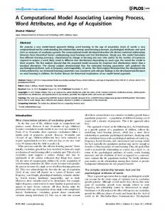
Sensemaking in a hurricane prediction task In cue-learning and categorization literature, many similar paradigms have been used to examine how people predict outcomes based on probabilistic signals. One prominent paradigm is the weather prediction task (WPT) which has been used extensively by Gluck and colleagues (Gluck & Bower, 1988; Knowlton et al., 1994; Gluck et al., 2002) to study learning of probabilistic outcomes (sunny or cloudy) based on a sets of otherwise meaningless cues. Results in such tasks reveal learning trajectories, and also different strategies used (such as considering just the best feature, weighing all features, or considering only positive or negative features, see Gluck et al., 2002). The cognition involved in true weather forecasting is much more complex (see Hoffman, 2017), but at its core weather prediction spans both laboratory and naturalistic contexts, and so is a reasonable testing ground for understanding sensemaking. We have designed a testing system that is similar to the WPT, with a few exceptions that make it more amenable to studying sensemaking, implemented via the cross-platform experiment-design system PEBL (Mueller & Piper, 2014). Describing the general task, (see Figure 1), participants are
first given a description of a set of eight features that serve as predictors of the risk of a hurricane (bottom left panel). One each trial, they are shown a sensor report describing the state of between 0 and 8 weather variables (top panel), that include status of wind, rain, sea level, and the like. They are told that these indicators have strengths between very good and none, and in truth they combine in a logistic model to predict the probability of a hurricane with feature weights .8, .8, .6, .5, .5, .2, .1, and .01. Next, participants are asked to estimate the probability of a hurricane occurring (bottom right panel), and given feedback, awarding points if their estimate was within 7.5% of the true probability. On some trials, correct feedback was given, but on the rest of the trials, erroneous feedback is given, inducing a true or simulated error. When an error was induced or committed, the participant was then asked whether they felt the system was to blame, or they themselves were. This error detection is a simple way of determining whether their knowledge, as they may be correct even when they guess, but may not be able to determine if an error was produced by the system. This mode of operation also mimics many behaviors of humans operating intelligent systems–they need to trust the system, and their ability to predict the system can help produce trust. Overall, we conceive of the task as having the participant learn a forecasting model, rather than learning the weather–they are told that a computer model is creating the prediction that they are trying to match. The underlying model is a logistic regression model, with different independent features having different weights. This task involves several opportunities to examine complementary aspects of sensemaking. These include: • The ability to use instruction to start with a reasonable frame for making a probability prediction • The ability to use feedback to learn how to combine evidence to make a prediction. • the ability to identify the source of errors (themselves or a computer model). In subsequent and prior studies not discussed here, we have also examined other aspects of sensemaking processes and representations, making evacuation decisions, learning nonindependent features, diagnosing sensor errors, and correcting the system to match a given output. Our goal is to use this task to (1) test whether different sensemaking functions rely on a common mental model or knowledge base; and (2) identify possible sources for this knowledge in a computational model that might explain individual differences in performance.
Method All methods were approved by the MTU institutional review board (IRB). We tested 27 participants who took part in the study in exchange for course credit. Participants were first instructed in the task, given several practice trials, and then allowed to move on to the testing phase. They completed a total of 80 trials, which involved combinations of up to 8 features. On each trial, they first made a probability estimate. Next,
Figure 1: Elements of hurricane prediction experiment. Top panel shows typical message. Bottom left shows feature description, and bottom right shows likelihood assessment scale.
the system determined whether an error would be signaled. Errors were signaled whenever the participant made a true error, and on half of all other trials. On system-correct trials, the true probability of the model was shown; on system-error trials a new probability was sampled that was outside a 7.5% region around the true estimate. Participants were asked to determine whether the error came because of themselves (“I was to blame”) or if they thought the system made an error (“the system was to blame”). All participants experienced the same 80 trials, but in a randomized order, and the trials were sampled to produce a range of probability estimates. Once they completed the task, they were debriefed and given credit for completing the study.
Results We first would like to establish that performance differs across individuals. Figure 2 shows scatterplots of the givento-estimated probability across all individuals. The correlations ranged from -.08 to .86, with substantial variability. Our main hypothesis in this study is that the ability to estimate the probability will have related effects in other sensemaking functions, and so we would expect this correlation to predict other behaviors. An ANOVA model incorporating participant code and trial pattern on prediction error showed that participant code was highly significant (F(26, 1996) = 14.3, p < .001), suggesting that substantial systematic variability stems from individual differences. As an alternate measure of individual accuracy, we computed the proportion of trials on which a participant was within 7.5 % of the true model value (which is the criterion for being awarded points). These values are seen in Figure 3, arranged by three error conditions, depending on whether the system or the human was correct. The horizontal axis of Figure 3 shows that the range of abilities in estimation have an impact on blame assessment. The leftmost panel shows that all participants–regardless of
Figure 2: Performance across individuals ranged from close to random (participant 109; R=-.08) to very precise (participant 202; R=.86). 101
102
103
104
105
106
1.00 0.75 0.50 0.25 0.00
● ●● ● ● ●●●●●● ● ●●● ●● ● ●● ●● ● ● ● ●● ● ● ●● ●● ● ● ● ● ● ●● ●●●●●● ● ● ●● ● ● ● ● ●● ● ● ●● ● ●
● ● ● ●●●● ● ● ● ●● ●●●●● ● ● ● ● ●●● ●● ● ● ●● ● ●● ●● ● ●● ● ● ● ● ●● ●● ● ●● ● ● ● ●● ● ● ●● ● ● ● ● ● ●● ● ● ● ●
●●●● ● ● ●●●● ● ● ● ●●●●●●● ●● ● ●● ● ●● ● ● ● ●● ●● ● ● ●● ● ● ● ● ●● ●●●● ● ● ●● ●●● ● ● ●●●●●●●● ● ● ● ●● ●
● ● ●●●● ● ● ●●● ● ●● ● ● ●●●●●● ●● ●●● ●● ●●●● ●● ●● ● ●● ● ● ●●●● ● ● ●● ● ● ●●● ● ● ●
● ●● ● ● ● ● ● ●● ●● ● ●● ● ● ● ● ● ● ● ●● ● ●●●●● ●●●● ● ● ●● ● ●●●● ● ● ●●●●●●● ●● ●● ● ● ●●● ● ●● ●● ● ●
● ●● ● ●● ● ●● ● ● ● ●●● ●● ● ● ●● ● ● ● ● ● ●●● ● ● ●●● ●●●●● ● ● ● ● ● ● ●● ●● ● ● ● ●●● ● ● ●● ●● ● ● ● ● ● ● ●● ●●
108
109
1.00 0.75 0.50 0.25 0.00
● ● ● ●● ● ● ● ● ● ● ● ● ●● ● ●● ● ●●● ● ●● ●● ● ● ● ● ●● ● ●●●●●● ● ●● ●● ● ●● ●● ● ● ●● ●●● ●● ● ● ●● ● ●● ●● ● ●
163
200
201
202
1.00 0.75 0.50 0.25 0.00
● ● ●●●●● ● ● ●●●● ●● ● ● ● ●●●● ●●●● ● ●● ●●●● ●● ●●● ●●● ● ● ●● ●● ● ●● ●● ● ● ● ●● ● ● ●
● ● ● ● ● ● ● ● ●●●●● ● ●●●● ● ●● ●●● ● ●●● ●● ●● ●●● ●● ● ●● ●● ● ● ● ● ● ●●● ● ●● ● ● ●●● ● ● ●●● ● ●●● ● ●
● ● ● ● ● ● ● ●● ●● ● ●●● ●●● ● ●●● ●● ● ●● ●● ● ●● ●● ● ● ●●●●● ●● ● ●●●● ● ● ●● ● ●●●●● ●● ● ●● ●● ● ● ● ●●
● ● ●● ● ●● ●●● ●● ● ●● ● ● ● ●● ● ●● ●●●● ●●● ● ● ●●●●●● ● ● ● ● ●●● ● ● ●● ● ● ● ●●●● ● ●
205
206
207
208
209
270
●● ● ● ● ●● ●●● ● ●● ● ●●●● ● ● ● ● ● ● ● ● ● ●●●● ● ●● ●● ●● ●● ● ●●● ● ● ●●● ● ● ●●●● ● ● ●● ● ● ●● ● ●●
● ● ● ●● ● ● ● ● ●●● ●● ●●●● ● ● ●●●● ●●● ● ● ● ● ● ● ● ●● ● ●● ● ●● ● ● ● ●●● ● ● ● ●● ● ● ● ● ●●● ● ●●●●● ● ●
●● ● ● ● ●● ●● ● ● ● ● ●●●●● ● ●●●●● ● ●●● ● ● ● ● ●● ● ● ●● ● ● ● ● ● ● ● ● ● ●● ●●● ● ●● ●●●● ●● ● ●● ● ●● ●●●
● ● ● ● ●● ●● ● ●● ●● ●● ● ●● ●● ● ●● ●● ● ● ● ● ● ●● ● ● ●●● ●● ● ● ● ● ●● ●● ●● ●● ● ●●●●● ●● ● ●● ●● ● ● ●●●
● ● ● ● ● ● ● ●● ●● ●●●● ● ● ●● ●●●●● ● ● ●● ● ● ● ● ● ●●●●● ● ● ● ● ● ● ●● ●● ● ●●● ● ● ● ● ● ● ● ●● ● ● ●● ● ●● ●● ●●
● ● ● ●●● ● ●●● ●● ● ●●● ●● ●●●●● ● ● ●●● ●●●● ● ● ●● ●● ● ● ● ● ●● ● ●●● ●● ● ● ● ● ●●● ● ● ●
0.250.500.75
0.250.500.75
0.250.500.75
●
clickval
107
1.00 0.75 0.50 0.25 0.00 1.00 0.75 0.50 0.25 0.00
● ● ● ● ● ● ●● ●● ● ●●● ● ●● ● ● ● ● ● ● ● ● ●● ●● ●●●● ● ●● ● ●● ● ● ●● ● ●●●● ●● ● ● ● ● ●●●● ● ●● ● ● ●● ●●● ● ●
●
●
160
161
162
● ●● ●● ● ● ● ● ● ●●● ●● ● ● ● ● ● ●●●●●● ● ●● ●●● ● ●● ● ● ● ● ● ● ● ●●●● ● ●● ● ●● ● ●●●● ● ●
● ●●● ● ●● ● ● ● ●● ● ● ●● ●●● ● ●● ● ● ● ● ● ● ● ● ●●●● ●●●● ● ● ● ● ● ● ● ●● ● ●● ● ● ●●●● ● ●● ● ● ● ●● ● ●●●● ●●● ●
● ●● ●● ● ●●●● ● ●●● ●● ●●● ● ● ● ● ● ● ●● ●● ●● ●●●● ● ● ● ●● ● ● ● ●●● ●●●●●●●●● ● ● ● ●●●● ● ● ● ● ● ●●
●●
● ● ● ●● ● ● ●●● ● ● ●● ● ●●● ●● ●●● ●● ●● ● ●● ●●●● ●● ●●● ● ●●●● ●●●●●●●●● ● ● ● ● ●
271
272
273
● ● ●●● ●● ●● ●●● ● ● ● ● ● ● ● ● ●● ● ● ● ● ●●
● ● ● ● ●● ● ● ● ● ●●●●● ●●●● ●● ● ●●● ●●●● ● ●●● ● ● ● ●●● ●●●● ●●● ● ●●●● ● ● ● ●● ●●● ● ● ● ● ● ● ● ●
● ● ● ● ●● ● ● ● ●● ● ● ●● ● ● ●● ● ● ● ● ● ●●●● ● ●●● ● ● ●● ● ●●● ● ●● ● ● ●●● ●● ●●● ● ● ● ● ●●●●●●●●● ●●● ● ● ● ●
0.250.500.75
0.250.500.75
0.250.500.75
● ●● ● ●● ● ●●
203 ●● ● ●●●● ●● ● ●●● ● ●●●●● ●●●● ● ● ● ●●● ● ● ●●●●● ● ●● ●● ● ● ● ● ● ● ● ● ●●●● ●● ● ● ● ●● ● ●● ●●●●● ● ●
204 ●● ● ●● ●● ●●● ● ● ● ● ●● ● ● ●●●●●●● ●● ● ● ● ●● ●● ●● ● ● ● ●●●● ● ● ● ● ● ●● ● ● ●● ● ● ●●●●● ●● ●
a similar context many participants considered only the best features, but others considered more. Our own intuition is that we perform some intuitive mental arithmetic: starting at a baseline value (e.g., 50%) and adjusting the probability higher and lower based on the presence of positive and negative features, assuring to give the stronger indicators more weight and not permit probabilities to extend outside the 0100% range. In post-experiment interviews, we have found that participants have sometimes reported strategies like this, but they also indicate many misconceptions, including setting a baseline that is not 50%. So, our initial model assumes that for each predictor, people understand its relative weight in predicting a probability of a storm, these weights add together to form an internal odds ratio, which is transformed to a probability using a logit transform logistic(x) = 1/(1 + e−x ). This is identical to the logistic regression model without error: p = logistic(∑ fi βi )
●
trueprob
how well they estimate probability, tend to blame themselves when the system was correct but an error was made. The rightmost panel shows what happens when the person is actually correct but the system is incorrect. Here, those who do worse also tend to blame themselves. In contrast, those who do better tend to blame the system. In this case, blaming the system is the “correct” response, and we see that those who are better at estimating the probability are better at assessing blame for errors. The center panel shows what happens when both the human and computer are wrong, and the results do not differ substantially from the rightmost panel. This result demonstrates that ability to estimate the probability is useful for detecting an error and appropriately assigning blame– suggesting that an emergent process is involved.
A Computational Model of Sensemaking We have designed the experiment so that the mental model of performance is fairly simple, and maps onto a simple linear model with a logistic transform. More complex mental models may require networks or hierarchies of such models, but at its core the notion is akin to modeling estimation with an improper linear model (Dawes, 1979). This is a generalization of the framework was used by Mueller (2009) to implement a core Recognition-primed decision process.
Probability Prediction The first function to consider is how a probability estimate is made when a set of features is shown. There are numerous theories about how people make estimates in light of complex probabilistic data. Gluck et al., (2002) argued that in
(1)
i
Here, fi are feature values that are either +1 (consistent with hurricane), -1 (consistent with calm), or 0 (absent). The coefficients βi can differ for each predictor, but in our initial model, all features that are present are used, and a probability is estimated exactly from the beta weights and feature values, with no error. If an individual has a good intuitive estimate of the βi values, they should be able to produce a close approximation to the true probability; otherwise, they are likely to mis-estimate the probability.
Learning rule . Next, we must consider how the βi weights change over time. Many learning schemes are based on the so-called ‘delta’ rule: if a feature is present and its value is positive, errors between the model and the feedback signal should adjust the beta weights to reduce the likelihood of future error (see Rescorla & Wagner, 1972; Gluck & Bower, 1988). If the message contains features fi ∈ −1, 0, 1, the weights at time j [ j] are βi , the difference between the estimated probability and the feedback is ε, and α is a learning rate parameter, [ j+1]
βi
[ j]
= βi + ε ∗ (1 − fi ) ∗ | fi | ∗ α
(2)
The inner 1 − fi implicitly assumes that the canonical pattern for maximum chance of a hurricane is all features set to 1.0. For more complex classification schemes in which different classification patterns are of interest, this could be replaced with pi − fi , where pi is a prototype classification pattern. The logic of the learning rule is that β values are changed from previous values in the direction that would reduce error, but only for the features that are present (-1 or 1).
Error and Anomaly Detection As currently described, it is not clear how an error could reasonably assessed. This is in part because the model has no
Figure 3: Results from weather sensemaking experiment. Individuals who are better at estimating the model’s probability are also better at discriminating correct model behavior (left panel) from incorrect model behavior (center and right panels).
0.0
0.2
0.4
0.6
0.8
Proportion within 7.5%
1.0
1.0
●worse ● 0.0
0.2
0.4
0.8
●
0.8
1.0
Proportion within 7.5%
sense of how sure it is about its β values. For any set of features, it can provide an estimate, but this estimate will almost never be exactly the same as the true model prediction. Thus, we need to consider how the model knows the value is likely to have arisen from its internal model. Clearly, a number of mechanisms could suffice. A simple bounded confidence model would identify any estimates greater than some fixed difference as outside the model’s bounds, but Mueller and Tan (2017) questioned the utility of such models in many contexts. Many likelihood-based model and fuzzy models could have the ability to provide bounds on the outcome estimates. For example, if the β weights were not point estimates but rather distributions, the posterior estimate would also be a distribution, and the likelihood of that distribution could be measured by applying Bayes rule–and in fact the β weights could be estimated via Bayesian inference. We have opted for an approach that approximates this, without requiring the mechanisms and distributional assumptions of Bayesian inference. We assume that instead of a single set of beta weights, the individual has a collection of independent prediction models whose coefficients start randomly and evolve independently over time. One might consider the multiple versions of each parameter an empirical prior distribution, or a fuzzy-set representation of the uncertainty in the value. For example, an agent may have have ten versions of beta estimates. On each trial, a prediction can be made by sampling one or more of these versions and using it to compute estimates. This provides both a noisy estimation, and the possibility of using mental simulation to sample a range of possible values. When feedback is given, a subset of the models (as few as 1, but multiple are possible) are sampled and updated using Equation 2. Models thus can start out with a wide range of values, producing a range of possible outcomes, but over time will converge to similar weights and similar predictions. Thus an agent that has multiple sets that
0.6
● ●●
●● ● ● ● ● ● ● ● ●
0.2
better
0.6
● ●
0.4
● ● ●● ● ● ● ●● ●
0.0
0.0
●
● ●
● ● ● ● ●● ● ●
0.2
0.4
● ● ●
●● ●●●●
worse
0.0
0.6
●● ●
System Incorrect Human Correct
Proportion blaming self
1.0 0.8
● ●
● ● ● ● ● ●
0.6
● Proportion blaming self
0.8
●●● ● ●● ● ● ● ● ● ● ● ● ● ●
0.2
Proportion blaming self
System Incorrect Human Error
0.4
1.0
System Correct Human Error
● 0.0
0.2
0.4
●● better
0.6
0.8
1.0
Proportion within 7.5%
are similar can be highly confident in its estimate (even if it is not calibrated), whereas an agent with very different weights will have less confidence in its estimate. This scheme has a direct functionality for blame assessment. An agent can make an estimate by sampling one model and producing an estimate. But if the agent is given another estimate, it can estimate the likelihood that the estimate arose from any of its models. Although this posterior distribution could be generated by smoothing or estimating a specific distribution, we will use the simple decision policy of asking whether the given estimate is outside the entire range of estimates the agent could make at any point in time. An estimate outside the set of possible estimates is considered anomalous or an error. In the current design, detecting an error is synomomous with assigning blame. That is, if the given feedback is outside of the agent’s bounds, it is judged as being the fault of the system, rather than the agent. Thus, agents with β weights that are similar will be likely to detect that the system is broken even when the amount of error is small, but agents with widely varied weights are likely to produce an estimate even more extreme than the error, and thus attribute the error to their own lack of knowledge.
Simulation The behavioral data showed systematic differences in how accurate people were in estimating the probability. There are multiple ways in which we might represent individual differences in ability in the model. Two natural explanations are that (1) there are differences in how well people learn in response to feedback; and (2) there are differences in how well people generate initial (prior) estimates of β weights in response to instructions. There are other possibilities as well, such as how many versions of the β weights are stored, how many are update in response to a given piece of feedback, and
0.20
0.30
1.0 0.8 0.10
0.30
0.05
Pr(Blame oneself)
0.8 0.6
2.0
0.2 0.0
0.2 0.0 1.5
0.35
Proportion within 7.5%
0.4
Pr(Blame oneself) 1.0
Priors Std. Dev.
0.25
0.8
0.6 0.5 0.4 0.3 0.2 0.0
0.5
0.15
1.0
Learning rate
0.1
Proportion within 7.5%
0.20
1.0
Learning rate
0.0
0.6 0.2 0.0
0.00
0.6
0.10
0.4
0.00
0.4
Pr(Blame oneself)
0.8 0.6 0.0
0.2
0.4
Pr(Blame oneself)
0.25 0.15 0.05
Proportion within 7.5%
0.35
1.0
Figure 4: Results from two simulations (n=5000). Left panels show how prediction error is impacted by varying either learning rate (top panel) or prior noisy (bottom panel). Center panels show impact of learning rate on probability of blaming oneself either when the system is correct (black) or incorrect (gold). Right panels show relationship between prediction accuracy and blame, analogous to data in Figure 2. Dashed lines represent best-fit linear-model for simulation, and solid lines represent best-fit linear model from human data in Figure 2.
0.0
0.5
1.0
1.5
Priors Std. Dev.
the extent to which multiple versions might be sampled prior to making an estimate. To examine how this model can account for results of the experiment, we conducted two simulation studies. In each study, we had each agent go through the 80-trial design that human subjects were exposed to, making an estimate, getting feedback, and assigning blame on each trial. For each of 5000 simulated participants, we recorded their accuracy across the 80 trials (in terms of the proportion of trials within 7.5% of the true value), and their blame assessment probabilities for both system correct and incorrect trials (mapping onto the left and right panels of Figure 3). In all models, agents initiated an ensemble of 8 beta-weight sets, and on each update, four sets were sampled (with replacement) and a single delta-rule step was initiated on each. These simulations have no free parameters for fitting the human data in Figure 3, and the only arbitrary parameters involve the number of beta-weight
2.0
0.0
0.1
0.2
0.3
0.4
0.5
0.6
Proportion within 7.5%
ensembles, the number of ensembles sampled on each set, along with the prior distribution in Simulation 1 (set to a uniform distribution between 0 and 2) and the learning rate in Simulation 2 (set to 0). The top panel of Figure 4 shows simulation results for a model in which the main between-agent variable was the learning rate. On each simulation, a learning rate parameter was sampled between 0.0 and 0.3 (horizontal axis of left panel of Figure 4). As learning rate increased, overall accuracy increased (note that as seen in Figure 3, typical values produced by human participants ranged from about .2 to .6). As learning rate gets larger, we see that the ability to discriminate system-correct errors (black points) from system-incorrect errors (gold points) increases. The right panel shows a plot akin to that in Figure 3. Overall, the system-error trials show very similar results to the human data. In contrast, the systemincorrect condition shows a negative slop (like human data
did), but there are some overall mismatches. Nevertheless, the qualative pattern is similar, suggesting that a learning-rate account may explain the individual differences we found. The bottom panel of Figure 4 shows a model that involves no learning (α = 0.0), but systematically varies the standard deviation of the different examplars of each β weight around a starting level that matched the true model (.8, .8, .6, .5, .5, .2, .1, and .01). The rightmost panel shows that as the standard deviation of the values increased, overall accuracy decreased, and when the standard deviation was near 0, performance was close to 50% (half of trials were estimated within 7.5% of the true value). Now, when comparing performance to blame assessment, the slope of the system-incorrect trials (in gold) is perhaps a better approximation of the human data. The main problem is that when the system is correct, the agent correctly blames the system close to 100% of the time, in contrast to humans who blame the system around 80% of the time. This difference likely arises because the starting values were centered on the true values, and so the correct estimate would almost always be in the center of the estimates. Had the starting mean beta weights been less calibrated, more correct estimates would have been outside the agents estimates and this probability would have been lower.
Discussion The two simulations provide two examples of model parameters that might produce the systematic variability we saw in our human experiments. Each produced some mismatches to data, but they are nevertheless informative about what kinds of individual differences may produce systematic differences in sensemaking ability. We find the model involving better assessment of priors more satisfying in its account of our data, aside from it being too good when it made an error. To examine the difference between these in greater detail, we fit a linear regression model predicting overall error rate by participant and trial, and also computed accuracy across the entire experiment and for the first five trials. We found that the accuracy for the first five trials was highly correlated with the performance over the entire task (R = .79, t = 6.4, p < .001). Performance on the first five trials was negatively correlated with slope (R = −.41, t = 2.23, p = .03), but performance over the entire experiment was not (R = −.15, t = .76, p = .45). The negative slopes indicate that people who had less error at the beginning overall had relatively more positive slopes. In other words, those who started out good improved less than those who started out more poorly. This suggests that both of the factors studied in the simulation may be at play. Some people are able to set good priors, and so if they are, they are good immediately and end up doing the best of all participants. Others start out less good, and tend to improve more, but their overall performance remains worse than those who start off good.
Conclusions This model attempts to integrate several complementary functions related to sensemaking that have previously been stud-
ied mainly in isolation. We found that performance in one skill (estimation) is predictive of performance in a second task (assessing whether an error arose because of the person or the system). Our computational model of sensemaking integrates different functions via a simple model, and incorporates error detection by assuming that feature-weights are fuzzy and encoded as an ensemble of values that get updated independently. This type of assumption is not necessary when studying just the learning aspect of the task, but by adding additional sensemaking tasks, we are able to identify, simulate, and discriminate sources of individual differences, which involve both ability to set reasonable feature-weight estimates based on instruction, and ability to learn based on trial-bytrial feedback.
Acknowledgments The experiment presented in this paper was part of the Master’s thesis of BN. The modeling was supported by DARPA Explainable Artificial Intelligence (XAI) program.
References Dawes, R. M. (1979). The robust beauty of improper linear models in decision making. American psychologist, 34(7), 571–582. Gluck, M. A., & Bower, G. H. (1988). From conditioning to category learning: An adaptive network model. Journal of Experimental Psychology: General, 117(3), 227–247. Gluck, M. A., Shohamy, D., & Myers, C. (2002). How do people solve the “weather prediction” task?: Individual variability in strategies for probabilistic category learning. Learning & Memory, 9(6), 408–418. Hoffman, R. R., LaDue, D. S., Trafton, J. G., Mogil, H. M., & Roebber, P. J. (2017). Minding the weather: How expert forecasters think. MIT Press. Knowlton, B. J., Squire, L. R., & Gluck, M. A. (1994). Probabilistic classification learning in amnesia. Learning & Memory, 1(2), 106–120. Klein, G., Moon, B., & Hoffman, R. R. (2006). Making sense of sensemaking 1: Alternative perspectives. IEEE intelligent systems, 21(4), 70–73. Klein, G., Moon, B., & Hoffman, R. R. (2006). Making sense of sensemaking 2: A macrocognitive model. IEEE Intelligent systems, 21(5), 88–92. Mueller, S. T. (2009). A Bayesian recognitional decision model. Journal of Cognitive Engineering and Decision Making, 3(2), 111–130. Mueller, S. T., & Piper, B. J. (2014). The psychology experiment building language (PEBL) and PEBL test battery. Journal of neuroscience methods, 222, 250-259. Rescorla, R. A., & Wagner, A. R. (1972). A theory of Pavlovian conditioning: Variations in the effectiveness of reinforcement and nonreinforcement. Classical conditioning II: Current research and theory, 2, 64–99.