A Computational Model of Time-Dilation

A Computational Model of Time-Dilation Charles Davi March 20, 2018 Abstract We propose a model of time-dilation that follows from the application of concepts from information theory and computer theory to physical systems. Our model predicts equations for time-dilation that are identical in form to those predicted by the special theory of relativity, except in one case. In that one case, the actual numerical di↵erences between the results predicted by our model and those predicted by the special theory of relativity are extremely small, and thus, our model is consistent with existing experimental tests of time-dilation. In short, our model can be viewed as an alternative set of postulates rooted in information theory and computer theory that imply that time-dilation will occur.

1

Introduction

Prior to the twentieth century, physicists appear to have approached nature with a general presumption that fundamental physical properites such as energy and charge are continuous. This was likely the result of a combination of prevailing philosphocial views, and mathematical convenience, given that continuous functions are generally easier to calculate than discrete functions. However, this view of nature began to unravel in the early twentieth century as a result of the experiments of Robert A. Millikan, and others, who demonstrated that charge appeared to be an integer multiple of a single value, the elementary charge e [15], and confirmed Einstein’s predictions for the energy of electrons ejected due to the photoelectric e↵ect, which suggested a quantized, particle theory of light [16]. In the century that followed these experiments, the remarkable success of quantum mechanics as a general matter demonstrated that whether or not the ultimate, underlying properties of nature are in fact discrete, the behavior of nature can nonetheless be predicted to a high degree of precision using models that make use of discrete values. This historical progression from a presumption of continuous values, towards the realization that fundamental properties of nature such as charge are quantized, was facilitated in part by the development of experimental techniques that were able to make measurements at increasingly smaller scales, and the computational power of the computer itself, which facilitated the use of discrete calculations that would be impossible to accomplish by hand. Though admittedly anecdotal, this progression suggests the 1

possibility that at a sufficiently small scale of investigation, perhaps we would find that all properties of nature are in fact discrete, and thus, all apparently continuous phenomena are simply the result of scale. Below we show that if we assume that all natural phenomena are both discrete, and capable of being described by computable functions, then we can achieve a computational model of time-dilation that predicts equations that are generally identical in form to those predicted by the special theory of relativity.

1.1

The Information Entropy

Assume that the distribution of characters in a string x is {p1 , . . . , pn }, where pi is the number of instances of the i-th character in some alphabet ⌃ = {a1 , . . . , an }, divided by the length of x. For example, if x = (ab), then our alphabet is ⌃ = {a, b}, and p1 = p2 = 12 , whereas if x = (aaab), then p1 = 34 and p2 = 14 . The minimum average number of bits per character required to encode x as a binary string without loss of information, taking into account only the distribution of characters within x, is given by, H(x) =

n X

pi log(pi ).1

(1)

i=1

We call H(x) the information entropy of x. The intuition underlying the information entropy is straightforward, though the derivation of equation (1) is far from obvious, and is in fact considered the seminal result of information theory, first published by Claude Shannon in 1948 [17]. To establish an intuition, consider the second string x = (aaab), and assume that we want to encode x as a binary string. We would therefore need to assign a binary code to each of a and b. Since a appears more often than b, if we want to minimize the length of our encoding of x, then we should assign a shorter code to a than we do to b. For example, if we signify the end of a binary code with a 1, we could assign the code 1 to a, and 01 to b.2 As such, our encoding of x would be 11101, and since x contains 4 characters, the average number of bits per character in our encoding of x is 54 . Now consider the first string x = (ab). In this case, there are no opportunities for this type of compression because all characters appear an equal number of times. The same would be true of x = (abcbca), or x = (qs441z1zsq), each of which has a uniform distribution of characters. In short, we can take advantage of the statistical structure of a string, assigning longer codes to characters that appear less often, and shorter 1 All

lograthims referenced in this paper are base 2. than make use of a special delimiting character to signify the end of a binary string, we could instead make use of a“prefix-code”. A prefix code is an encoding with the property that no code is a prefix of any other code within the encoding. For example, if we use the code 01 in a given prefix code, then we cannot use the code 010, since 01 is a prefix of 010. By limiting our encoding in this manner, upon reading the code 01, we would know that we have read a complete code that corresponds to some number or character. In contrast, if we include both 01 and 010 in our encoding, then upon reading an 01, it would not be clear whether we have read a complete code, or the first 2 bits of 010. 2 Rather

2

codes to characters that appear more often. If all characters appear an equal number of times, then there are no opportunities for this type of compression. In general, if a string x is drawn from an alphabet with n characters, and the distribution of these characters within x is uniform, then H(x) = log(n), which is the maximum value of H(x) for a string of any length drawn from an alphabet with n characters. Shannon showed in [17] that a minimum encoding of x would asign a code of length li = log( p1i ) to each ai 2 ⌃. If the length of x is N , then each ai will appear N pi times within x. Thus, the minimum total number of bits required Pn to encode x using this type of statistical compression is i=1 N pi li = N H(x). Therefore, the minimum average number of bits per character required to encode a string of length N is H(x). Note that H(x) is not merely a theoretical measure of information content, since there is always an actual binary encoding of x for which the average number of bits per character is approximately H(x) [12]. Thus, H(x) is a measure of the average number of bits required to actually store or transmit a single character in x. However, the value of H(x) is a function of only the distribution of characters within x, and therefore, does not take into account other opportunities for compression. For example, a string of the form x = aN bN cN has an obvious structure, yet H(x) = log(3) is maximized, since x has a uniform distribution of characters. Thus, even if a string has a high information entropy, the string could nonetheless have a simple structure.

1.2

The Information Content of a System

Despite the limitations of H(x), we can still use H(x) to measure the information content of representations of physical systems, understanding that we are able to account for only the statistical structure of the representation. We begin with a very simple example: consider a system comprised of N particles that initially all travel in the same direction, but that over time have increasingly random, divergent motions. We could represent the direction of motion of each particle relative to some fixed axis using an angle ✓. If we fix the level of detail of our representation of this system by breaking ✓ into groups of A = [0, ⇡2 ), B = [ ⇡2 , ⇡), 3⇡ C = [⇡, 3⇡ 2 ), and D = [ 2 , 2⇡), then we could represent the direction of motion of each particle in the system at a given moment in time as a character from ⌃ = {A, B, C, D} (see Figure 1 below). Note that this is clearly not a complete and accurate representation of the particles, since we have, for example, ignored the magnitude of the velocity of each particle. Nonetheless, we can represent the direction of motion of all of the particles at a given moment in time as a string of characters drawn from ⌃ of length N . For example, if at time t the direction of motion of each particle is ✓ = 0, then we could represent the motions of the particles at t as the string x = (A · · · A), where |x| = N . As such, the distribution of motion is initially entirely concentrated in group A, and the resultant distribution of characters within x is {1, 0, 0, 0}. The information P4 3 entropy of {1, 0, 0, 0} is i=1 pi log(pi ) = 0 bits, and therefore, the minimum 3 As

is typical when calculating H(x), we assume that 0 log(0) = 0.

3

average number of bits per character required to encode this representation of the particles at t is 0 bits. Over time, the particles will have increasingly divergent motions, and as such, the distribution of characters within x will approach the uniform distribution, which is in this case { 14 , 14 , 14 , 14 }, which has an information entropy of log(4) = 2 bits. Thus, the information entropy of this representation of the particles will increase over time. ⇡ 2

✓!A

⇡

0

3⇡ 2

Figure 1: A mapping of angles to ⌃ = {A, B, C, D}. We could argue that, as a result, the information content of the system itself increases over time, but this argument is imprecise, since this particular measure of information content is a function of the chosen representation, even though the behavior of the system can impact the information content of the representation. For example, if we made use of a finer gradation of the angle ✓ above, increasing the number of groups, we would increase the number of characters in our alphabet, thereby increasing the maximum information content of the representation, without changing the system in any way. However, this does not imply that representations are always arbitrary. For example, if some property of a system can take on only n discrete values, then a representation of the system that restricts the value of this property to one of these n values is not arbitrary. The point is that as a practical matter, our selection of certain properties will almost certainly be incomplete, and measured at some arbitrary level of precision, which will result in an arbitrary amount of information. Thus, as a practical matter, we probably cannot answer the question of how much information is required to completely and accurately represent a physical system. We can, however, make certain assumptions that would allow us to construct a complete and accurate representation of a system. Assumption 1.1. There is a finite set of n measurable properties such that (1) for any measurable property P 62 , the value of P can be derived from the 4

values of the properties Pi 2 , and (2) there is no Pi 2 of Pi can be derived from the other n 1 properties in

such that the value Pi .

We call each of the properties Pi 2 a basis property. Note that we are not suggesting that all properties are a linear combination of the basis properties within . Rather, as discussed in Sections 1.3 and 2 below, we assume that all other measurable properties can be derived from using computable functions. For example, if mass and velocity are included in , then Assumption 1.1 implies that momentum would not be included in , since momentum can be derived from mass and velocity using a computable function.4 Assumption 1.2. For any closed system,5 each Pi 2 finite number of possible values.

can take on only a

For example, assume that a closed system S contains a finite number of N elements.6 Assumption 1.1 implies that there is a single set of basis properties from which all other measurable properties of any given element can be derived. As such, in this case, S consists of a finite number of elements, each with a finite number of measurable basis properties, and Assumption 1.2 implies that each such basis property can take on only a finite number of possible values. Assumption 1.3. For any system, all measurable properties of the system, as of a given moment in time, can be derived from the values of the basis properties of the elements of the system, as of that moment in time. Together, Assumptions 1.1, 1.2, and 1.3 allow us to construct a complete and accurate representation of a system at a given moment in time. Specifically, if we were able to measure the basis properties of every element of S at time t, then we could construct a representation of the state of S as a set of N strings S(t) = {s1 , . . . , sN }, with each string representing an element of S, where each string si = (v1 , . . . , vn ) consists of n values, with vj representing the value of the j-th basis property of the i-th element of S at time t. Because S(t) contains the values of the basis properties of every element of S at time t, Assumption 1.3 implies that we can derive the value of any property of S at time t from the representation S(t) itself. For example, Assumption 1.3 implies that there is some computable function f that can calculate the momentum ⇢ of S at time t when given S(t) as input. Expressed symbolically, ⇢ = f (S(t)). Thus, S(t) contains all of the information necessary to calculate any measurable property of S at time t, and therefore, we can take the view that S(t) constitutes a complete and accurate representation of the state of S at time t. Note that Assumption 1.3 does not imply that we can determine all future properties of S given the values of the basis properties of its elements at time t, but rather, that the value 4 We

will discuss computable functions in greater detail in Sections 1.3 and 2 below, but for now, a computable function can be defined informally as any function that can be implemented using an algorithm. 5 We view a system as closed if it does not interact with any other systems or exogenous forces, and is bounded within some definite volume. 6 We deliberately use the generic term “element”, which we will clarify in Section 2 below.

5

of any property of S that exists at time t can be derived from the values of the basis properties of its elements as of time t.7 Of course, we are not suggesting that we can construct such a representation as a practical matter, but rather, we will use the concept of S(t) as a theoretical tool to analyze the information content of systems generally, and ultimately, construct a model of time-dilation. Recall that Assumption 1.2 implies that each basis property of S can take on only a finite number of possible values. If we assume that the n basis properties are independent, and that basis property Pi can take on ki possible values, then the basis properties of each element of S can have any one of K = k1 · · · kn possible combinations of values. If we distinguish between the N elements of S, and assume that the basis properties of each element are independent from those of the other elements, then there are K N possible combinations of values for the basis properties of every element of S. Since the values of the basis properties of the elements of S determine all measurable properties of S, it follows that any definition of the overall state of S will reference either the basis properties of the elements of S, or measurements derived from the basis properties of the elements of S. As such, any definition of the overall state of S will ultimately reference a particular combination of values for the basis properties of the elements of S. For example, Assumption 1.3 implies that the temperature of a system is determined by the values of the basis properties of its elements. Therefore, the maximum number of states of S is equal to the number of unique combinations of values for the basis properties of the elements of S, regardless of our choice of the definition of the overall state of S.8 We can assign each such state a number from 1 to K N , and by Si we denote a representation of the i-th state of S. That is, S(t) denotes a representation of the state of S at time t, whereas Si denotes a representation of the i-th possible state of S in some arbitrary ordering of the states of S. Thus, for any given moment in time t, there exists an Si such that S(t) = Si . By |S| = K N we denote the number of possible states of S. Now imagine that we measure the value of every basis property of every element of S over some long period of time, generating M samples of the state of S, and that for each sample we store the number assigned to the particular state of S we observe. For example, if we observe Sj , then we would add the number j to our string. Thus, in this case, ⌃ = {1, . . . , |S|} is the alphabet, and the resultant string is a string of numbers x = (n1 · · · nM ), representing the M states of S observed over time. Further, assume that we find that the distribution of the states of S over that interval of time is ' = {p1 , . . . , p|S| }, where pi is the number of times Si is observed divided by the number of samples M . We could then encode x as a binary string, and the minimum average number of P|S| bits required to identify a single state of S would be H(x) = i=1 pi log(pi ). Note that we are not encoding the values of the basis properties of the elements within S(t), but we are instead representing each observed state of S with a number, and encoding the resultant string of numbers. That is, each possible 7 We

will discuss calculating future states of systems in Section 1.4 below. will revisit this topic in the context of computable functions on the basis properties of a system in Section 2 below. 8 We

6

combination of values for the basis properties of the elements of S corresponds to a particular unique overall state of S, which, when observed, we represent with a number. In contrast, in Section 1.4 below, we will use the Kolmogorov complexity to measure the information contained in an encoding of S(t) itself. If the distribution ' is stable over time, then we write H(S) to denote the information entropy of x, which we call the representational entropy of S. Thus, H(S) is the average number of bits per state necessary to identify the particular states of S that are observed over time. If ' is the uniform distribution, then we have, H(S) = log(|S|).

(2)

Thus, the representational entropy of a system that is equally likely to be in any one of its possible states is equal to the logarithm of the number of possible states. We note that equation (2) is similar in form to the thermodynamic entropy of a system kB ln(⌦), where kB is the Boltzmann constant, and ⌦ is the number of microstates the system can occupy given its macrostate. This is certainly not a novel observation, and the literature on the connections between information theory and thermodynamic entropy is extensive. (See [2] and [14]). In fact, the similarity between the two equations was noted by Shannon himself in [17]. However, the goal of our model is to achieve time-dilation, and thus, a review of this topic is beyond the scope of this paper. Finally, note that if ' is stable, then we can interpret pi as the probability that S(t) = Si for any given t, and therefore, we can view H(S) as the expected number of bits necessary to identify a single state of S. We can also view S as a medium in which we can store information. The number of bits that can be stored in S is also equal to log(|S|), regardless of the distribution ', which we call the information capacity of S. Under this view, we do not observe S and record its state, but rather, we “write” the current state of S by fixing the value of every basis property of every element of S, and use that state to represent a number or character. As such, when we “read” the current state of S, measuring the value of every basis property of every element of S, we can view each possible current state Si as representing some number or character, including, for example, the number i. As such, S can represent any number from 1 to |S|, and thus, the information contained in the current state of S is equivalent to the information contained in a binary string of length log(|S|).9 For example, whether the system is a single switch that can be in any one of 16 states, or a set of 4 switches that can be in any one of 2 states, in either case, measuring the current state of the system can be viewed as equivalent to reading log(16) = 4 bits of information. Thus, each state of S can be viewed as containing log(|S|) bits of information, which we call the information content of S. Note that the representational entropy of a system is a measure of how much information is necessary to identify the states of a system that are observed over 9 Note that a binary string of length log(|S|) has |S| states, and as such, can code for all numbers from 1 to |S|.

7

time, which, although driven by the behavior of the system, is ultimately a measure of an amount of information that will be stored outside of the system itself. In contrast, the information capacity and information content of a system are measures of the amount of information physically contained within the system. Though the information capacity and the information content are always equal, conceptually, it is worthwhile to distinguish between the two, since the information capacity tells us how much information a system can store as a general matter, whereas the information content tells us how much information is observed when we measure the basis properties of every element of a given state of the system. Finally, note that if a system is closed, then no exogenous information has been “written” into the system. Nonetheless, if we were to “read” the current state of a closed system, we would read log(|S|) bits of information. The information read in that case does not represent some exogenous symbol, but is instead the information that describes the basis properties of the system. Thus, the amount of information observed we measure the basis properties of every element of a given state of the system is log(|S|) bits.

1.3

The Kolmogorov Complexity

Consider again a string of the form x = aN bN cN . As noted above, x has an obvious structure, yet H(x) = log(3), which is the maximum information entropy for a string drawn from an alphabet with 3 characters. Thus, the information entropy is not a measure of randomness, since it can be maximized given strings that are clearly not random in any sense of the word. Assume that N = 108 , and that as such, at least |x|H(x) = 3 ⇥ 108 log(3) bits are required to encode x using a statistical encoding. Because x has such an obvious structure, we can write and store a short program that generates x, which will probably require fewer bits than encoding and storing each character of x. Note that for any given programming language, there will be some shortest program that generates x, even if we can’t prove as a practical matter that a given program is the shortest such program. This is the intuition underlying the Kolmogorov complexity of a binary string x, denoted K(x), which is, informally, the length of the shortest program, measured in bits, that generates x as output. More formally, given a Universal Turing Machine U (a “UTM”) and a binary string x, K(x) is the length of the shortest binary string y for which U (y) = x [10].10 Note that K(x) does not consider the number of operations necessary to compute U (y), but only the length of y, the binary string that generates x. Thus, K(x) is not a measure of overall efficiency, since a program could be short, but nonetheless require an unnecessary number of operations. Instead, K(x) is a measure of the information content of x, since at most K(x) bits are necessary to generate x on a UTM. 10 Note that some applications of K(x) depend upon whether the UTM is a “prefix machine”, which is a UTM whose inputs form a prefix-code, and thus, do not require special delimiters to indicate the end of a string. For simplicity, all UTMs referenced in this paper are not prefix machines, and thus, an integer n can be specified as the input to a UTM using log(n) bits.

8

We will not discuss the theory of computability in any depth, but it is necessary that we briefly mention the Church-Turing Thesis, which, stated informally, asserts that any computation that can be performed by a device, or human being, using some mechanical process, can also be performed by a UTM [19] [18].11 In short, Turing’s formulation of the thesis asserts that every mechanical method of computation can be simulated by a UTM. Historically, every method of computation that has ever been proposed has been proven to be either equivalent to a UTM, or a more limited method that can be simulated by a UTM. As such, the Church-Turing Thesis is not a mathematical theorem, but is instead a hypothesis that has turned out to be true as an empirical matter. The most important consequence of the thesis for purposes of this paper, is that any mathematical function that can be expressed as an algorithm is assumed to be a computable function, which is a function that can be caculated by a UTM. However, it can be shown that there are non-computable functions, which are functions that cannot be caculated by a UTM, arguably the most famous of which was defined by Turing himself, in what is known as the “Halting Problem” [18].12 Unfortunately, K(x) is a non-computable function [20], which means that there is no program that can, as a general matter, take a binary string x as input, and calculate K(x). However, K(x) is nonetheless a powerful theoretical measure of information content. For example, consider the string x = (aaabbaaabbbb)N . The distribution of characters in this string is uniform, and as such, H(x) = log(2) is maximized. However, we could of course write a short program that generates this string for a given N . Because such a program can be written in some programming language, it is therefore computable, and can be simulated by U (y) = x, for some y. Therefore, K(x)  |y|. While this statement may initially seem trivial, it implies that K(x) takes into account any opportunities for compression that can be exploited by computation, unlike H(x), which is a function of only the statistical structure of x. Further, we could write a generalized program that takes N as input, and generates the appropriate x as output. Because such a program is computable, we can simulate it on U using some procedure f , and we write U (f, N ) to denote U running f with N as input. As such, K(x)  |f | + log(N ). Similarly, we can write a program that takes a string x as input, and generates that same string x as output, and as such, we can do the same on U with some input I, such that U (I, x) = x. It follows that K(x)  |x| + C, where C = |I|. Note that C will not depend upon our choice of x, and thus, K(x) is always bounded by the length of x plus a constant. If K(x) = |x| + C, then there is no program that can compress x into some 11 In [19], Turing stated that, “A function is said to be e↵ectively calculable if its values can be found by some purely mechanical process.” He then went on to specificy in mathematical terms, exactly what constitutes a purely mechanical process, which lead to the definition of a UTM. Thus, he asserted an equivelence between the set of functions that can be calculated by some purely mechanical process, and the set of functions that can be calculated by a UTM. 12 Stated informally, in [18], Turing asked whether or not there was a program that could decide, as a general matter, whether another program would, when given a particular input, halt or run forever. He showed that assuming that such a program exists leads to a contradiction, implying that no such program exists.

9

shorter string, and therefore, x is arguably devoid of any patterns. As such, we can take the view that if K(x) = |x| + C, then x is a random string. Thus, K(x) could be used to distinguish between a string that has structure, but also happens to have a uniform distribution of characters, and a truly random string with no structure. As such, K(x) is a measure of both information content, and randomness. Finally, it can be shown that for any two UTMs, U 1 and U 2, |K(x)U 1 K(x)U 2 |  C, for some constant C that does not depend upon x [20]. Because all forms of computation are presumed to be equivalent to a UTM, and K(x) does not depend upon our choice of UTM beyond a constant, K(x) can be viewed as a universal, objective measure of both information content and randomness.

1.4

The Representational Complexity of a System

Assumption 1.4. There is a computable function R, such that when given the current state of the basis properties of a closed system, R generates the next state of the basis properties of that system. As such, R is a computable function that is applied to a representation of the current state of a system, thereby generating a representation of the next state of the system. Thus, we assume that time is e↵ectively discrete, and by t0 we denote the minimum increment of time, which we call a click.13 Specifically, we assume that the application of R to a representation of the current state of a system S(t) will generate a set of representations of states {Sj1 , . . . , Sjq } corresponding to all possible next states of S. Note that in this case, we are performing mathematical operations on a representation of the current state of a system S(t), and asserting that the result R(S(t)) will include an objective representation of the actual, physical next state of S. That is, first we measure the value of every basis property of every element of S at time t, and then represent that current state as S(t). Then we apply R, which is a computable mathematical function, to S(t), which will generate a set of representations {Sj1 , . . . , Sjq }. Assumption 1.4 implies that if we physically measure the value of the basis properties of every element of the next state of S, we would find that this next state is represented by some Sja 2 R(S(t)). Thus, S(t) is a representation of the state of S at time t that is the result of actually physically measuring the value of every basis property of every element of S, whereas R(S(t)) is a set of representations that is the result of mathematical operations performed on S(t). In short, S(t) is the product of observation, and R(S(t)) is the product of computation, and Assumption 1.4 implies that we always find that S(t + t0 ) 2 R(S(t)). That is, the set of states generated by R(S(t)) always includes a correct representation of the next state of S. Note that in all cases, |R(S(t))|  |S|, which we assume to be finite. This does not imply that all 13 As such, we assume that the time it takes for a system to progress from one state to the next is necessarily discrete, whereas time itself can still be viewed as continuous. Thus, we assume that systems change states upon clicks, but we can nonetheless conceive of time between clicks.

10

states generated by R(S(t)) are equally likely, but rather, that R will generate all of them given S(t).14 If S is deterministic, then R(S(t)) = {Sj } contains exactly one next state of S. Assume that S is deterministic. It follows that, given any initial state S(t), we can generate all future states of S through successive applications of R. For example, R(S(t)) = S(t + t0 ) is the next state of S, and R(R(S(t))) = S(t + 2t0 ) is the state after that, and so on. Let R(S(t))m denote m successive applications of R to S(t). For example, R(S(t))2 = R(R(S(t))) = S(t + 2t0 ). In general, if t t = tf t, then R(S(t)) t0 = S(tf ).15 That is, we can view R as being applied every click, and thus, S(tf ) is the result of t0t successive applications of R to S(t). Since S(t) is a finite set of strings {s1 , . . . , sN }, we can encode S(t) as a binary string x. Since x is a binary string, at most K(x) bits are necessary to generate x on a UTM. In short, we can encode S(t) as a binary string x, and then evaluate K(x), and thus, we can adapt K(x), which is generally only defined for binary strings, to S(t). We will apply K(x) to S(t) only to establish upper bounds on K(x) that hold regardless of our choice of encoding, and as such, our choice of encoding is arbitrary for this purpose. We write S(t)x to denote the binary encoding of S(t), and Six to denote the binary encoding of Si . We call K(S(t)x ) the representational complexity of S(t), which, as noted above, will depend upon our choice of encoding, since our choice of encoding will determine S(t)x . Since we assume that R is a computable function, there is some fx that can simulate R on U , such that if R(Si ) = Sj , then U (fx , Six ) = Sjx . Further, we assume that fx can be applied some specified number of times by including an encoding of an integer as a supplemental input that indicates the number of times fx is to be applied. Expressed symbolically, U (fx , Six , mx ) will generate an encoding of R(Si )m . Therefore, if tf = t + t, then S(tf )x = U (fx , S(t)x , ( t0t )x ). Note that fx will depend upon on our choice of encoding. As such, we assume that our choice of encoding is fixed, and therefore, |fx | is a constant. Similarly, given any initial state S(t), K(S(t)x ) can be viewed as a constant as well. As such, let C = |fx | + K(S(t)x ). It follows that if S is deterministic, then, K(S(tf )x )  C + log(

t t0

).

(3)

Note that unlike the information content of a system, the representational complexity of a system is not a measure of how much information can be physically stored within the system. It is instead a measure of how much information is necessary to generate an encoding of a particular state of the system on a UTM. In more practical terms, we can think about the representational complexity of S(t) as a measure of the amount of information necessary to store a compressed representation of the state of S at time t, which would consider all 14 These

probabilities are irrelevant to our analysis in this section, and thus, we ignore them. that because we have assumed that the time between states is always t0 , it follows is always an integer.

15 Note

that

t t0

11

possible methods of compressing that representation. We have simply expressed an upper bound that makes use of Assumption 1.4, which implies that we can generate a representation of any state of any system by applying a single computable function R to a representation of an initial state of that system. Further, note that our choice of encoding will impact only C, which is a constant. Also note that equation (3) does not imply that the representational complexity of a system will necessarily increase over time, but rather, equation (3) is an upper bound on the representational complexity of a system that happens to increase as a function of time. That is, there could be some other upper bound that has eluded us that does not increase as a function time. Whether or not K(S(t)x ) actually increases as a function of time depends upon R and S. That is, if the repeated application of R somehow organizes the elements of S over time, then the representational complexity of S would actually decrease over time. For example, a system of objects subject to a gravitational field could initially have random motions that, over time, become dominated by the force of the gravitational field, and therefore grow more structured over time, perhaps forming similar, stable orbits that would lend themselves to compression. If however, the repeated application of R causes a system to become increasingly randomized over time, then equation (3) places a limit on the amount of information necessary to generate an encoding of any given state of that system. Thus, even if a system appears to be complex, if the repeated application of a rule generated the system, then the system can nonetheless be generated by a UTM using an encoding of some initial state, and an encoding of the rule.16 However, as noted above, K(x) does not consider the number of computations necessary to generate x, and as such, a system with simple initial conditions and simple rules could nonetheless require a large number of computations to generate. Since R can generate any future state S(tf ) given S(t), there is some program gx that can generate not only S(tf )x , but a string of states beginning with S(t)x and ending with S(tf )x , which we denote by S(t, tf )x = (S(t)x · · · S(tf )x ). The t t number of encoded states in that string is M = ft0 + 1, and as such, if we let C = |gx | + K(S(t)x ), then the average number of bits per state necessary to generate the encoded string of states S(t, tf )x is given by, 1 1 t K(S(t, tf )x )  (C + log( )). M M t0

(4)

Note that equation (4) approaches 0 bits as M approaches infinity. Thus, if a system is deterministic, then the average number of bits per state necessary to generate a string of M encoded states approaches 0 bits as M approaches infinity. In contrast, the representational entropy of S is fixed, and is always equal to H(S), regardless of the number of states sampled.17 This is consistent with the fact that H(S) takes into account only the distribution of states of 16 For example, cellular automata can generate what appear to be very complex patterns, though they are in fact generated by the repeated application of simple rules to simple initial conditions. 17 We are assuming that the distribution of states is stable, and that a sufficient number of samples have been taken in order to determine the distribution.

12

S over time, whereas if S is deterministic, then all future states of S can be generated by the repeated application of a rule to an initial state. Since S(t, tf ) represents the states of S over some interval of time, we can view K(S(t, tf )x ) as a measure of the amount of information necessary to generate a model of the states of S over that interval of time. Now assume that S is non-deterministic, and thus, R(S(t)) could contain more than one state for any given t. We can still generate all possible future states of S(t) through successive applications of R, but this will require applying R to multiple intermediate states, which will generate multiple final states. If we want to evaluate K(S(tf )x ) for a particular final state, we will need to distinguish between each such final state. We can do so by supplementing fx in a away that causes fx to not only generate all possible final states, but also assign each such final state a number, and output only the particular final state we identify by number as an input to this supplemented version of fx . Call this supplemented program hx . Note that in this case, we are not using R to predict the final state S(tf ), since by definition we are identifying the particular final state we are interested in as an input to hx . We are instead using R to compress a representation of that particular final state. Therefore, if we provide U with hx , S(t)x , an encoding of t0t , and an encoding of the number assigned to the particular final state S(tf ) we are interested in, then U could generate just that particular final state as output. Expressed symbolically, S(tf )x = U (hx , S(t)x , ( t0t )x , mx ), where mx is an encoding of the number assigned to the particular final state we are interested in. Because m  |S|, we can treat the length of this input as a constant bounded by log(|S|). As such, let C = |hx | + K(S(t)x ) + log(|S|). It follows that if S is non-deterministic, then, t ). (5) t0 Thus, the upper bound on equation (5) also grows as a function of the logarithm of the amount of time that has elapsed since the initial state. However, the constant C will depend upon |S|, which is not the case for equation (3). Finally, we can also consider the average number of bits per state necessary to generate a string of encoded states for a non-deterministic system. Because |R(S(t))|  |S| for all t, it follows that the number of strings of length M that begin with S(t) is less than or equal to |S|M 1 . That is, the number of possible strings is maximized if each of the M 1 applications of R results in |S| possible states. Thus, if we wish to generate a particular string of length M beginning with S(t), and not all such strings, then we can assign each such string a number m from 1 to |S|M 1 . We denote any such string as S(t, tf , m), where m  |S|M 1 is the number assigned to the particular string we are interested in. Because R can generate any future state of S, there is some program dx that generates not only a particular final state state S(tf )x , but a particular string of states beginning with S(t)x and ending with the particular final state S(tf )x we are interested in. Thus, if we provide U with dx , S(t)x , an encoding of t0t , and an encoding of m, then U could generate an encoding of just that particular string as output. Expressed symbolically, S(t, tf , m)x = K(S(tf ))  C + log(

13

U (dx , S(t)x , ( t0t )x , mx ), where mx is an encoding of the number assigned to the particular string we are interested in. In this case, the value of m is unbounded, and will depend upon M , and thus, we cannot treat the length of the encoding of m as a constant. As such, let C = |dx | + K(S(t)x ). Therefore, if S is nondeterministic, then the average number of bits per state necessary to generate the encoded string of states S(t, tf , m)x is given by, 1 1 t K(S(t, tf , m)x )  (C + log( ) + (M M M t0

1) log(|S|)).

(6)

Note that equation (6) approaches log(|S|) as M approaches infinity, which is also the information content of S. As a result, in practical terms, since t0 is presumably extremely small, M will be extremely large,18 and thus, the average amount of information per state necessary to model the behavior of a non-deterministic system is bounded by log(|S|) from above.

2

Energy and Information

We assume that energy is always quantized, and by E0 we denote the minimum possible energy for any particle. We do not claim to know the value of E0 , nor do we place any lower bound on E0 . Further, we assume that each such quantum of energy is an actual physical quantity that can change states over time. This is not to suggest that energy has mass, but rather, that energy is a physical substance, with quantity that can be measured, which we assume to be an integer multiple of E0 . For example, photon pair production demonstrates that the kinetic energy of a photon can be converted into the mass energy of an electron and positron [4]. Similarly, electron-positron annihilation demonstrates that the mass energy of an electron and positron can be converted into the kinetic energy of a photon [5]. Moreover, that total energy is conserved in these interactions [4] [3], and not mass or velocity, suggests that energy is a physical substance, as opposed to a secondary property due to mass or velocity. Finally, the photon itself is further evidence for this view of energy as a physical substance. That is, since the velocity of a photon is constant regardless of its energy, the energy of a photon cannot be a consequence of its velocity. Since the photon appears to be massless, the energy of a photon cannot be a consequence of its mass. Yet a photon is nonetheless capable of collisions, as is demonstrated by Compton scattering [6]. As such, the photon must have some physical substance, even though it appears to be massless. To reconcile all of these observations, we view the energy of a photon as the primary substance of the photon, and not a consequence of its other properties. Thus, we view energy itself as a primary physical substance that can give rise to either mass or velocity, depending upon its state. In short, we view energy as a physical substance that is conserved and can change states over time. 18 For example, if we assume that t is on the order of the Planck time, then M would 0 increase by approximately 1044 states per second.

14

Assumption 2.1. Each quantum of energy is always in one of some finite number of K states, where K is constant for all quanta of energy.19 Additionally, we assume that each quantum of energy is always in one of two categories of states: a mass state, or a kinetic state. This is not to say that K = 2, but rather, that each of the K possible states can be categorized as either a mass state or a kinetic state. Further, we assume that a quantum of energy in a mass state contributes to the mass energy of a system, and a quantum of energy in a kinetic state contributes to the kinetic energy of a system. For example, we assume that the photon consists entirely of quanta in a kinetic state, which we will discuss in greater detail in Sections 3.3, 3.5, and 4.2 below. Further, we assume that the basis properties of a system are coded for in the energy of the system. Thus, we assume that the quanta of energy within a system constitute the elements of the system, and that as such, all measurable properties of the system follow from the information contained within those quanta of energy. Specifically, we assume that the basis properties of a quantum of energy consist solely of its state and its position. It follows that if we could measure the state and position of each quantum of energy within a system, then we could derive all other measurable properties of the system. Note that we are not suggesting that we can, as a practical matter, actually determine the state and position of each quantum of energy within a system. Nor are we suggesting that we can, as a practical matter, calculate all of the measurable properties of a system given the state and position of each quantum of energy within the system. Rather, we are assuming that the energy of a system contains all of the information necessary to determine all of the measurable properties of the system, and thus, if the means existed to obtain that information, and we knew which functions to apply to that information, then we could determine any measurable property of the system. Thus, we assume that the collective states and positions of the quanta of energy within a system completely characterize the measurable properties of the system. For example, assume that a system S with a total energy of ET T consists of N = E E0 quanta of energy, and let Xi be a vector representing the position of the i-th quantum. Using the notation developed in the sections above, S(t) is therefore a set of N vectors {(n1 , X1 ), . . . , (nN , XN )}, with each ni  K representing the state of the i-th quantum of energy within the system at time t, and Xi representing its position at time t. Thus, we view as consisting of two properties: the state of a quantum, and its position. As such, given the state and position of every quanta of energy within a system, we can derive all other measurable properties of the system. While this characterization of might seem minimalist, recall that we defined as a set of basis properties from which all other measurable properties of a system can be derived using computable functions. It follows that we can view S(t)x as the input to a UTM running some program f that calculates the particular property we are interested in. For example, there will be some function f⇢ that can calculate 19 Note that Assumption 2.1 accounts for only the K intrinsic states that a quantum can occupy, and not its position.

15

the momentum of a system given the basis properties of its elements. Expressed symbolically, U (f⇢ , S(t)x ) will calculate the momentum of S at time t.20 As a result, there is a tacit equivalence between the act of measuring a particular property of a system, and executing the computable function that calculates that property. If we view the act of measuring a particular property of a system as a purely mechanical process, then the Church-Turing Thesis suggests that the actions taken in order to e↵ectuate that measurement could be viewed as an algorithm. If we consider the nature of measurement, which requires following certain specified procedures for interacting with a physical object that ultimately result in a numerical output, then the characterization of measurement as a type of algorithm seems reasonable. Further, if we consider the nature of computation, which requires following certain specified procedures for manipulating a physical medium that ultimately result in a numeral output, then the characterization of computation as a type of measurement also seems reasonable. Thus, the Church-Turing Thesis o↵ers a reasonable explanation as to why measurement can be simulated by computation, since both computation and measurement can be viewed as mechanical processes. Moreover, since the set of computable functions is infinite, a system can have an infinite number of measurable properties, even though the information content of the system is finite.21 Thus, any measurement of the overall state of S will be given by some function f , for which U (f, Six ) gives the state of S as defined by the measure f for the particular values of the basis properties given by Si . For any f , each Si will correspond to some value U (f, Six ), which might not be unique to Si . That is, it could be the case that U (f, Six ) = U (f, Sjx ) for some Si , Sj .22 As such, the number of states of S will be maximized if U (f, Six ) is unique for each Si . Thus, the number of states of S, under any definition of the state of S, will be limited to the number of unique combinations of states and positions of the quanta within S. It follows that the number of states a system can occupy will be maximized if the state and position of a quantum are independent, and the state and position of each quantum are independent from those of all other quanta.23 Let X denote the total number of positions that a quantum of energy can occupy within S. Assumption 2.2. Given a system S that consists of N = the maximum number of states of S is given by,

20 Technically,

|S|  K N X N .

ET E0

quanta of energy,

(7)

U (f⇢ , S(t)x ) will generate an encoding of the numerical value of the momen-

tum. 21 We are not suggesting that there are in fact an infinite number of useful measurable properties, but rather, illustrating the point that even using a finite representation of a system, an infinite number of measurable properties can nonetheless be generated. 22 For example, multiple microstates of a system can produce the same overall temperature for the system. 23 We present no theory as to the rules governing the interactions between quanta, other than the very limited assumptions set forth in Section 3 below. As such, for simplicity, we assume that any number of quanta can occupy the same position.

16

Thus, the number of states a system can occupy will increase as a function of its total energy, and X, which is presumably a function of its volume. The greater the number of states a system can occupy, the greater the information capacity and information content of the system. Therefore, the greater the total energy of a system, the greater the information capacity and information content of the system. Moreover, unlike the representational complexity of a system, and the representational entropy of a system, the information capacity and information content of a system do not change as a result of compressible patterns in the system, or its statistical structure, but are instead simply a function of the number of states of the system. Similarly, the physical properties of a system cannot be “compressed” even if there are representational patterns to the values of the properties of the system. For example, if a system consists of identical elements, then we could represent and encode a single element, and store a program that iteratively generates a specified number of copies of that encoding, as opposed to representing and encoding each element. However, as a physical matter, we cannot “compress” the elements of that system simply because they are identical, or generate an arbitrary number of identical elements given all of the properties of a single element. Similarly, if a system has a particularly high probability state, we cannot reduce the physical substance of the system in that state, the way we can reduce the length of a statistical encoding of that state. Thus, as a general matter, the notion of compression seems inapplicable to any measure of the amount of information physically contained within a system. Therefore, if we want to establish a physical notion of information, then the information content and information capacity of a system seem to be the appropriate measures. Because these two measures are equal, for simplicity, we reference only the information content of a system as the measure of the amount of information physically contained within the system. Assumption 2.3. The information content of a closed system S with a total energy of ET is given by, log(|S|) =

ET (log(K) + log(X)). E0

(8)

Note that we can view equation (8) as the actual, physical information content of a closed system, since it is the maximum amount of information that can be physically stored (as a theoretical matter) within the system.24 Further, note that for a closed system, X is presumably constant, and thus, the maximum number of states the system can occupy will be constant. Therefore, the information content of a closed system is a conserved quantity. Moreover, because each quantum of energy can be in any one of K states, each quantum of energy itself store can log(K) bits of information, independent of its position. Thus, we can calculate the amount of energy required to store a given number of bits I using the following: 24 Since

X will presumably be a function of the volume of the system, and log(K) is a T constant, we can also express equation (8) as log(|S|) ⇡ E (r + log(sV )). E 0

17

E0 . log(K)

E=I

(9)

Because E0 and log(K) are both constants, it follows that energy can be viewed as proportional to information. Similarly, we can calculate the number of bits that can be stored in a given amount of energy using the following: I=E

log(K) . E0

(10)

Finally, if we observe a given number of bits I by repeatedly measuring the basis properties of a system S over time, then the amount of time that has I elapsed is t = t0 log(|S|) .

3

Time-Dilation

In this section, we present a model of matter as a combinatorial object. We begin with a model for how quanta of energy change states over time, thereby causing systems to change states over time, and show that this process can serve as an explanation for elementary particle decay, the constant velocity of light, and time-dilation itself. This requires making certain assumptions about the structure of elementary particles, that, while presented in a technical manner, amount to little more than assuming that, in the absence of an interaction with another particle, the mass energy and kinetic energy of an elementary particle are constant, and that the kinetic energy of an elementary particle is distributed evenly within its mass.

3.1

Elementary Particles

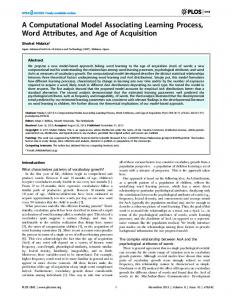
We assume that the collective states of the mass quanta within an elementary particle generate the particle itself, and can be thought of as collectively “coding” for the particular particle that is generated. For example, assuming me is the mass of an electron, we would view an electron as being generated by 2 N = mEe0c mass quanta, in some particular set of collective states, that together code for the properties of an electron. As a result, we represent the mass quanta within an elementary particle as a complete graph, where each mass quantum is represented as a vertex, with each mass quantum vertex connected to all other mass quanta vertices. Note that we are not suggesting that the quanta are necessarily “bonded” together in some fashion, but rather, we use discrete graphs because they are a convenient representational schema for the concepts we will make use of throughout the remainder of this paper. Further, we assume that the state of each quantum of kinetic energy within an elementary particle is fixed, and codes for a particular amount of displacement in a particular direction of motion, that, in the absence of an interaction with some other force or particle, never changes. As a result, we assume that direction of motion is quantized. Since direction of motion appears to be continuous, K must be extremely 18

large.25 Finally, we assume that each kinetic quantum can cause only one mass quantum to change position upon any given click, and thus, we represent each kinetic quantum as an “additional” vertex that is adjacent to exactly one mass quantum vertex. Thus, we assume that the mass quanta within an elementary particle can change positions independently of each other. However, we show in Section 3.3 below that the relative positions of the mass quanta within an elementary particle are approximately constant over time. vm vk

Figure 2: A network of quanta with four clusters. We call each connected graph of quanta a network, and the set of all kinetic quanta adjacent to a given mass quantum, together with that mass quantum, a cluster. In Figure 2, vk is a kinetic quantum, and vm is a mass quantum. Together, vk and vm constitute a cluster. Thus, each network represents a single elementary particle,26 and each cluster within a network will contain exactly one mass quantum vertex, and any number (including zero) of kinetic quanta vertices. The particular particle that is generated by the network will be determined by the collective states of the mass quanta within the network, and the kinetic energy of the resultant particle will be determined by the number of kinetic quanta within the network. Further, we assume that upon each click, exactly one quantum of energy within each cluster will become active, which means that either the active quantum will change states, or its cluster will change position, depending upon whether the active quantum is in a mass state or a kinetic state, respectively. Assumption 3.1. Upon each click, exactly one quantum of energy contained within each cluster will become active, and the probability that a given quantum of energy within a cluster will become active is equal for all quanta within the cluster. Thus, upon each click, we assume that exactly one quantum of energy within each cluster will become active, and the action coded for by the active quantum 25 This also implies an absolute frame of reference from which we can determine direction of motion, which we will address in Section 4 below. 26 We are not suggesting the existence of particles outside of the Standard Model of physics, but there is nothing within this paper that would prohibit the existence of such particles.

19

will determine the next state of the cluster. As such, we can think of R as being applied to the particle upon each click, generating the next state of each cluster within the particle, which will cause a given cluster to either change position, or cause the mass quantum within the cluster to change states. Stated informally, each mass quantum within an elementary particle can be thought of as having a single “vote” on what actions take place within the particle upon each click, but these actions generally a↵ect each cluster individually, and do not impact the particle as a whole. However, in Section 3.2 below, we discuss elementary particle decay, which we assume to be the result of mass quanta changing states over time, and thereby, eventually coding for another particle, or set of particles. Because there is only one quantum of mass energy within each cluster, the greater the kinetic energy within a cluster, the less likely it is that the mass quantum within the cluster will become active upon any given click. Assumption 3.2. If the mass quantum contained within a cluster becomes active upon a given click, then that mass quantum will change from its current mass state to its next mass state, and no other quanta within the cluster will change state or position. Note that Assumption 3.2 assumes that the mass energy within an elementary particle will spontaneously change states. Thus, even in the absence of an interaction with another particle, a quantum of energy that is in a mass state will transition through mass states over time, but will not transition to a kinetic state. Assumption 3.3. If a quantum of kinetic energy becomes active upon a given click, then the entire cluster of which the quantum is a part will change position, traveling the distance coded for by the active quantum, in the direction coded for by the active quantum, and no other quanta of energy within the cluster will change states. Thus, an active quantum of kinetic energy will cause its entire cluster to travel the distance coded for by the quantum, in the direction coded for by the quantum, but will not cause any quanta within the cluster to change states. We define the position of a cluster as the position of its mass quantum, and assume that the relative positions of all quanta within a cluster are constant over time. Since mass quanta always remain in a mass state, and kinetic quanta never change states, in the absence of an interaction with another particle, both the mass energy and kinetic energy of an elementary particle will remain constant. Assumption 3.4. Given an elementary particle with a kinetic energy of EK and mass energy of EM , the time-average of the number of kinetic quanta attached to each cluster within the particle is equal for all clusters, and is given by, qµ =

EK E0 EM E0

20

=

EK . EM

(11)

Thus, we assume that the kinetic quanta within an elementary particle will move from one cluster to another over time, and that as a result, the timeaverage of the kinetic energy of each cluster within the particle will be equal, and given by qµ E0 . In short, we assume that the kinetic quanta within an elementary particle are equally distributed among its mass quanta over time. Note that the distribution of kinetic quanta among the clusters over time has no e↵ect on the total energy of the particle, which remains constant.

3.2

Elementary Particle Decay

In Section 3.1 above, we noted that since the probability that any quantum within a given cluster becomes active is equal for all quanta within the cluster, it follows that the greater the kinetic energy within a cluster, the lower the probability that the single mass quantum within the cluster will become active and thereby change states. Specifically, Assumption 3.4 implies that the expected probability that the mass quantum within a given cluster will become active and thereby change states upon any given click is p = qµ1+1 = EEM . We T can find the probability that k mass quanta will become active upon a given click by assuming that the clusters become active independently of each other, which results in a binomial distribution where the number of trials equals the number of clusters, which is also the number of mass quanta, and each active mass quantum is treated as a “success” event. Assumption 3.5. The probability that k mass quanta change states upon any given click within an elementary particle with a total of NM mass quanta is given by, ✓ ◆ NM k pk = p (1 p)NM k . (12) k Thus, the expected number of active mass quanta upon any given click is pNM . If we assume that the particle is stationary, then p = 1, and as such, every quantum of mass energy within the particle will change states upon each click. Assume that the expected lifetime of the particle is tµ seconds when the particle is stationary. We can express this expected lifetime as a number of t clicks given by kµ = tµ0 . Since the particle is stationary, upon each click, every mass quantum within the particle will change states, and thus, the total number of state changes after kµ clicks is simply kµ NM . We view the particle’s decay as the result of the mass quanta within the particle changing states over time, thereby eventually coding for a di↵erent particle, or set of particles. As such, we view kµ NM as the expected total number of state changes that will cause the particle to spontaneously decay. We view the conservation of total energy during this process as the result of the nature of energy itself, which we view as a physical substance that cannot be created or destroyed, but instead, changes states over time. In contrast, we view the conservation of other properties, such as mass and charge, as the result of the physical transitions codified by R. That is, given the present state of some set 21

of quanta of energy, only certain future states are accessible from that present state, namely those that can be generated by successive application of R to the present state. Thus, given any elementary particle, the set of particles that it can decay into will be a function of the total energy of the particle, and R. Similarly, the expected lifetime of the particle will also be a function of R. For example, if the next state of each mass quantum within an elementary particle is always the current state, then the particle will be perfectly stable. Similarly, if the mass quanta are stuck in a “loop” of states that all code for the same particle, then the particle will be perfectly stable in that case as well. s1 s2

s3 s4 Figure 3: Sequences of collective states. As a general matter, we can create any expected lifetime by simply assuming that at some point, the collective states of the mass quanta within the particle will eventually code for another particle, and adjust the length of that sequence to the desired lifetime of the particle. More realistically, if we allow for n possible sequences of collective states, each of which leads to a collective state that codes for another particle, or set of particles, then the expected lifetime of the particle is the expected value of the amount of time until decay across all such sequences of collective states. For example, in Figure 3, each non-terminal node represents a collective set of states that all code for the same particle, and each terminal node represents a collective set of states that causes the particle to decay into some other particle, or set of particles. As such, the number of clicks until decay along each sequence of states terminating at s2 is 3 clicks. Assuming the branching probability is 12 at each node, the total probability of arriving at any si is 14 ,27 and thus, the expected lifetime of the particle is 52 clicks. As a general matter, if ki is the number of clicks until decay along sequence i, and pi is thePprobability of sequence i, then the expected lifetime of the particle is n tµ = t0 i=1 pi ki . Now assume that a particle with an expected lifetime of tµ seconds when stationary has some velocity, and thus, some kinetic energy. In that case, p < 1, 27 Note that there are two sequences of collective states that terminate at each of s and s , 2 3 each of which has a probability of 18 .

22

and as such, the total expected number of state changes after k clicks is kpNM < kNM . Thus, the number of clicks required to achieve any given expected number of state changes will increase as a function of the kinetic energy of the particle. Specifically, the number of clicks required to achieve an expected number of state changes equal to kµ NM will increase. Assuming kpNM = kµ NM , it follows that T , which is the number of clicks required to achieve an expected number k = kµ EEM of state changes equal to kµ NM . Since kµ NM is the expected number of state changes that will cause the particle to spontaneously decay, it follows that k is in this case the number of clicks that we expect the particle to survive. Let T = EEM . Multiplying by t0 , we can find the expected lifetime of the particle generally, which is given by, t = tµ . If we assume that

=

q 1 1

v2 c2

(13)

, then equation (13) is consistent in form with

the special theory of relativity. However, the reason for this result is due to the presence of kinetic energy within the particle. Further, tµ is a measure of objective time, which we will discuss in greater detail in Sections 3.4 and 4.1 below. Thus, over time, the particle will mature through its states at an objectively slower rate, simply because it is less likely that its mass quanta will become active upon any given click, resulting in a longer expected lifetime.28

3.3

Kinetic Energy and Velocity

Because each quantum of kinetic energy within an elementary particle causes the cluster of which it is a part to travel a particular distance in a particular direction when active, we can think of each kinetic quantum within an elementary particle as a velocity vector vi , such that kvi k, which denotes the norm of the vector, gives the distance traveled by the cluster when that quantum is active. However, we do not assume that all kinetic quanta within a particle code for the same amount of displacement or direction of motion. Thus, both the displacement per click and direction of motion of a cluster can change upon any given click. If p0 is the initial position of a cluster, and the cluster changes position m times, then we can express the final position of the cluster as, pf = p 0 + v i 1 + . . . + v i m . That is, because each kinetic quantum corresponds to a velocity vector, to find the final position of the cluster, we can simply add the velocity vectors that correspond to the kinetic quanta that were active over the interval of time under consideration to the initial position of the cluster. Note that the expected K probability that a cluster will change position upon a given click is 1 p = E ET . 28 Due to the complexity of composite particles, we do not present an analogous model that is specific to the spontaneous decay of composite particles. However, we do present a general model of time-dilation in Section 3.4 below, which would apply to all systems, including composite particles.

23

As such, we can view m as an expectation value, where if k is the number of EK K clicks that have elapsed, then m = (1 p)k = E ET k. Let NK = E0 be the PNK number of kinetic quanta within an elementary particle, and let vT = i=1 vi , which is the sum over all of the velocity vectors corresponding to the kinetic quanta within the entire particle. Assumption 3.6. For any given cluster within an elementary particle, the frequency of each vi in the sum p0 +vi1 +. . .+vim approaches N1K as k increases. That is, because we assume that kinetic quanta move from one cluster to another over time, we assume that, as a result, the frequency of each vi in the sum p0 + vi1 + . . . + vim approaches N1K as k increases, and thus, the number of instances of each vi approaches NmK .29 Therefore, over any interval of time, for each cluster, pf ⇡ p0 + NmK vT . Further, let p0i and p0j , and pfi and pfj , be the initial and final positions of two clusters, respectively. It follows that, kpfi pfj k ⇡ kp0i p0j k, and thus, the relative positions of the clusters are approximately constant over time. In short, we assume that all of the kinetic quanta within an elementary particle circulate among the clusters, causing the overall motion of the individual clusters to be nearly identical over time. Because each quantum of kinetic energy can code for di↵erent directions of motion, the actual total displacement of a given cluster could exceed the straight line distance between its initial and final positions. However, we assume that the displacement per click, and the distances between the clusters, are both so small, that the overall motion is perceived as a single particle traversing a straight line. Specifically, we assume that the observed displacement of a particle after k clicks is NmK kvT k, and thus, the observed velocity of the particle is given by, v=

m NK kvT k

kt0

=

kvT kE0 . ET t0

(14)

Tk Let µ = kv NK , which can be thought of as the e↵ective displacement per kinetic quanta.30 As such, we can express equation (14) as,

v=

EK µ . E T t0

(15)

29 For example, if all of the kinetic quanta within an elementary particle circulate among the mass quanta within the particle as a single group, in a “loop” around the mass quanta, then each kinetic quantum will be attached to each mass quantum exactly once over each pass around the loop. That is, the kinetic quanta repeatedly traverse a Hamiltonian circuit around the complete graph formed by the mass quanta. In that case, each kinetic quantum will be equally likely to become active within any given cluster, and thus, the frequency with which each kinetic quantum is active within a given cluster will be equal for all kinetic quanta over time, and equal within all clusters over time. Because t0 is presumably extremely small, we assume that this frequency is almost exactly N1 for all intervals of time. K 30 Note that if E K = 0, then µ is undefined. However, in that case, the particle is by definition stationary, and thus, we assume that µ is 0.

24

Note that none of the analysis above places anyq restrictions on the value of EK µ µ, and thus, we can always assume that ET t0 = c 1 ( EEM )2 , which implies T r 2 2 ET EM that µ = ct0 .31 In that sense, equation (15) is consistent with the E2 K

special theory of relativity. However, because our analysis places no restrictions on the value of µ, equation (15) does not imply a maximum velocity, which is not consistent with the special theory of relativity. Specifically, equation (15) does not imply that velocity is always bounded by c. This would allow, for example, a particle with mass to travel at a velocity of c, which is consistent with experimental evidence that suggests that neutrinos have a non-zero mass [7], and a velocity of c [1]. Thus, while we assume that = q 1 v2 throughout 1

c2

this paper in order to demonstrate consistency between our model and the special theory of relativity, equation (15), and the neutrino itself, suggest the T possibility that there is a more general formulation of the value given by = EEM that does not restrict the velocity of a particle to a value that is bounded by c. Further, note that for any given µ, Equation (15) is maximized if ET = EK . That is, equation (15) is maximized when the particle consists solely of kinetic quanta. Further, if a given particle consists solely of kinetic quanta, and all such quanta are identical, then each quantum will code for the same amount of displacement in the same direction. As such, in that case, kvT k = NK kvi k, and thus, µ = kvi k will be constant, regardless of the total energy of the particle. Thus, if a particle consists solely of identical kinetic quanta, then the particle will have a constant velocity of tµ0 , regardless of its total energy. As such, we assume that every quantum of energy within a photon is in a kinetic state, and that for any given photon, all quanta within the photon are identical. Further, we assume that all quanta within all photons code for the same amount of displacement. However, unlike elementary particles with mass, we do not make any additional assumptions about the structure of a photon.32 Note that because we assume that a photon is comprised of identical K kinetic quanta, it follows that E ET = 1, and that µ is constant regardless of the photon’s energy. Further, because all quanta within all photons code for a single displacement, the value of µ is uniform for all photons. As such, all photons will have a velocity of tµ0 , which we assume to be c, and a mass of 0, regardless of whether the source that ejected the photon is moving or stationary, and regardless of the energy of the photon. Finally, note that because we allow for di↵erent kinetic quanta to code for di↵erent displacements per click, two particles could have the same kinetic energy and mass energy, yet have di↵erent values for µ, and therefore, di↵erent velocities, even if all kinetic quanta within both particles code for the same direction of motion. Thus, equation (15) implies that we cannot determine the kinetic energy of a particle by measuring its mass and velocity alone, without 31 That said, because we have not proposed a value for t , we cannot, as a practical mat0 ter solve for µ. Nonetheless, the point remains, that as a theoretical matter, there are no restrictions on the value of µ that would prevent us from solving for its value. 32 We will discuss the properties of light in greater detail in Sections 3.5 and 4.2 below.

25

making additional assumptions about the value of µ. Similarly, we cannot determine the velocity of a particle based upon its kinetic energy and mass energy alone. As such, equation (15) would allow for particles that, like the photon, have constant velocities regardless of their energy.

3.4

Moving Clocks and Absolute Time

Consider a stationary clock. Even though the clock is stationary, because it is a clock, it will have some internal machinations that allow it to keep time, and thus, some small amount of kinetic energy. When the clock is stationary, all of the energy contained within the clock codes for the clock itself, which we call “clock quanta”. That is, the mass energy of the clock generates the substance of the clock, and the small amount of kinetic energy within the clock generates the machinations of the clock that cause it to keep time. However, if the clock has some overall velocity, then the kinetic energy associated with that velocity will code for the overall velocity of the clock, and not its mass or its internal machinations. In order to analyze the energy of a moving clock, we will first need to expand Assumption 3.4, which is limited to elementary particles, to all closed systems generally. Assumption 3.7. Given a closed system with a total mass energy of EM , the time-average of the number of kinetic quanta that code for the overall velocity of the system that are attached to each cluster within the system is equal for all EK clusters, and is given by Qµ = E , where EK is the total kinetic energy of the M system that codes for its overall velocity. Assumption 3.7 is a generalization of Assumption 3.4, and implies that, over time, the kinetic quanta that code for the overall velocity of a system are evenly distributed among the mass quanta within the system. As such, Assumption 3.7 would not apply, for example, to the kinetic energy that codes for the internal machinations of a stationary clock, since that energy does not code for some overall velocity, and therefore, would not be evenly distributed among the mass of the clock, but would instead, generally be concentrated in the parts of the clock that cause it to keep time. In contrast, Assumption 3.7 would apply to the kinetic energy that codes for the overall velocity of a moving clock. Further, the amount of time required to achieve this uniform distribution will of course depend upon the system. For example, the distribution of kinetic energy that codes for the overall velocity of a solid object should generally be uniform among the mass of the object, since the rate of collisions between the particles within the object is likely going to be high, causing any uneven distributions of that kinetic energy to be transitory. In contrast, a gas trapped in a volume that is accelerated in a particular direction could require a significant amount of time before the kinetic energy that codes for the resultant overall velocity of the volume is evenly distributed among the particles within the gas. Note that Assumption 3.7 does not imply that the total kinetic energy of each particle within the gas will be equal, or that the motions of the particles within the gas will be identical, but rather, that the average number of kinetic quanta 26

that code for the overall velocity of the volume attached to a given cluster will eventually be equal for all clusters within the volume. Thus, the particles within the gas will still have idiosyncratic motions, just like a moving clock will still have internal machinations, but Assumption 3.7 implies that the particles within the gas will eventually all share in the kinetic energy that codes for the overall velocity of the volume as a whole, in an amount that is, on average over time, in proportion to their respective masses. In the case of a moving clock, we want to know, upon any given click, how many active quanta actually code for the clock itself, as opposed to its overall velocity. Thus, we are not interested in the expected number of active mass quanta per click, but rather, the expected number of active clock quanta per click. We can calculate this by first calculating the probability that any given clock quantum is active within a given cluster, and from that probability, calculate the probability that any given number of clock quanta are active within the entire clock, and finally, find the expected value of that distribution. As such, we view any active clock quantum within a cluster as a “success” event for purposes of our probability distribution. Note that the number of trials is equal to the number of clusters NM = EEM0 within the system, just as it is in the case of an elementary particle. Further, we assume that the clusters are independent of each other, in that the particular quantum that is active within a given cluster is not in any way a function of which quanta are active in any other clusters, and thus, the resultant distribution is again a binomial distribution. Because the clock has some overall velocity, the expected energy of each cluster within the clock will consist of one quantum of mass energy, some very small fractional number of kinetic quanta that code for the machinations of the clock, which we denote by e, and the cluster’s share of kinetic quanta that code for the overall velocity of the clock, which we denote by Qµ . Since an active mass quantum or an active kinetic clock quantum within a cluster would constitute a 1+e success event, the exact expected probability of success is 1+e+Q . The expected µ value of e is the number of kinetic clock quanta divided by the number of mass quanta, which is also the ratio of the kinetic energy divided by the mass energy 1+e C of the clock when stationary. It follows that 1+e+Q = EME+E , where EC is µ T the kinetic energy of the clock when stationary. However, we assume that EC is so small when compared to EM , that the actual distribution is approximated by a distribution with a probability of success given by p = EEM , and that as T a result, the expected number of active clock quanta per click is approximately pNM .33 When the clock is stationary, upon each click, all active quanta are clock quanta, and thus, the total number of active clock quanta after k clicks is simply kNM . We assume that for sufficiently large k, for every kNM of active clock 33 Disregarding the value of E would be reasonable for any system with internal machinaC tions that have a kinetic energy that is several orders of magnitude smaller than the system’s mass energy, which is likely to be the case for any reasonable construction of a clock. For EC example, even in the case of a clock driven by a pendulum, the value of E will likely be

proportional to

v2 , c2

M

where v is the velocity of the pendulum.

27

quanta, there is a single value ⌧ such that the time reported by the clock is incremented by approximately kNM ⌧ . That is, each active clock quantum can be thought of as causing the time reported by the clock to increase by ⌧ .34 If the clock is accurate, then when it’s stationary, after k clicks, the time reported by the clock should increase by kt0 . Thus, kt0 = kNM ⌧ , which implies that NM ⌧ = t0 . When the clock is moving, the expected number of active clock quanta after k clicks is kpNM . Therefore, the expected total change in time reported by the clock after k clicks is t = k EEM NM ⌧ = kt0 . T We assume that t¯ = kt0 is measured by a zero energy clock, which we define as a clock that consists of only clock quanta, and thus, no kinetic energy beyond that which is necessary to allow the clock to keep time.35 As a theoretical matter, a single mass quantum in isolation would constitute a zero energy clock, since its state would change once per click. Thus, we assume that all active quanta become active simultaneously everywhere, and therefore, we treat the number of clicks that have elapsed as an objective measure of time. It follows that, t=

t¯

.

(16)

Note that equation (16) calculates time-dilation relative to t¯, which we assume to be a measure of absolute time, as measured by a zero energy clock, and thus, while equivalent in form, equation (16) is not entirely consistent with the special theory of relativity. Further, note that equation (16) is the mechanical result of the presence of additional kinetic energy that codes for the overall velocity of the clock.36 Moreover, while we have framed this discussion in terms of a moving clock, the same reasoning applies to any system with some overall velocity. That is, a system with some overall velocity will take more objective time to progress through the internal changes that would have occurred in an identical stationary system. Thus, all moving systems will undergo time-dilation in accordance with equation (16) due to the presence of kinetic energy within the system that codes for the overall motion of the system. For example, the biological processes of a living organism with some overall velocity would therefore progress slower, since the quanta that code for its biological processes will be active less often due to the presence of the kinetic quanta that code for its 34 As

a practical matter, each clock quantum will not contribute equally to the clock’s time keeping processes. For example, the mass quanta of an ordinary clock presumably code for stable matter, and thus, their changing states presumably do not contribute to the clock’s time keeping processes. Thus, we are tacitly assuming that after a sufficiently large number of k clicks have elapsed, the average increment in time per active clock quantum always converges 2 +···+ k to a single value ⌧ ⇡ 1 + kN , where i is the increment in time reported by the M clock upon the i-th click. Because t0 is presumably extremely small, we assume that the total change in time reported by the clock can always be expressed as kNM ⌧ = 1 + 2 + · · · + k . 35 We will revisit this topic in greater detail in the context of inertial frames in Section 4.1 below. 36 We present no theory of gravity, and thus, no theory of time-dilation due to gravity. As such, all references to time-dilation in this paper are references to time-dilation due to the velocity of a system alone.

28

overall velocity. Finally, note that it is ultimately the number of kinetic quanta that code for the overall velocity of a system that causes the system to experience timedilation, not its velocity, which is a consequence of that kinetic energy in the first instance. For example, even if two particles have the same mass energy and kinetic energy, the particles can nonetheless have di↵erent velocities if they have di↵erent values for µ. However, because both particles have the same T mass energy and kinetic energy, the value given by = EEM is the same for both particles. Thus, both particles will experience the same amount of timedilation, despite traveling at di↵erent velocities. Therefore, as a general matter, we cannot determine based upon the velocity of a system alone, without making additional assumptions about the value of µ.

3.5

The Doppler E↵ect

Because we do not need to assume that the measured velocity of light is constant in all inertial frames in order to achieve time-dilation, we do not make that assumption.37 As a result, the classical Doppler equations, which distinguish between the motions of a light source and a detector, would apply to our model, as adjusted to account for time-dilation, which we discuss in the paragraphs below. But rather than present the classical explanation for the Doppler e↵ect, which is in no way inconsistent with our model, since we can always assume that quanta generate a wave, we present an explanation that is unique to our model of energy. Specifically, because we view photons as consisting solely of kinetic quanta, we can view a light source as ejecting kinetic quanta. As such, over any interval of time, we can consider the P average distance between quanta ejected by a N stationary light source µs = N1 i=1 li , where each li is the distance between a given quantum and the quantum that is closest to it in the direction the light is traveling, and N is the number of such pairs of quanta traveling between the source and the detector at a given moment in time. We assume that µs is approximately constant over time. Thus, at any point along the detector in Figure 4, the expected time between quanta is ts = µcs . As such, when the source and the detector are both stationary, we can express the expected amount of energy incident upon any single point along the detector over an interval of time t as Es = E0 tts . As the velocity of the source changes, the average distance between each such pair of quanta will also change, just as the distance between each wave crest will change when we view the light source as generating a wave.38 Thus, the amount of energy per unit of time that is incident upon a given point along the detector will vary with the velocity of the source, increasing when the source moves towards the detector, and decreasing when the source moves away from the 37 We present an analysis of the velocity of light as measured within a moving inertial frame in Section 4.2 below. 38 For the moment, we will ignore any red-shift due to time-dilation, which we will address in the paragraphs below.

29

lj Detector Source

li

Figure 4: A light source ejecting quanta towards a detector. detector. Specifically, if the distance between two quanta is li when the source is stationary, then when the source has a velocity of v towards the detector, the expected distance between the two quanta will be P li vts . Thus, the average N distance between any two quanta will be µv = N1 i=1 (li vts ) = µs vts . As such, the expected time between quanta at any point along the detector is tv = µs cvts . Thus, the amount of energy incident upon any point along the detector over an interval of t seconds is Ev = E0 ttv = Es c c v . Note that if the source is moving away from the detector, then the same analysis would apply, but v would in that case be negative. Further, if the source is moving at an angle of ✓ relative to the direction of its light, then v = cos(✓)v 0 , where v 0 is the velocity of the source.39 Thus, as a source moves in the direction of its light, the ejected quanta become more concentrated, whereas when a source moves away from the direction of its light, the ejected quanta become more di↵use. If we assume that Ev and Es are partitioned among an equal number of M photons, then Ev = M hfv , and Es = M hfs , for some frequencies fv and fs . Under this view, the frequency of the light incident upon the detector is determined by the rate at which energy is incident upon a single point along the detector. In contrast, we view the luminosity of the light as determined by the rate at which energy is incident upon the entire surface of the detector.40 Since Ev = Es c c v , it follows that, fv = fs

c

. (17) c v Now consider the case of a stationary source, and a detector moving toward that source. Since we do not assume that the velocity of light is constant in every inertial frame, it follows that an analogous e↵ect would occur when the detector moves towards or away from a stationary source, causing the number of quanta incident at any point along the detector per unit of time to increase as the detector moves towards the source, and decrease as the detector moves away from the source. However, the actual average distance between quanta is unchanged, since the source is stationary. Instead, the average amount of time 39 That is, a given quantum is always “paired” with another quantum that lies on the same line connecting the source to the detector for purposes of calculating each li . As such, if the source is moving perpendicular to the direction of its light, that motion will not impact the average distance between the quanta. 40 Thus, a more luminous source will leave fewer “dark spots” on the surface of the detector.

30

between quanta at any point along the detector will vary with the velocity of the detector. Specifically, the expected time between quanta when the detector µs is moving towards a stationary source is tv = c+v . In this case, it follows that, c+v . (18) c Note that if the detector is moving away from the source, then the same analysis would apply, but v would in that case be negative. Further, if the detector is moving at an angle of ✓ relative to the direction of the light, then v = cos(✓)v 0 , where v 0 is the velocity of the detector. Moreover, note that in all cases, we simply change the time at which the quanta from the source arrive at the detector, and thus, total energy is conserved. That is, the quanta ejected by a moving source will be more concentrated than that of a stationary source if the source is traveling in the direction of its light, and more di↵use if the source is traveling away from the direction of its light. Similarly, a detector that is moving towards a stationary source will experience a more concentrated field of quanta, whereas a detector that is moving away from a stationary source will experience a more di↵use field of quanta, though in this case the actual distance between quanta is unchanged. Thus, in all cases, total energy is conserved, since the number of quanta ejected by the source over any interval of time is not a↵ected by the motion of the source or the detector, except for the e↵ects of time-dilation, which we now address in the paragraphs below. We can account for the red-shift associated with time-dilation, while still conserving total energy, by assuming that the rate at which energy is ejected or absorbed by a system is a↵ected by time-dilation in the same way that all internal processes of a moving system are a↵ected by time-dilation. Specifically, assume that a stationary source ejects quanta at a rate of Es = t¯N E0 Joules every t¯ seconds of absolute time, for some N . We assume that when the source ¯ has some overall velocity, it will eject quanta at a rate of Ev = t N E0 = 1 Es every t¯ seconds. That is, it will take longer for the source to eject the same amount of energy because all internal processes occur at a slower rate as a consequence of time-dilation, including the ejection of energy. If we assume that this energy is again in the form of M photons, then M hfv = 1 M hfs , where fs is the frequency of the source when stationary. Thus, fv = 1 fs , causing a red-shift. We assume that the same arguments in the paragraph above apply to a moving detector. Specifically, while the energy incident upon the surface of the detector is of course not a↵ected by time-dilation’s e↵ects on the detector, we assume that the rate at which energy is exchanged by the atoms within the detector is a↵ected by time-dilation, in the same way that the atoms within a source of light eject energy at a slower rate due to time-dilation. That is, we assume that time-dilation causes the atoms within the detector to exchange the energy of the photons incident upon the detector at a lower rate of energy per unit of time, just like a moving source will eject less energy per unit of time due to time-dilation. Thus, the atoms within a moving detector will exchange less fv = fs

31

energy per unit of time, ultimately resulting in a lower detected frequency of 1 fs . If we assume that = q 1 v2 , then combining the Doppler e↵ect with the 1

c2

red-shift due to time-dilation yields the following equation for the frequency of light measured by a stationary detector: r c v2 f = fs 1 . (19) c v c2 In the case of a stationary source, we have the following: r c+v v2 f = fs 1 . (20) c c2

Note that equation (19) is consistent in form with the special theory of relativity. However, equation (20) is not, since we have distinguished between the motions of the detector and the source. Applying the special theory of relativity, we would not distinguish between the motion of the detector and the motion of the source, but would instead only calculate their relative velocity. As such, we would treat the case of a detector moving towards a stationary source with a velocity of v in the same manner that we would treat the case of a source moving towards a stationary detector with a velocity of v. Thus, we can compare the energy per photon as predicted in that case by our model, with that predicted by the special theory of relativity, by taking the di↵erence between equations (19) and (20), and multiplying by Planck’s constant h: ✓ ◆ 1 c c+v = hfs . c v c As such, will be very small for even substantial values of v and fs . In order to test the validity of equation (20), a detector could simply be accelerated towards a stationary source, with the resultant detected frequencies measured and compared to the frequencies predicted by equations (19) and (20).41

4 4.1

Inertial Frames and the Velocity of Light Inertial Frames

We assume that a single quantum of mass energy would not just appear to be stationary, but rather, would in fact be stationary because it has no kinetic energy with which it can move. As such, we can define a truly stationary coordinate system by reference to a set of orthogonal vectors whose distances from a single mass quantum are fixed. We call any such coordinate system an absolute coordinate system. The absolute distance between any two 41 Note that experiments such as [13] involving a rotating M¨ ossbauer detector would not constitute tests of the validity of equation (20), since the detector is not moving towards the source in these experiments, but is instead rotating around the source.

32

points, measured in meters, can then be determined by reference to any absolute coordinate system, and thus, we assume that the absolute distance between any two points is equal in all absolute coordinate systems. We define the change in absolute time as the number of clicks that have elapsed multiplied by t0 , which we assume to be equal to the change in time reported by any zero energy clock over that same number of clicks. We define absolute displacement as the absolute distance between the initial and final positions of a system over some interval of absolute time. We define absolute velocity as the ratio of the absolute displacement of a system over a given interval of absolute time divided by the length of the interval of time. We define a zero energy inertial frame as any set of systems whose positions are constant in an absolute coordinate system. In general, we define an inertial frame as any set of systems whose absolute distances from each other are constant. We define the velocity of an inertial frame as the absolute velocity of any system within the inertial frame, which will be equal for all such systems. Thus, we can define a coordinate system by reference to a set of orthogonal vectors whose absolute distances from any system within a given inertial frame are constant. We call any such coordinate system an inertial coordinate system. We assume that the distance between any two points in a given inertial coordinate system is equal to the absolute distance between those two points. Thus, we reject the notion of length contraction implied by the special theory of relativity. However, we do not assume that measurements of displacement are constant in all inertial frames. Rather, in general, we define displacement as the distance, measured in meters, between the initial and final positions of a system in some inertial coordinate system over some interval of time, which we define as the change in time reported by a clock within the applicable inertial frame. Finally, we define velocity as the ratio of the displacement of a system over a given interval of time divided by the length of the interval of time. Consider a simple example of a bus traveling with a constant absolute velocity of v meters per second. All seated passengers on the bus are part of the same inertial frame that includes the bus itself, and all other objects that are traveling at the same absolute velocity as the bus, which, therefore, appear stationary relative to the bus. However, if a passenger runs from one end of the bus to the other, that passenger is not part of the inertial frame of the bus for so long as the passenger is running, and is instead an object whose velocity can be measured from within the inertial frame of the bus. Assume that the bus is 12 meters long, that the bus is traveling forwards, and that the passenger runs from the rear of the bus to the front of the bus in 5 seconds of absolute time. Because we assume measurements of distance are uniform in all inertial frames, the length of the bus is uniform in both the inertial frame of the bus and any zero energy inertial frame. However, the displacement of the running passenger is not uniform in all inertial frames. Specifically, the displacement of the running passenger as measured from the inertial frame of the bus is 12 meters. In contrast, the absolute displacement of the running passenger is 5v + 12 meters. Similarly, the amount of time that has elapsed is also not uniform across all 33

inertial frames. Specifically, the absolute change in time is t¯ = 5 seconds, but a clock on the bus will report a change in time of t = 5 seconds. Thus, the absolute velocity of the passenger is 5v+12 meters per second, whereas the velocity 5 of the passenger as measured from within the inertial frame of the bus is 12 5 meters per second. Now assume that the passenger runs from the front of the bus to the back of the bus in 5 seconds. The absolute velocity of the passenger is therefore 5v 5 12 meters per second, whereas the velocity of the passenger as measured in the inertial frame of the bus is again given by 12 5 . We assume that the reason the absolute velocity of the passenger is less than v while running is because the kinetic energy of the passenger decreases. Because we assume that total energy is conserved, we assume that the kinetic energy lost by the passenger is gained by the bus. However, because the bus has a very large mass, the impact of this additional kinetic energy on the velocity of the bus is negligible.

4.2

Measuring the Velocity of Light

In some sense, the measurements made in the inertial frame of the bus are simply incorrect, since they are based upon limited information. That said, historically, it has generally been assumed to be impossible for an observer to determine their absolute velocity. This assumption is not specific to the special theory of relativity, and in fact dates back to at least as early as 1632, when Galileo asserted that all motion is relative [9]. However, because of our model of energy, all motion is by definition absolute, since it is always driven by the prescence of some definite number of kinetic quanta, even though measurements of displacement are not uniform across all inertial frames. Because our model implies a constant, and universal absolute velocity of light, but nonetheless allows for time-dilation and non-uniform measurements of displacement within inertial frames, we argue below that it is possible for an observer to determine their absolute velocity by measuring the velocity of light using a clock within the observer’s inertial frame. Thus, our model implies that the measured velocity of light is not uniform in every inertial frame, though our model implies that the absolute velocity of light is always exactly c. This initially appears contrary to over a century’s worth of experimental evidence demonstrating that the measured velocity of light is always extremely close to the exact value of c [8]. However, even though high precision measurements of the velocity of light on the surface of the Earth show little deviation from the exact value of c, these results simply imply that the measured deviations are small enough to disregard in the absence of a deliberate e↵ort to search for the predictable, minute deviations we discuss below. As discussed above, our model of the photon necessarily implies that the absolute velocity of a photon is constant regardless of the velocity of its source. Thus, a photon will always have an absolute velocity of c, regardless of the velocity of its source. However, we also assume that the direction of motion of a photon is independent of the velocity of its source.

34

Assumption 4.1. If a source ejects photons at an angle of ✓ relative to some absolute coordinate system when stationary, then that source will eject photons at an angle of ✓ relative to that same absolute coordinate system when moving in any direction at any velocity. As such, we assume that a source will always eject photons at the same angles, regardless of the velocity of the source.42 Thus, a photon does not participate in the velocity of its source in any manner whatsoever, but is instead ejected at a constant velocity and in a direction that does not depend upon the direction of the motion of its source. For example, assume that an observer is part of an inertial frame with a velocity of v. Further, assume that the observer has an apparatus that consists of a clock, a light source, a mirror, and a detector located within the source, as set forth in Figure 5. Thus, the apparatus can measure the two-way velocity of light in that inertial frame. Further, assume that the distance from the source to the mirror is L, and thus, the round-trip displacement of a photon through the apparatus as measured within the inertial frame is 2L. As noted above, we assume that the distance between the source and the mirror is uniform in all inertial frames, whereas the displacement of the photon over a round-trip, and the amount of time it takes for the photon to complete a round-trip, are not uniform in all inertial frames.

Mirror

L vy Source / Detector

vz vx

Figure 5: A light source with a detector. Thus, the velocity of light as measured in a given inertial frame is not uniform across all inertial frames. Specifically, assume that the velocity of the inertial frame is v = ||(vx , vy , vz )||, where vx is the velocity of the inertial frame in the direction parallel to the line that connects the surface of the source to the surface of the mirror. It follows that the absolute displacement of the photon as it travels from the source to the mirror is L + t¯1 vx , where t¯1 is the absolute time it takes for the photon to travel from the source to the mirror. That is, Assumption 4.1 implies that the velocity of the inertial frame in the y and z directions simply changes the location that the photon is incident upon the mirror and the detector, and does not alter the absolute displacement of the photon. Since the absolute velocity of light is c, it follows that the absolute displacement of the photon is also given by ct¯1 = L + t¯1 vx , and thus t¯1 = c Lvx . Similarly, the absolute displacement of the photon over the return path from 42 We are assuming that the orientation of the source does not change as a result of its velocity.

35

L the mirror back to the source is L vx t¯2 , and thus, t¯2 = c+v . Thus, the total x absolute time and absolute displacement over a round-trip are, respectively, given by,

t¯ = L(

1 c

vx

+

1 ), c + vx

(21)

and, d¯ = 2L + Lvx (

1 c

vx

1 ). c + vx

(22)

As such, the absolute velocity over the round-trip is simply c. In contrast, the round-trip displacement as measured within the inertial frame is 2L, and ¯ the total change in time as measured within the inertial frame is t = t . Note that is a function of the kinetic energy of the apparatus, which, as discussed in Section 3.4 above, cannot be determined by reference to the absolute velocity of the apparatus alone, without making additional assumptions about the value of µ. In contrast, the absolute displacement d¯ is a function of only the absolute velocity of the apparatus in the x direction. Thus, the velocity of light, as measured within in the inertial frame using the apparatus set forth in Figure 5, is given by, vx2 ). (23) c Now assume that we rotate the apparatus. It follows that vx , which is a measure of absolute velocity, will increase or decrease, and thus, our model implies that the velocity of light is not necessarily independent of the direction in which it is measured. However, note that equation (23) is specific to two-way measurements of the velocity of light using an apparatus of the type set forth in Figure 5, and thus, our model could imply di↵erent predicted variations from the exact value of c using other methods of measuring the velocity of light.43 Experiments have shown that it is possible for a moving clock to run slower than a clock that is stationary relative to the surface of the Earth (see [11]), and thus, the absolute velocity of the Earth cannot be 0.44 However, it could be the case that the absolute velocity of the Earth is substantially less than its orbital velocity around the Sun. For example, if we assume that we can reliably measure displacements of one nanometer (10 9 m),45 and we assume that L = 1 meter, then in order for the di↵erence in displacement given by d¯ 2L to be ignored or undetected, it follows that vx must be less than approximately 6703.56 meters per second. While substantially less than the orbital velocity of cv = (c

43 See

[8] for examples of other methods of measuring the velocity of light. that were the case, then any clock on the surface of the Earth would constitute a zero energy clock 45 For example, an interferometer could be used to measure displacements on this scale. However, there could be other methods that are even better suited for measuring minute deviations from the exact value of c (see [8] generally). We have chosen an apparatus of the type in Figure 5 for purposes of illustration because of its simplicity. 44 If

36

the Earth, which is roughly 30, 000 meters per second, it is approximately 14.57 times greater than the rotational velocity of the Earth, which is approximately 460 meters per second. Now assume that we repeatedly rotate the apparatus, measuring the value of cv in each such orientation. Because the kinetic energy of the apparatus will not depend upon its orientation, it follows that will be constant in any given inertial frame, regardless of the orientation of the apparatus. Further, if we find some orientation for which our measurement of cv is minimized, then equation (23) implies that we have in that case pointed the apparatus in a direction that maximizes vx , which must be the actual direction of motion of the inertial frame. If we assume that = q 1 v2 , where v is the absolute velocity of the inertial 1

c2

frame, then in that case vx = v.46 In short, we can rotate the apparatus, and eventually find some orientation which minimizes cv , our measured velocity of light, and because v does not depend upon the orientation of the apparatus, in that case, equation (23) implies that vx = v. Thus, we can in that case solve for the absolute velocity of our inertial frame, which will be, p v¯ = c2 c2v . (24)

Further, recall that time as measured within any inertial frame is given by ¯ t = t . Since we can measure v by maximizing vx , and thereby derive , then for any change in time t measured within an inertial frame, we can solve for the absolute change in time t¯ = t .47

46 As

noted above, we are ignoring any time-dilation due to gravity. results presented in this paper, if true, would clearly have significant consequences for other areas of physics, particularly theories of electrostatic charge and electromagnetism. We concede that a proper treatment of these topics would require a significant undertaking, and thus, we view these topics as beyond the scope of this paper. 47 The

37

References [1] Adamson, P., et al. Measurement of neutrino velocity with the minos detectors and numi neutrino beam. Physical Review 76, 7 (2007). [2] Bennett, C. H. Demons, engines and the second law. Scientific American 257, 5 (1987), 108–116. [3] Bethe, H. A. On the annihilation radiation of positrons. Proceedings of the Royal Society of London, Series A 150, 869 (1935), 129–141. [4] Burke, D. L., et al. Positron production in multiphoton light-by-light scattering. Physical Review Letters 79, 9 (1997), 1626–1629. [5] Colgate, S. A., and Gilbert, F. C. Electron-positron annihlation in flight. Physical Review 89, 4 (1953), 790–792. [6] Compton, A. H. A quantum theory of the scattering of x-rays by light elements. Physical Review 21, 5 (1923), 483 – 502. [7] Drexlin, G., Hannen, V., Mertens, S., and Weinheimer, C. Current direct neutrino mass experiments. Advances in High Energy Physics 2013 (2013). [8] Evenson, K., and Petersen, F. Laser frequency measurements, the speed of light, and the meter. Topics in Applied Physics 2 (1976), 349 – 368. [9] Galilei, G. Dialogue Concerning the Two Chief World Systems. 1632. [10] Grunwald, P., and Vitanyi, P. Shannon information and kolmogorov complexity. eprint arXiv:cs/0410002 (2004). [11] Hafele, J. C., and Keating, R. E. Around-the-world atomic clocks: Observed relativistic time gains. Science 177, 4044 (1972), 168 – 170. [12] Huffman, D. A. A method for the construction of minimum-redundancy codes. Proceedings of the IRE 40, 9 (1952), 1098 – 1101. [13] Kundig, W. Measurement of the transverse doppler e↵ect in an accelerated system. Physical Review 129, 6 (1963), 2371– 2375. [14] Maruyama, K., Nori, F., and Vedral, V. The physics of maxwell’s demon and information. Reviews of Modern Physics 81, 1 (2009), 1–23. [15] Millikan, R. A. A new modification of the cloud method of measuring the elementary electrical charge, and the most probable value of that charge. Physical Review 29, 6 (1909), 560–561. [16] Millikan, R. A. A direct photoelectric determination of planck’s h. Physical Review 7, 3 (1916), 355–388. 38

[17] Shannon, C. E. A mathematical theory of communication. The Bell System Technical Journal 27, 3 (1948), 379–423. [18] Turing, A. M. On computable numbers, with an application to the entscheidungsproblem. Proceedings of the London Mathematical Society s2-42, 1 (1937), 230–265. [19] Turing, A. M. Systems of logic based on ordinals. Proceedings of the London Mathematical Society s2-45, 1 (1939), 161–228. [20] Vanderlooy, S., and Sprinkhuizen-Kuyper, I. G. An overview of algorithmic randomness and its application to reliable instance classification. Technical Report 07-02, Universiteit Maastricht (2007).

39