A computational model that explores the effect of ... - bioRxiv

bioRxiv preprint first posted online Jun. 19, 2017; doi: http://dx.doi.org/10.1101/152066. The copyright holder for this preprint (which was not peer-reviewed) is the author/funder. It is made available under a CC-BY-NC-ND 4.0 International license.

A computational model that explores the effect of environmental geometries on grid cell representations Samyukta Jayakumara, Rukhmani Narayanamurthya, Reshma Ramesha, Karthik Somanb, Vignesh Muralidharanb, and V. Srinivasa Chakravarthyb# a

Dept. of Biotechnology, Rajalakshmi Engineering College, Chennai, Tamil Nadu, India b Bhupat and Jyoti Mehta School of Biosciences, Department of Biotechnology, Indian Institute of Technology Madras, Chennai, Tamilnadu, India-600036.

# - Corresponding Author Address: V. Srinivasa Chakravarthy, 505, Department of Biotechnology Bhupat and Jyoti Mehta School of Biosciences Building Indian Institute of Technology Madras Chennai 600036, India Tel: (+91)-44-2257-4115(O) Fax: (+91)-44-22574102 E-mail: [email protected]

1


Abstract Grid cells are a special class of spatial cells found in the medial entorhinal cortex (MEC) characterized by their strikingly regular hexagonal firing fields. This spatially periodic firing pattern was originally considered to be invariant to the geometric properties of the environment. However, this notion was contested by examining the grid cell periodicity in environments with different polarity (Krupic et al 2015) and in connected environments (Carpenter et al 2015). Aforementioned experimental results demonstrated the dependence of grid cell activity on environmental geometry. Analysis of grid cell periodicity on practically infinite variations of environmental geometry imposes a limitation on the experimental study. Hence we analyze the grid cell periodicity from a computational point of view using a model that was successful in generating a wide range of spatial cells, including grid cells, place cells, head direction cells and border cells. We simulated the model in four types of environmental geometries such as: 1) connected environments, 2) convex shapes, 3) concave shapes and 4) regular polygons with varying number of sides. Simulation results point to a greater function for grid cells than what was believed hitherto. Grid cells in the model code not just for local position but also for more global information like the shape of the environment. The proposed model is interesting not only because it was able to capture the aforementioned experimental results but, more importantly, it was able to make many important predictions on the effect of the environmental geometry on the grid cell periodicity.

2


Introduction Spatial navigation is essential for the survival of a mobile organism. Entorhinal cortex (EC), an important sub-cortical area that forms input to the hippocampus, was reported to have neurons known as grid cells which fire when the animal is at points that have a spatially periodic structure(Hafting, Fyhn et al. 2005). Since the periodicity encountered is often hexagonal, these cells are further known as hexagonal grid cells(Hafting, Fyhn et al. 2005). Albeit grid cells were initially discovered in rats(Hafting, Fyhn et al. 2005), these cells have also been reported in mice(McHugh, Blum et al. 1996; Rotenberg, Mayford et al. 1996; Fyhn, Hafting et al. 2008), bats(Ulanovsky and Moss 2007; Yartsev, Witter et al. 2011), monkeys(Ono, Nakamura et al. 1993; Rolls and O'Mara 1995; Rolls, Robertson et al. 1997; Killian, Jutras et al. 2012) and humans(Ekstrom, Kahana et al. 2003; Jacobs, Weidemann et al. 2013; Moser, Roudi et al. 2014). Experimental studies in human adults who are at genetic risk for Alzheimer’s disease have reported that the neural degeneration originates in the EC, with the loss of grid cell representations causing further impairment of spatial navigation performance of the patient (Kunz, Schröder et al. 2015). Preliminary studies on the effects of environmental geometry on spatial cells such as place cells (Jeffery and Burgess12 2006) and grid cells have been conducted. Place cells are critical for coding the animal’s position in space. They fire when the animal is situated in a particular space of the environment known as its firing field (O'Keefe and Dostrovsky 1971). Remapping of place cells occurred when sufficient changes to the geometry (Lever, Wills et al. 2002), color (Bostock, Muller et al. 1991) or odor (Anderson and Jeffery 2003) of the environment were made. Grid cells are equally crucial for spatial navigation by path integration i.e., tracking position by integrating self-motion even without the presence of external sensory landmarks(Hafting, Fyhn et al. 2005; Fuhs and Touretzky 2006; McNaughton, Battaglia et al. 2006; Burgess, Barry et al. 2007; Hasselmo, Giocomo et al. 2007; Moser, Roudi et al. 2014; Bush, Barry et al. 2015). Grid cells have been proposed to have a role in computing directional vector between the start and goal location (which was termed as vector navigation) that further aids the animal in reaching its goal location(Bush, Barry et al. 2015). The variation of the grid scale across the dorsal to ventral medial entorhinal cortex (MEC) axis(Brun, Solstad et al. 2008; Stensola, Stensola et al. 2012), acts like a ruler with different resolutions to measure the distance 3


traversed by the animal from its starting location. The aforementioned features of the grid cells help the animal to navigate the environment efficiently. MEC conveys spatial information into the hippocampus (Barnes, McNaughton et al. 1990; Quirk, Muller et al. 1992;Fyhn, Molden et al. 2004). It is believed that the dynamic representation of the spatial location of an animal is created and updated by the MEC and the grid cells are a proof of it(Savelli, Yoganarasimha et al. 2008). Hargreaves et al(2005) initially recorded MEC grid cells from an environment (Hargreaves, Rao et al. 2005). Since the size of the environment was relatively small, the neurons did not show obvious grid like firing patterns. It was very ambiguous in prior studies whether all spatially modulated cells in the MEC were variants of the grid cells or whether a subset resembled the place cells of the hippocampus (Savelli, Yoganarasimha et al. 2008). Savelli et al (2008) conducted an experiment where the rats were allowed to forage a small box which was placed inside a larger box. After sometime, the small box was removed from the large box without removing the rats and now the rats foraged the larger box for the rest of the experiment. It was observed that some cells that showed place cell like response in the small box, showed grid cell like response in the larger box and the cells showing boundary cell like response showed no change upon the removal of the small box. The aforementioned experiments gave two inferences: Firstly, it put forth that there were two major classes of spatial neurons, the grid cells and the boundary cells. The boundary cells may therefore be binding the grid cell firing to the boundaries of the environment. Secondly, the experiment strongly demonstrated that the spatial firing of the MEC cells were strongly influenced by the boundaries of the environment, in the sense that representation of the MEC cells changed predominantly when the local cues of the environment were altered. In this paper, we are addressing the second inference from a purely computational point of view. The minimal remapping of the grid fields across the environment made grid cells to be the universal metric for navigation (Hafting, Fyhn et al. 2005). But this feature of grid field invariance across the environment was contested by the experiment conducted by O’Keefe(Krupic, Bauza et al. 2015)wherein rats were allowed to forage inside differently shaped environments such as circle, square, hexagon and trapezoid. Analysis of grid cell activity in each environment revealed that the hexagonal grid field symmetry was affected by the symmetries of the environmental shape. Circle, the most symmetric environment, had a regular hexagonal firing 4


field. As the number of axes of symmetry dropped, the regular hexagonal firing field started to transform into a skewed hexagonal field. This experimental study pointed out that grid cell firing fields were not invariant with respect to the environment but exhibit a definite dependence on the geometry of the environment. Another interesting experimental study(Carpenter, Manson et al. 2015)considered how grid cells responded when the animal foraged inside similar environments connected by a corridor. A key result of the study was that initially the grid fields in each room had a high spatial correlation between them; as the time progressed, this correlation decreased and the grid fields in the two environments became a continuum, forming a global representation of the connected pair of environments. This study revealed a new face of the grid cell coding, whereby the periodic firing fields of the grid cell could rearrange among themselves to reflect the global shape of connectivity of the environment. Most of the experimental studies on grid cells were performed on either square or circular environments, and have not explored the rich possibilities of environmental geometries. Apart from the study of Krupicet al (2015) (Krupic, Bauza et al. 2015),to the best of our knowledge, no experimental studies have been conducted on grid cells under varying environmental geometries. Theoretical studies have been made on grid cell coding in non-Euclidean space(Urdapilleta, Troiani et al. 2015)which came up with the prediction of variation in the hexagonal pattern of firing field to heptagonal pattern with the change from Euclidean to non-Euclidean space. But the problem of studying grid cell coding as a function of practically infinite variations of the environmental geometry poses a Himalayan challenge to spatial cell researchers. Hence, we propose to classify environmental geometries into the following four broad categories and study the emergent grid fields using computational modeling.

i.

Connected environments

ii.

Convex shaped environments

iii.

Concave shaped environments

iv.

Regular polygon environments with varying number of sides

The aforementioned studies, from a pure computational point of view, would result in a better understanding of the spatial encoding inside the brain done by the grid cells. We show that our 5


simulations not only explain and confirm earlier studies, but also make a number of testable predictions verifiable by experiment. Methods

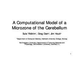
Fig.1: Model architecture. Arrows show the direction of flow of information from one hierarchy to the next.

To achieve the goal of studying the effect of environmental geometry on grid cell coding, we used the model described in(Soman, Muralidharan et al. 2016) with slight modification (Fig.1) as explained below. The model basically has three stages as described below. a. Direction encoding stage This Head Direction (HD) stage forms a neural representation for the direction in which the animal moves. In our earlier model, the direction features were(Soman, Muralidharan et al. 2016) extracted from the limb oscillations of the animal that made the model more biologically plausible. But here we simplified this stage by directly supplying velocity inputs to the model so that additional constraints on the curvature of the trajectory could be circumvented.

6


To obtain a directional map, a Self Organizing Map (SOM) was trained(Kohonen 1982) using two dimensional inputs from a unit circle. The response equation of the SOM neuron is given as: (1)

 HD   TW ψ is the two dimensional input given to the SOM such that ψ = [cos(θ) sin(θ)] where θ is the actual direction of navigation

W is the afferent weight matrix of the SOM, where each weight vectors are normalized. b. Oscillatory Path Integration (PI) stage This stage consists of a two dimensional array of Hopf phase oscillators, which has oneto-one connections with the HD layer. The directional input from eqn. (1) is fed to the phase dynamics of the oscillator so that each component of the positional information is encoded as the phase of each oscillator. The dynamics of phase oscillator is given as

d ( u (i, j ))    v (i, j )[ PI   s HD (i, j )]  u (i, j )[   ( u (i, j ) 2  u (i, j ) 2 )] dt

(2)

d (  v (i, j ))  u (i, j )[ PI   s HD (i, j )]   v (i, j )[   ( u (i, j ) 2   v (i, j ) 2 )] dt

(3)

χ is the state variable of the PI oscillator. β is the spatial scale parameter. s is the speed of the navigation such thats = ||X(t)-X(t-1)|| where X is the position vector of the animal. μis the parameter that controls the limit cycle behavior of the oscillator. Here μ is taken as 1. c. Lateral Anti Hebbian Network (LAHN) stage LAHN is an unsupervised neural network(Földiák and Fdilr 1989) that extracts the high variance features from the input. The network has Hebbian afferent and anti-Hebbian lateral connections. The response of the network is given by the following equation.

7


m

n

j 1

k 1

(4)

i (t )   qij  j (t )   wik k (t  1) qis the afferent weight connections and wis the lateral weight connections. ξis the response of the network.

The afferent connections are updated by Hebbian rule and the lateral connections are updated by Anti-Hebbian rule as given below. qij   F [  j (t )i (t )  qiji 2 (t )]

(5)

wik  Li (t )k (t 1)

(6)

ηF and ηL are the forward and lateral learning rates respectively. The network is trained until a statistical condition such that the ratio of the mutual information of the network to the mutual information of Principal Component Analysis (PCA) on the input data reaches a pre-defined threshold(Oja 1982; Sanger 1989). Quantification of gridness Although, once trained, the LAHN layer in the above model exhibits a variety of spatial cells, we primarily focused on the hexagonal grid cells to compare with the experimental results. Hexagonal gridness was quantified by a gridness score value(Hafting, Fyhn et al. 2005) computed from the autocorrelation map, obtained using the following equation.

r ( x , y ) 

M   ( x, y ) ( x   x , y   y )    ( x, y )  ( x   x , y   y ) x, y

x, y

(7)

x, y

[ M   ( x, y )  [  ( x, y)] ][ M   ( x   x , y   y ) 2  [ ( x   x , y   y )]2 2

x, y

2

x, y

x, y

r is the autocorrelation map. λ(x,y) is the firing rate at (x,y) location of the rate map. M is the total number of pixels in the rate map. τx and τy corresponds to x and y coordinate spatial lags. Hexagonal Gridness Score (HGS)was computed as given below. 0

0

0

0

0

HGS  min[cor (r , r 60 ), cor (r , r 120 )]  max[cor (r , r 30 ), cor (r , r 90 ), cor (r , r 150 )] 8

(8)


Generation of Regular Polygons with varying number of sides The polygons were constructed using a unit circle with centre at (0,0). The circle was then sectored into equal angular separation based on the number of sides given as the input. The positional coordinates of the points on the unit circle that form the polygon are given by [XiYi] = [cos(2π/n)sin(2π/n)] Angle separation = 2π/n; n = number of sides The X and Y coordinates were then connected to generate the regular polygon (Fig.12). Generation of connected environments The connected environment used for our study had the same boundary conditions used in the experiment (Carpenter, Manson et al. 2015). The two compartment (for e.g. square-square) connected via a rectangular corridor was constructed by joining the corner coordinates (Fig.2).For connected environments with varying distances between the two compartments, we introduced a distance parameter ‘d’. The displacement between the two squares is parallel to one side of each of the two square environments (Fig. 6 A, B and C). Generation of concave boundaries In this category, we consider the annulus, horseshoe and S-shape as instances of concave shapes. To construct an annulus shape, two circles were generated separately (of different radius) and then concatenated together to form a concentric circle (Fig.8A). In the case of a horseshoe (Fig.8B), the starting and ending points of the shape were given as inputs along with coordinates obtained by the following equation. [X1,Y1] = [-r1cos(θ) r1sin(θ) ] ; corresponds to the outer arc [X2,Y2] = [r2cos(θ) r2sin(θ)]; corresponds to the inner arc r1andr2 = radii of the outer and inner arcs respectively The S-shaped boundary was generated by concatenating two horseshoe boundaries, with one of the horseshoes inverted to form the S- shape (Fig.8C).

9


Results I.

Grid cell spatial coding in connected environments

We performed two different studies to understand the grid cell coding that emerges when the animal foraged environments connected by a narrow corridor. In the first study we manipulated the shapes of the connected environments and analyzed the grid fields. In the second study we fixed the shape but varied the distance between the connected environments. a. Manipulating the shapes of the connected environments We simulated connected environments with boundaries and corridor in the same dimension (the dimension of the square room was 1.8 x 1.8 units and that of the corridor was 0.8 unit)as used in the experimental study(Carpenter, Manson et al. 2015). We verified grid cell coding under three schemes such as square–square, square-circle and circle–circle as shown in Fig. 2. The virtual animal was allowed to forage the environment in these three cases. For each case, the model was trained and the resulting grid fields were analyzed as shown in Fig. 3.

Fig.2: Boundaries of (A) square–square, (B) square–circle and (C) circle–circle connected Environment.

The global fit was computed by calculating the HGS values over the entire connected environment and the local fit was obtained by calculating the HGS values for the two square environments separately and averaging them. Global fit showed an increasing trend (Fig. 3E) with respect to the LAHN training time (Regression analysis: Global fit R2= 0.3826, p-value

A computational model that explores the effect of ... - bioRxiv

A computational model that explores the effect of ... - bioRxiv

Suggest Documents

REPO: A Simulation Model That Explores Colorado Potato Beetle ...

A mechanism-based computational model to capture the ... - bioRxiv

Transite: A computational motif-based analysis platform that ... - bioRxiv

A computational observer model of spatial contrast sensitivity - bioRxiv

1 A computational model quantifies the effect of ... - Semantic Scholar

A computational model of the motion after-effect - UCL

A Computational Model for Predicting the Effect of Tire

Numbers and Space: A Computational Model of the SNARC Effect

Computational and theoretical aspects of a grain-boundary model that ...

A Computational Cognitive Model A Computational ...

a computational model that generalises schoenberg's guidelines for ...

Computational Discovery of Evolutionary Conserved ... - bioRxiv

A COMPUTATIONAL MODEL OF THE REFERENTIAL SEMANTICS ...

A computational model - arXiv

A rodent model of social rejection - bioRxiv

Associative Computational Model of Mirror Neurons that ... - CiteSeerX

A genome-wide screen identifies genes that suppress the ... - bioRxiv

Isolation and Characterization of a Myoviridae phage that ... - bioRxiv

Pitch Spelling: A Computational Model

A Computational Model for the Numerical Simulation

A Computational Model Associating Learning

Sensor Field: A computational model *

Towards a Psycholinguistic Computational Model

A Computational Model of a Microzone of the ... - Semantic Scholar