primitive for convolution using coupled oscillator arrays. It is based on ... nano-devices including Spin-Torque Oscillators (STOs) [7] ... In the tests we use 300mV.
International Symposium on Very Large Scale Integration (ISVLSI 2015), paper No. 144, Montpellier, France, July 8-10, 2015.
A Computational Primitive for Convolution based on Coupled Oscillator Arrays Donald M. Chiarulli1, Brandon Jennings2, Yan Fang2, Andrew Seel3, and Steve P. Levitan3 1 Department of Computer Science 2 Computer Engineering Graduate Program 3 Department of Electrical and Computer Engineering University of Pittsburgh Pittsburgh, PA 15260 Abstract— In this paper we present a new computational primitive for convolution using coupled oscillator arrays. It is based on a Degree of Match (DOM) operation for pairs of vectors of analog voltage encoded data. The convolution operation is synthesized from these DOM circuits and computes the precise mathematical convolution of the two vectors. We present an example circuit design for the DOM operator and SPICE simulations of the circuit behavior. A MATLAB model is curve fit to an inverted copy of this output and shown to be roughly equivalent to the square of the Euclidian distance between the vectors. Using a parameterized version of this model we conducted a MATLAB study to analyze the accuracy of the DOM and convolution operations under variations in oscillator array symmetry, locking range, and additive noise. We also show a small example of convolution with an edge enhancement filter. Keywords—coupled oscillators; computing; vector matching;
convolution;
analog
I. INTRODUCTION This paper describes a new of computational primitive for convolution based on the phyical properties of coupled oscillators systems. Coupled oscillator systems have been studied for centuries, having been first described by Christian Huygens in 1673 [1] with his observations about the spontanious synchronization of coupled pendulum clocks. Since then, numerous other models of interacting oscillatory systems have been reported, spanning the neural, mechanical, magnetic, and electronic oscillator domains [2] [3] [4] [5] [6]. Of more recent interest for Post-CMOS systems are emerging nano-devices including Spin-Torque Oscillators (STOs) [7] and Resonant Body Oscillators (RBOs) [8], and vanadium dioxide devices (VO2) [9] with coupling based on magnetic, substrate and direct electrical interactions. These are enabling technologies for nano-scale low-power oscillator arrays. Other research has also demonstrated computational primitives that use coupled oscillator arrays for pattern matching computations [10] and in a variety of associative memories [11][12][13]. Mathematical convolution is key to many image and signal processing algorithms. An oscillator based implementation will enable new computational architectures that mimic the human visual [14] or auditory cortex [15]. To the authors’ knowledge there has been only one prior published work that approximates a convolution operator using coupled oscillator arrays [16]. Our solution provides an exact result.
II. A COUPLED OSCILLATOR DEGREE OF MATCH CIRCUIT In this paper, our focus is on a specific type of electrically coupled, voltage controlled, oscillator array with an associated detector that provides a metric for the Degree of Match (DOM) between two vectors of values represented by analog voltages, two segments of image pixels for example. Our example implementation is in CMOS, but the design should be readily transferable to emerging device technology when available. Figure 1 shows a block diagram of the DOM circuit. Each oscillator in the array is a 2-port voltage controlled oscillator with an input control port and bidirectional output/coupling port. The input to the DOM circuit is two vectors of analog voltages (v1…vn) and (v1’..vn’). The control input of each oscillator is driven by the pairwise difference of the individual voltages (vi’-vi). The oscillator outputs are directly coupled through a resistor network and the voltage at the common node is amplified, rectified, and integrated as a measure of the relative synchronization of the oscillators and hence the degree of match of the input vectors. This circuit is designed assuming relativity small oscillator arrays with sizes on the order of 16 to 64 oscillators. This is consistent with both current technology limits and support for a direct electrical coupling structure.
Figure 1: Block Diagram of Coupled Oscillator Degree of Match (DOM) circuit
To understand the behavior of the DOM circuit in a nanoscale CMOS technology, we designed the circuits shown in Figure 2 and Figure 4, using the Arizona State University 7nm finfet technology models [17][18]. Figure 2 is the voltagecontrolled oscillator. In this design, the input control voltage is scaled and used to control the charging current on the timing capacitor. There is a positive feedback loop between the PMOS and NMOS transistors in a thyristor configuration which switches when the capacitor charges above the CoupleIn node.
oscillators, level shifts and amplifies the result, and then rectifies and integrates the output. The integrated value is sampled (not shown) to produce a stable degree of match value corresponding to the relative frequencies of the oscillators, and thus the relative values of the elements of the input vectors, Vx and Vy. TABLE I.
RELAXATION O SCILLATOR CIRCUIT PARAMETERS
Figure 2: Voltage Controlled Oscillator Circuit
Figure 3: Frequency response of oscillator circuit versus control voltage
This dumps the charge and resets the circuit for another charging cycle. The output is buffered and level shifted to feed the degree of match network. The frequency range in his configuration is about 160-180MHz for an input range of 0600mV.
Table 1 shows the parameter values for the oscillators and the degree of match circuit. Each oscillator consumes about 4.45uW with a 0.6V power supply. Convergence is detected after about 200ns, yielding 890fJ per oscillator for each match operation.
Figure 3 shows the frequency response of the oscillator for a sweep of the input control voltage. In the tests we use 300mV as a “nominal” input value and use an input range of 100mV to 500mV.
Figure 5: Plot of DOM from SPECTRE simulation
data (scatter points), fitting surfaces, L22 (smooth) and polynomial (grid) for input voltage range V(x1-y1),V (x2-y2) = 100mV to 500mV and V(x3-y3) fixed at 300mV Figure 4: DOM circuit including three oscillators, coupling network and detector
Figure 4 shows a coupled network of three oscillators and the detector circuit. The oscillators are resistively coupled at their CoupleIn nodes. This node is the threshold-setting node for each oscillator and, therefore, a large resistance of 10 MOhm will provide mutual feedback between oscillators to produce the weak coupling mechanism essential for the frequency pulling and locking needed. The sensing of the oscillators is performed on another node, CoupleOut, to isolate the sensitive coupling network from the degree of match circuit itself. The DOM circuit simply sums the outputs of the
Figure 5 is a scatter plot of the results of a set of SPECTRE simulations with control voltage values between 0.1V and 0.5V for two of the VCOs (V(x1-y1). and V(x2-u2)) and a fixed value of 0.3V for the third (Vx3-y3)). For each data point, the DOM value was sampled after 200ns. This is compared to two fitting functions. The first is a curve fit 2nd degree polynomial: (subtraction subscripts v(xi-yi) abbreviated to vi) 𝐹 𝑣1 , 𝑣2 = .137 + .2682𝑣1 + .2739𝑣2 − .6064𝑣1 2 + .3555𝑣1 𝑣2 – .6216𝑣2 2
which has an RMSE of 0.0011 to the sampled data. This function is plotted as the solid surface in Figure 5. The first fit equation is in the general form of a bivariate quadratic polynomial. Since the circuit is intended as a distance metric, we applied a second quadratic polynomial fitting
function derived from the equation of the well-known Euclidian (L2) distance metric, squared and inverted, namely F(Vx, Vy) = max − [ 𝑉 𝑥1 − 𝑉𝑦!
!
+ 𝑉 𝑥2 − 𝑉𝑦! ! ]
where max is the maximum value of the function and accounts for the inversion of the function over the range and Vxi, Vyi = 0.3V. This function is plotted in three dimensions as the hashed surface in Figure 5 and in a two dimensional cross section in Figure 6. The RMS error between the two fitting functions is 0.0069. Given this behavior and the fact that the inputs are the
𝐷𝑂𝑀 𝐴, 𝐵 = 𝐴 − 𝐵 ! = 𝐴! − 2𝐴𝐵 − 𝐵 ! 𝐴−𝐵
!
− 𝐴! − 𝐵 ! = 𝐴𝐵 −2
𝐷𝑂𝑀 𝐴, 𝐵 − 𝐷𝑂𝑀 𝐴, 0 − 𝐷𝑂𝑀(𝐵, 0) = 𝐴𝐵 (2) −2
In this implementation the first DOM circuit computes L22 of A and B, a second computes of A and 0, and a third of B and 0. Subtraction, division by two, and inversion are implemented in analog support circuitry. An oscillator implementation of a convolution kernel enables a wide variety of other signal processing and image processing primitives to be implemented or accelerated. This includes key kernels for filtering, spectral transforms, and convolutional neural networks. We will validate this analysis in the results section. However, we first describe our effort to improve the fidelity of the L22 model for DOM circuits in real implementations. IV. PARAMETERIZED MATLAB MODEL
Figure 6: Inverted cross sectional plot of L22 fitting surface shown in Figure 5 with corresponding simulation data points
element-by-element difference between two vectors, the DOM circuit behaves as a distance metric that can be modeled as the Euclidean distance squared (L22) between the two vectors. !
𝐷𝑂𝑀 𝐴, 𝐵 = 𝐿! 𝐴, 𝐵 !
(𝑎! −𝑏! )! (1)
= !!!
For the balance of this paper we will use this model based on the assumption that the inversion can be built into the output of the DOM circuit. We will simply refer to it as the L22 model. III. OSCILLATOR BASED CONVOLUTION The L22 model by itself is a key behavior that can be exploited as a computational primitive for template matching and for distance metrics. It enables a large variety of image processing algorithms and vector distance based classifiers to be accelerated or in some cases directly computed using oscillator DOM primitives. However, it is also possible to directly implement the more powerful vector convolution primitive with oscillators by making simple algebraic transformation of equation (1). By expanding and rearranging this equation, we can derive an expression for the convolution of A and B in terms of three oscillator based DOM circuits.
Although the curve fit in section III captures the L22 behavior of a simulated DOM circuit, particular oscillator circuits and implementations in specific technology nodes are likely to show a high degree of variability in the actual circuit behavior. To capture this variability we have added several parameters to the L22 model. Specifically, beginning with equation (1) as a precise L22 behavioral model for the DOM of two vectors, we add three parameters that model, coupling asymmetry (CA), locking range (LR), and Noise (N). The CA parameter is a vector of the same length as the input vectors with each element corresponding to the relative coupling strength of each oscillator in the cluster. These variations between the oscillators can be intentionally designed into the DOM circuit, but are more likely to be due to the processing tolerances of a particular technology node. In the model it is simply a coefficient on each term in the summation. !
𝑐𝑎! (𝑎! −𝑏! )!
𝐷𝑂𝑀 𝐴, 𝐵 = !!!
The Locking region (LR) parameter models that fact that oscillator clusters couple over a small range of frequencies rather than a single frequency. This means that contrary to the frequency response curve in Figure 3, a coupled oscillator array will synchonize and lock to common frequency and stay at that frequency over a small range of voltage input variations. By definition this happens when individual vector differences are small and thus the relative difference between individual oscillator frequencies are within the locking range of the oscillator array. Under these circumstances, a pair of vectors with a small relative L22 distance cannot be distinguished from any other pair of similarly separated vectors since both pairs induce synchronization and have the same DOM output. This behavior is modeled as a scalar (low) threshold value at the DOM output. Values below the LR threshold are forced to the locking value of zero. Values above the threshold output are unaffected. The modified model equations are as follows.
V. MODELS OF OSCILLATOR BASED COMPUTATIONAL PRIMITIVES
!
𝑐𝑎! (𝑎! −𝑏! )!
𝐷𝑂𝑀 𝐴, 𝐵 = !!!
𝑤ℎ𝑒𝑛 𝐿! ! > 𝐿𝑅 𝑒𝑙𝑠𝑒 0 Finally, the noise model parameter controls additive white Gaussian noise included at the model output. !
𝐷𝑂𝑀(𝐴, 𝐵) =
𝑐𝑎! (𝑎! −𝑏! )! !!!
!
𝑤ℎ𝑒𝑛 𝐿! > 𝐿𝑅 𝑒𝑙𝑠𝑒 0 + 𝑁 ∗ 𝑟𝑎𝑛𝑑𝑛() Figure 7 shows example plots of the DOM model output for selected values of each of the model parameters. To facilitate 3D plotting, the example consists of two oscillators with difference inputs swept from -1 to 1 across the x and y axis. The z axis is the DOM model output. The subplot on the top left is the base L22 model with no distortions, specifically, CA = [1 1], LR=0, and N=0. In the top left subplot, the CA vector is set to [.75 1] to model asymmetry between the two oscillators. This value is perhaps unrealistically large, but it was chosen for visual clarity. The bottom left subplot shows the impact of the locking range (LR) parameter, in this case set to .15 of the full range, again somewhat large for visual clarity. Note the flattening of the bottom of the parabola as small values of the inputs near zero (i.e. less than LR) and become indistinguishable. Finally, the bottom right subplot shows the model with white Gaussian noise with SNR = 12db.
In this section we present the results of a MATLAB study in which the parameterized L22 model was analyzed for the accuracy of the DOM and convolution functions. These functions were compared to corresponding MATLAB functions and once equivalence between the oscillator and conventional versions was established, we studied the sensitivity of the results to each of the model parameters discussed in the previous section. In each study, the A and B input vectors consisted of 64 randomly generated elements each in the range 0 to 1. Each study evaluated the functions across the complete range of possible L22 values (0 to 64) with a step size of one. Random A and B vectors corresponding to each value of L22 were generated using the following algorithm. Working backwards from equation (1) we started with a vector of 64 random numbers between 0 and 1 constrained to sum to the target L22 value. The element wise square root of this vector was then computed to generate the vector (A-B). Since the allowable range of (A-B) elements is -1 to 1, individual elements were randomly selected for sign inversion. Next, a second constrained random vector is assigned to A with constraints imposed such that each element in A and the corresponding element in B (computed algebraically) must be within the range 0 to 1 and (A-B) must be equal to the corresponding element in the first random array. Using this algorithm, random A and B vectors corresponding to integer values of L22 from 1 to 64 were generated and applied to the parameterized DOM and convolution functions. The results for the DOM function are shown in Figures 8 and 9. The results for convolution are shown in Figures 10 and 11. The plots in Figure 8 are the output of the DOM function plotted versus a linear metric for the composition of the A and B vectors, 𝑠𝑢𝑚(𝑎𝑏𝑠(𝐴 + 𝐵)). Figure 9 shows the normalized squared error between the oscillator based function and the equivalent MATLAB direct computation, plotted versus the corresponding value of L22. Normalized squared error is the square of the difference between the two values divided by the square of the MATLAB computed value. Figures 10 and 11 show the same information for the convolution function plotted versus L22 throughout.
Figure 7: DOM behavioral model and examples of three modeling parameters
Together these three parameters capture the most likely modes in which the actual DOM circuit will vary from the basic L22 behavior. In the next section we present the results of a study that measures the sensitivity of the computational primitives to each of the model parameters.
The four subplots in each figure correspond to individual studies that each sweep a different model parameter. The upper left subplot shows the base case L22 model (CA={1} LR=0 N=0). These results establish the equivalence between the L22 model for oscillator implementations and the MATLAB as the normalized error is zero for all values of L22 in Figure 9.
Figure 8: DOM versus sum(abs(A+B): base case (upper left) and tests of three model parameters, CA (upper right) LR(lower left) and N (lower right)
Figure 9: Normalized Squared Error DOM L22 model compared to MATLAB plotted vs L22
The upper right subplot in each figure examines the impact of the CA model parameter. In this study, each coefficient in the L22 summation is varied randomly with a Gaussian distribution centered at 1 and with a range of (1-CA) to (1+CA). Values are plotted for CA values ranging from .05 to .25. These results show the DOM and convolution functions are relatively robust for small to moderate variations in CA. Much of this error tolerance comes from the fact that a relatively large, 64 oscillator array that was modeled. Obviously, individual oscillator errors will be more significant in smaller oscillator clusters, however we can typically expect that process variations would be less pronounced in the smaller area encompassed by a smaller array. One side effect of the algorithm for generating the A and B vectors is a boundary condition such that the vectors at the extremes, (L22 = 0 and L22 = 64) tend to be populated primarily with zeros and ones in patterns such that A-B is also 0 or 1. The side effect of this is that the MATLAB computed expected outputs for DOM and convolution fiunction outputs are zero or very small thus leading to an artificially large normalized error even for small actual error. As a result the y-axis of the normalized error plots have been artificially set below these anomolous values to enhance the display of the more meaningful non-boundary condition results.
Figure 10: Convolution function versus L22: base case (upper left) and tests of three model parameters, CA (upper right) LR(lower left) and N (lower right)
Figure 11: Normalized Squared Error for DOM Convolation2 relative to MATLAB plotted vs L22
The lower left subplot is an analysis of the locking range parameter The LR parameter is expressed as a fraction of the output dynamic range. Thus it shows the flattened shelves in the DOM function corresponding to the fixed low-threshold output for each LR value. Similarly, the output of the convolution function shows greater variation for lower L22 as larger numbers of A,B vector pairs evaluate within the locking range. These variations are reflected in the normalized error plots. However, these plots also verify that computations outside of the locking range are largely unaffected. For example, convolution shows significant errors for values below the locking range, with convolution somewhat less affected than DOM because of the contributions of the individual vector computations. In any case, these results suggest overall that for oscillator computation it is best to design oscillator arrays with as small a locking region as possible. This is a somewhat counterintuitive result.
Finally, the lower right subplot shows the impact of increasing the signal to noise model parameter N. As expected additive white Gaussian noise at the output of the L22 model propagates through the DOM and convolution functions in proportion to the noise model. The noise parameter, N, is also expressed as a fraction of the output dynamic range, thus, we see more significant
errors values at the extremes, small DOM at L22 near 0 and small convoltion results at L22 near 64.
As a final examination of the effectives of the convolution primitives under stresses induced by sweeping the L22 model parameters, Figures 12 and 13 show the results of a Gabor filtering operation on a small subimage “chip” used in an image processing algorithm. Gabor filtering is used to implement rotational invariance as it convolves a series of edge enhancement filters, each with edges oriented at a different
designing test chips with hardware implemenations of the DOM and convolution functions to verify our L22 model. ACKNOWLEDGMENTS This research is supported in part by grants from the Defense Advanced Research Projects Agency under the UPSIDE program and the National Science Foundation under grant CCF-1317373. VII. REFERENCES [1] [2] [3]
Figure 12: Image chip, Gabor filter kernel, and MATLAB convn() output for example below
[4]
[5]
[6]
[7] [8] [9]
[10]
Figure 13: Three slide tray strips of oscillator convolved image with Gabor filter kernel, each with successful more stressed model parameters
angle, with the original image. Figure 12 shows the original 120x120 pixel inage chip to the left, an 8x8 Gabor filter kernel oriented to 45 degrees in the center, and the MATLAB convolved resulting image generated with the convn() function on the right. Figure 13 is a set of three slide tray strips that show the same output patch generated using oscillator based convolution for increasingly stressed L22 models that sweep the CA, LR, and N parameters respectively. The leftmost chip in each strip is the base case convolution model and the rightmost is the most stressed version. With the exception of the noise parameter, the results are relatively robust, exposing most of the edges even in the most stressed models. Noise at the output of the DOM function is more problematic, as it would be for any analog computation, oscillator based or otherwise. VI. CONCLUSIONS AND FUTURE RESEARCH
Our ultimate goal is to adopt oscillator based acceleration into an image-processing pipeline of a vision system. As such, we are currently working on similar model based implementations of the spectral transformations such as the FFT and DCT. In addition we are looking at oscillator accelerated K-nearest neighbor classifiers. On a separate track we are currently
[11]
[12] [13]
[14]
[15]
[16]
[17] [18]
Horologium oscillatorium (1673) Han, S. K., Kurrer, C., and Kuramoto, Y., Dephasing and bursting in coupled neural oscillators. Physical Review Letters, 75 (17), 3190, 1995. Horvath, A., Synchronization in cellular spin torque oscillator arrays. Cellular Nanoscale Networks and their applications (CNNA), 13th International Workshop on. IEEE, 2012. Shibata, T., et al., (2012). CMOS supporting circuitries for nanooscillator-based associative memories. 13th International Workshop on Cellular Nanoscale Networks and their Applications (CNNA) , 1-5. Turin, Italy, August 29-31, 2012. Hoppensteadt F.C. and Izhikevich E.M. (2001) Synchronization of MEMS Resonators and Mechanical Neurocomputing. IEEE Transactions On Circuits and Systems I, 48:133-138 Van Der Pol, B. (1927). Forced oscillations in a circuit with non-linear resistance. The London, Edinburgh, and Dublin Philosophical Magazine and Journal of Science, 3 (13), 65-80. Kaka, S., Mutual phase-locking of microwave spin torque nanooscillators. Nature , 437 (15), 389-392, 2005. Weinstein, D., and Bhave, S. A. A resonant body transistor, Nano Lett. 2010, 10, 1234–1237 DOI: 10.1021/nl9037517. Nikhil Shukla, et al., , Synchronized charge oscillations in correlated electron systems, Scientific Reports 4, Article number: 4964 doi:10.1038/srep04964 14 May 2014. Levitan S. P., et al., Non-Boolean associative architectures based on nano-oscillators,” 13th IEEE Int’l Workshop on Cellular Nanoscale Networks & Their Applications (CNNA 2012), pp. 1-6, Turin, Italy, August 29-31, 2012. Csaba, G., Spin torque oscillator (STO) models for applications in associative memories. Cellular Nanoscale Networks and Their Applications (CNNA), 2011. Nikonov, D. D., Coupled-oscillator associative memory array operation. arXiv preprint arXiv , 1304 (6125), 2013. Csaba, G., and Porod, W., Computational study of spin-torque oscillator interactions for non-Boolean computing applications. Magnetics, IEEE Transactions on , 49 (7), 4447-4451, 2013. Ronny Meir and Pierre Baldi; Computing with Arrays of Coupled Oscillators: An Application to Preattentive Text ure Discrimination (doi:10.1162/neco.1990.2.4.458) Giraud Mamessier, Anne-Lise, Poeppel, David. Cortical oscillations and speech processing: emerging computational principles and operations. Nature Neuroscience, 2012, vol. 15, no. 4, p. 511-7 Nikonov, Dmitri E., Ian A. Young, and George I. Bourianoff. "Convolutional Networks for Image Processing by Coupled Oscillator Arrays." arXiv preprint arXiv:1409.4469 (2014). ASU Predictive Techology Models URL: http://ptm.asu.edu/ S. Sinha, G. Yeric, V. Chandra, B. Cline, Y. Cao, "Exploring sub-20nm FinFET design with predictive technology models," Proceedings of the 49th Annual Design Automation Conference, July 2012, p. 283-288