TRANSACTIONS ON ENGINEERING, COMPUTING AND TECHNOLOGY VOLUME 14 AUGUST 2006 ISSN 1305-5313
A Computational Stochastic Modeling Formalism for Biological Networks Werner Sandmann, and Verena Wolf
Abstract— Stochastic models of biological networks are well established in systems biology, where the computational treatment of such models is often focused on the solution of the so-called chemical master equation via stochastic simulation algorithms. In contrast to this, the development of storage-efficient model representations that are directly suitable for computer implementation has received significantly less attention. Instead, a model is usually described in terms of a stochastic process or a ”higher-level paradigm” with graphical representation such as e.g. a stochastic Petri net. A serious problem then arises due to the exponential growth of the model’s state space which is in fact a main reason for the popularity of stochastic simulation since simulation suffers less from the state space explosion than non-simulative numerical solution techniques. In this paper we present transition class models for the representation of biological network models, a compact mathematical formalism that circumvents state space explosion. Transition class models can also serve as an interface between different higher level modeling paradigms, stochastic processes and the implementation coded in a programming language. Besides, the compact model representation provides the opportunity to apply non-simulative solution techniques thereby preserving the possible use of stochastic simulation. Illustrative examples of transition class representations are given for an enzyme-catalyzed substrate conversion and a part of the bacteriophage λ lysis/lysogeny pathway. Keywords— Computational Modeling, Biological Networks, Stochastic Models, Markov Chains, Transition Class Models.
I. I NTRODUCTION Biological network models significantly suffer from their enormous size, which is due to the high complexity and lively interactions of involved molecules. Much effort has been spent to develop and apply analysis techniques, whereas reducing the model size or, more specifically, reducing the required computer storage by providing compact formal model descriptions has received far less attention. As stated in [12], the focus of current modeling tools is on simulation, but model development is a highly iterative process which is currently only partly supported. Modelers will often end up having many different versions of one model, probably in a number of different formats. The fundamental rule of a chemical reaction between molecules is given by the stoichiometry si1 Si1 + · · · sim Sim −→ sim+1 Sim+1 + · · · siℓ Siℓ
(1)
with m, ℓ ∈ N, m < ℓ, where si1 , . . . , siℓ ∈ N are stoichiometric coefficients, Si1 , . . . , Sim are called reactants, W. Sandmann is with the Department of Information Systems and Applied Computer Science, University of Bamberg, Feldkirchenstr. 21, D-96045 Bamberg, Germany (corresponding author, phone: +49 951 863 2823; e-mail:
[email protected]). V. Wolf is with the Department of Mathematics and Computer Science, University of Mannheim, A5 Bauteil B 119, D-68131 Mannheim, Germany (e-mail:
[email protected]).
ENFORMATIKA V14 2006 ISSN 1305-5313
132
Sim+1 , . . . , Siℓ are called products and both reactants and products are molecular species. Such a chemical equation expresses that the left hand side of the arrow can be transformed to the right hand side of the arrow. Complex chemical processes are given by sets of such reactions. Although the stoichiometric coefficients specify the necessary quantities of substances of each molecular species, (1) basically describes a qualitative or functional relationship. However, for a chemical reaction to occur, typically several conditions on temperature, pressure, or concentration must hold. These are usually indicated by adding information above or below the arrow and yield quantitative and temporal relationships often given in terms of rates. The scientific branch that studies such rates of chemical reactions is called chemical kinetics. Different types of computational mathematical models for the description of the quantitative behaviour of systems formed by chemical processes exist and the specific meaning of rates depends on the chosen model type. Though motivated by different viewpoints the model types and thus the rates are of course intimately related which should not be too surprising since they represent the same type of systems. A comprehensive treatment of different computational model types can be found in [2]. Models are distinguished in terms of their states and state changes (transitions) where a state consists of a collection of variables that sufficiently well represents the relevant1 parameters of the original system at any time. The set of all states, also referred to as the state space, may be either discrete, meaning only a countable number of states that can be mapped to a subset of the natural numbers N, or the state space may be continuous. Both in discrete and continuous state space models the state transitions may occur deterministically or stochastically. For a long time the model type of choice in computational systems biology was a deterministic one with continuous state space, based on the law of mass action and expressed in terms of chemical rate equations leading to a system of nonlinear ordinary differential equations that often turns out to be quite difficult to solve. The stochastic approach [8], motivated by the observation that biochemical reactions occur randomly, leads to discrete state Markov processes [7], [9], [20], or, equivalently in other words, to continuous-time Markov chains [3], and it requires the solution of a system of difference-differential equations, the chemical master equation. The rules driving the temporal evolution of the system can be stored in a 1 Any model is a simplified abstraction of the real system and both suitability of a model and the relevant parameters depend on the scope of the study.
© 2006 WORLD ENFORMATIKA SOCIETY
TRANSACTIONS ON ENGINEERING, COMPUTING AND TECHNOLOGY VOLUME 14 AUGUST 2006 ISSN 1305-5313
matrix consisting of reaction rates. The model’s state space and thus the matrix dimension is determined by the number of involved molecular species and the number of potentially present molecules of each species. Unfortunately, the state space size grows exponentially in the number of molecular species and in case of potentially infinitely many molecules it is even infinite. Thus, storage of the rate matrix is not suitable for models of complex biological networks. Likewise chemical reaction equations given by the stoichiometry are not suitable for efficient modeling with regard to representation in computers. In this paper we adopt the stochastic approach and present a structured mathematical modeling formalism called transition class model (TCM) that is particularly well suited for implementation purposes and moreover can serve as an interface between different model types or model formats. The paper is organized as follows. Section II gives formalizations of stochastic models of biological networks thereby introducing terminology and notations and demonstrating the problem of efficient storage and implementation. Transition class models are introduced in Section III, where we also outline their advantages. Section IV contains transition class representations for specific biological networks, and finally Section V concludes the paper. II. S TOCHASTIC M ODELING OF B IOLOGICAL N ETWORKS Stochastic interpretations of chemically reacting systems date back to the 1960s [14]. A formulation on a physical basis has been provided in [8] and later on rigorously derived in [9]. The basic assumptions are that the system is kept well stirred and thermally equilibrated, meaning that a well stirred mixture of N ∈ N+ molecular species S1 , . . . , SN inside some fixed volume interact at constant temperature. In the following we give a brief description of the formal mathematical basis. A. Mathematical Model Description The system state at any time is described by a discrete random vector X(t) = (X1 (t), . . . , XN (t)),
(2)
where for each species Si , i ∈ {1, . . . , N } and t ≥ 0 a discrete random variable Xi (t) describes the number of Si molecules present at time t. The conditional transient (time dependent) probability that the system is in state x ∈ NN at time t, given that the system starts in an initial state x0 at time t0 , is denoted by p(t) (x|x0 , t0 ) = P (X(t) = x | X(t0 ) = x0 ) . (3) The system state changes over time due to chemical reactions between molecules of some species. Complex reaction sets can be decomposed into elementary unidirectional reactions such that each reaction takes the form (1), where additionally a reaction rate that determines the reaction speed or probability is assigned to each reaction. The reaction rates are independent of the time since the probability that a reaction occurs within a specific time interval
ENFORMATIKA V14 2006 ISSN 1305-5313
133
only depends on the length of this interval and not on the interval endpoints (the specific start and end times). Thus, given a current system state, the next state in the system’s time evolution only depends on this current system state and neither on the specific time nor on the history of reactions that led to the current state. Hence, the time evolution of the system is mathematically described by a stochastic process (X(t))t≥0 with N -dimensional state space S ⊆ NN , and due to the just stated independence of time and history this stochastic process is a discrete-state Markov process, or equivalently in other words, a time-homogeneous continuous-time Markov chain (CTMC). That is, for all n ∈ N and t0 < t1 < · · · < tn P (X(tn ) = xn |X(tn−1 ) = xn−1 , . . . , X(t0 ) = x0 ) = P (X(tn ) = xn |X(tn−1 ) = xn−1 ) .
(4)
The multidimensional discrete state space S of the CTMC can be mapped to the natural numbers N and the probability that a transition from state i ∈ N to state j ∈ N occurs within a time interval of length h ≥ 0 is denoted by pij (h). For all h ≥ 0 these state transition probabilities build a transition probability matrix2 P (h) = (pij (h))ij∈N . Note that P (0) equals the unit matrix I, since no state transitions occur within a time interval of length zero. It is well known [3], [6], [13] that a CTMC with state space S ⊆ NN is uniquely defined by an initial probability distribution on S and a transition rate matrix, also referred to as infinitesimal generator matrix, Q = (qij )i,j∈N consisting of transition rates qij , where Q = lim
h→0
P (h) − P (0) 1 = lim (P (h) − I). h→0 h h
(5)
The relation of each P (h) to Q and an explanation for the term infinitesimal generator matrix is given by P (h) = exp(hQ). In that way Q generates the the transition probability matrices by a matrix exponential function which is basically defined as an infinite power series. Hence, all information on transition probabilities is covered by the single matrix Q, where in biological network modeling the transition rates qij correspond to reaction rates. The temporal evolution of a CTMC can be described via a system of differential equations, the Kolmogorov forward equations and the Kolmogorov and backward equations, resp., in matrix notation given by ∂ ∂ P (t) = P (t)Q, P (t) = QP (t), (6) ∂t ∂t which yields a system of differential equations for the transient state probabilities, in vector-matrix notation given by ∂ (t) p = p(t) Q, ∂t
(7)
where p(t) denotes the vector of the transient state probabilities corresponding to (3). The above equations are equivalent to the so-called the chemical master equation [7], [20], a term that is 2 A transition probability matrix is also called a stochastic matrix meaning that all entries are probabilities and all row sums equal one.
© 2006 WORLD ENFORMATIKA SOCIETY
TRANSACTIONS ON ENGINEERING, COMPUTING AND TECHNOLOGY VOLUME 14 AUGUST 2006 ISSN 1305-5313
thus nothing else than a synonym for the general terms used in the theory of stochastic processes [3], [6], [13], in particular Markov processes. Although the Kolmogorov differntial equations and the chemical master equation arise from a stochastic model there is no need to apply stochastic solution methods. In particular, there is a significant difference between a stochastic model and a stochastic simulation although in the literature ”the stochastic approach” and ”the stochastic simulation algorithm” are often taken as the same thing. In fact, as we have outlined above, the stochastic approach leads to continuous-time Markov chains that may be analyzed by a large variety of solution techniques, where stochastic simulation is only one of them. B. Difficulties in Modeling and Analysis Explicit algebraic solution of the Kolmogorov equations, or in the biosystems terminology of the chemical master equation, is usually impossible, and several techniques have been proposed for the numerical solution of Markov chains, see e.g. [18]. Most of these techniques both in the general context of Markov chains and in the specific application to biological systems aim to solve the above system of differential equation or a variant known as Fokker-Planck equation. An alternative approach to analytically cope with stochastic models of biological networks is by stochastic differential equations (SDE) that are in terms of Itˆo calculus (which is also very popular e.g. in stochastic finance) equivalent to the Fokker-Planck equation. The main problem that numerical solution techniques suffer from is the enormous size of the state space that grows exponentially in the dimensionality, a problem known as state space explosion. In particular, for biological networks the state space grows exponentially in the number of involved molecular species, which means that even a moderate number of species implies extremely huge state spaces that are often impossible to store in computers. In case of potentially infinite molecular populations the resulting state space is even infinite. Several advanced solution techniques have been developed to deal with the state space explosion problem for specific models, most of them exploiting a special structure of the transition rate matrix and partitioning the state space to yield approximate solutions, see e.g. [4], [18], [21] and references therein. Unfortunately, if the transition rate matrix does not have the assumed structure such approximation techniques do not work. An alternative approach that suffers less from the state space explosion problem is stochastic simulation. As already stated, the chemical master equation is equivalent to the Kolmogorov equations. Likewise, the so-called stochastic simulation algorithm by Gillespie [8], which is often used to solve the chemical master equation is a straightforward application of Monte Carlo simulation methods for Markov chains that are known at the latest since the early 1950s, as indicated by [6], [10], [15] and the references therein. Although often equated with the stochastic approach to modeling biochemically re-
ENFORMATIKA V14 2006 ISSN 1305-5313
134
acting systems the stochastic simulation algorithm is only one specific solution technique, and its popularity is mainly justified by the difficulty of solving the differential equations with other techniques. Nevertheless, stochastic simulation has numerous drawbacks, and in many application areas where stochastic models are used, stochastic simulation is often even referred to as a method of last resort. One of the major drawbacks of stochastic simulation is the random nature of simulation results. Despite the fact that Gillespie’s algorithm is termed exact, a stochastic simulation can never be exact. Mathematically, it constitutes a statistical estimation procedure implying that the results are subject to statistical uncertainty and in order to draw meaningful conclusions it is necessary to make statistically valid statements on the results. The exactness of Gillespie’s algorithm is only ”in the sense that it takes full account of the fluctuations and correlations” [8] of reactions within a single simulation run and Gillespie mentions that it is ”necessary to make several simulation runs from time 0 to the chosen time t, all identical with each other except for the initialization of the random number generator”. In fact the reliability of simulation results strongly depends on a sufficiently large number of simulation runs, and a proper determination of that number has to be carefully done in terms of mathematical statistics. Furthermore, stochastic simulation is inherently costly. In many cases even a single simulation run is extremely computer time demanding and thus reducing the space complexity compared to numerical methods has to be paid by a significant increase of time complexity. Serious difficulties arise in the presence of multiple time scales or stiffness. Often approximations are required to achieve simulation speed up, and as an immediate consequence even the exactness in the sense stated above gets lost. Thus, if a problem may be tackled both by stochastic simulation and by numerical analysis, the latter should be preferred. The difficulties in numerical analysis mainly arise due to the state space explosion. Hence, it is highly desirable to develop compact modeling formalisms that render model representation and storage in a computer possible and that yield to numerical analysis as well. III. T RANSITION C LASS M ODELS To avoid the problem of state space explosion, we use transition class models (TCMs), which are compact and structured formal descriptions of Markov chains. They are originally motivated by queueing network state spaces and similarity of state transitions in this context, but it turns out that they are also well suited for formalizing biochemically reacting systems. It is not necessary, but possible, to generate the complete state space and the transition rate matrix explicitly. Once a TCM has been developed, many different solution techniques, including stochastic simulation, can be applied. Algorithms have been developed to generate transition class models automatically from formal Petri net and queueing network descriptions [17], [19]. Hence, TCMs have the potential to serve as an interface between different model specifications
© 2006 WORLD ENFORMATIKA SOCIETY
TRANSACTIONS ON ENGINEERING, COMPUTING AND TECHNOLOGY VOLUME 14 AUGUST 2006 ISSN 1305-5313
(queueing models, Petri nets, mixtures of them, amongst many others) and various solution methods. Different parts of a model can be described by different modeling paradigms that may be on different levels of abstraction, e.g. parts are given as queueing model, other parts as Petri net, some parts may be specified as a Markov chain on the low abstraction level of a stochastic process, others via structured stochastic automata networks as recently done for biochemically reacting systems in [21]. Transformation into a TCM then yields a unified model description, which is moreover suitable for immediate solution. Fig. 1 illustrates how transition class models are integrated within the development of an implementation for a system description, in particular showing their interface character.
Real-Life System
Abstract High-Level Model(s)
Transition Class Model
Implementational Model
Fig. 1 Integration of Transition Class Models within the "Modeling to Implementation" Process
A. Formal Definitions and Properties Although in systems biology the interest is usually in transient state probabilities there are also relevant cases where steady-state probabilities – probabilities for a system in equilibrium – provide important insights and are thus of interest. It is well known from the theory of stochastic processes [3], [6], [7], [13], [18], [20] that steady-state probabilities for continuous-time Markov chains can be derived via an embedded discrete-time Markov chains, where state transitions occur only after discrete time steps according to transition probabilities, which is sometimes easier to analyze (depending on the chosen solution technique). Accordingly, we provide definitions of transition class models for both the continuoustime case and the discrete-time case. We follow the presentation in [16], where a formal definition of transition class models appeared for the first time. Essentially for the structured description is the notion of a transition class, which enables us to interpret and model state transition events efficiently, e.g. reactions in biological networks.
ENFORMATIKA V14 2006 ISSN 1305-5313
135
Definition 1: (Transition Class) A transition class (relative to some set S) is a triplet τ = (U, u, α) consisting of • a set U, • a function u : U ∩ S → S, where ∀x ∈ U ∩ S : u(x) 6= x, ½ a function α : U ∩ S → (0, 1] in discrete time, • a function α : U ∩ S → (0, ∞) in continuous time. For α : U ∩ S → (0, 1] we speak of a discrete transition class (DTC), and for α : U ∩ S → (0, 1] we speak of a continuous transition class (CTC). Next we give an interpretation for what is described by a transition class, and we introduce an appropriate terminology. The set U contains states, e.g. describing a system represented by a model. These states may change when some events (state transitions) occur. Therefore, we refer to U as the source state space of τ. Note that we allow U \ S = 6 ∅, which means, U may contain some redundant (infeasible) states. This makes formal model description much easier and more efficient. Additionally, we emphasize that we need not explicitly specify the set S when defining concrete transition classes, and neither all elements of the source state space have to be enumerated nor have they to be stored completely. The function u gives the new state after a transition from one state to another state (which need not be contained in U) has occured. Therefore, we call u the destination state function (or target state function, which is more familiar in some areas). Note that from the definition of the destination state function it immediately follows that the source state space of any transition class does not contain absorbing states, i.e. states where the system stays forever if once reached. In the discrete case the definition additionally implies that state transitions from a state to itself, so called self–loops, corresponding to positive diagonal entries in the transition probability matrix when using classical Markov chain descriptions, need not to be modeled explicitly as a transition class. Thus, an additional source of storage waste is eliminated. Finally, α(x) denotes for a DTC the probability and for a CTC the rate of such a transition from state x to state u(x). For DTC we call α the transition probability function, and for CTC we call α the transition rate function. We point out, that in many cases, when transition classes are defined properly, α is a constant, i.e. it does not depend on the system state, or at the worst it is a rather simple function on the system state. Now we are ready to give the formal definition of a transition class model, both for discrete and continuous time. Definition 2: (Transition Class Model, TCM) Let T := ({τ1 , . . . , τk }, y) be a pair consisting of a set of transition classes τi = (Ui , ui , αi ), 1 ≤ i ≤ k and a feasible state y ∈ S ∩ (U1 ∪ . . . ∪ Uk ). Then T is called a continuous transition class model (CTCM), if each τi is a CTC; and T is called a discrete transition class model (DTCM), if each τi is a DTC, and ∀x ∈ S ∩
k [
i=1
Ui :
k X i=1
I{x∈Ui } αi (x) ≤ 1.
© 2006 WORLD ENFORMATIKA SOCIETY
(8)
TRANSACTIONS ON ENGINEERING, COMPUTING AND TECHNOLOGY VOLUME 14 AUGUST 2006 ISSN 1305-5313
If in inequality (8) for states x the condition ”< 1” holds, then there is a positive probability of a self–loop in x, and this probability is exactly the difference to one. As we have stated earlier, self–loops are not modeled explicitly, but are implicitly contained in the transition class model. What has been gained compared to the usual Markov chain description via a transition rate matrix? Typically, the Markov chain state space grows exponentially, whereas the number of transition classes grows only linearly in the number of molecular species. Moreover, it is possible to describe Markov chains with infinite state space by a finite number of transition classes. Consider for example a potentially infinite number of at least one of the involved molecular species. Then the source state spaces of course become infinite, but they can still be described by component characteristics meaning by characteristics of single molecular species. Intuitively, it seems clear, that Markov chains can be described as transition class models, and indeed it can be formally proven, that each Markov chain can be described by a TCM, and that each TCM can be interpreted as and thus describes a Markov chain [16]. Formally, a transition class model is an abstract mathematical notation, which gets a practical meaning and a relation to other modeling paradigms only by interpreting its components. The interpretation as a Markov chain thus yields in this sense a semantics of transition class models. Each τi is a transition class relative to some set S without S explicitly given in the definition. This means, that a TCM implicitly contains the state space of the described Markov chain. In particular, using TCMs does neither require any numbering of states nor explicit enumeration of the state space, and TCM can be stored very efficiently. Obviously, TCMs both in continuous and in discrete time can be simulated in a similar manner as Markov chains by repeatedly generating trajectories, as e.g. in its easiest and most straightforward way adopted by Gillespie in his stochastic simulation algorithm [8]. Again note that [8] is by no means the first paper where direct Markov chain simulation appears. Moreover, although not specifically concerned with simulation, TCMs are well-suited for improved fast simulation methods that are far more advanced than the Gillespie algorithm and its variants, for instance variance reduction techniques based on importance sampling [16]. Even more important with transition class models there is no need to resort to stochastic simulation since non-simulative numerical techniques can be directly performed on TCMs. Hence, as a natural by-product of circumventing the problem of state space explosion, transition class models open access to a much wider range of analysis methodologies.
IV. T RANSITION C LASS R EPRESENTATIONS We demonstrate how transition class representations of concrete biological networks look like by illustrating it via example for an enzyme-catalyzed substrate conversion and a part of the bacteriophage λ lysis/lysogeny pathway.
ENFORMATIKA V14 2006 ISSN 1305-5313
136
A. Enzyme-Catalyzed Substrate Conversion As the first example consider a representative system that has been also served as a reference example, e.g. very recently in [4], [5], the enzyme-catalyzed substrate conversion c
1 c3 − ⇀ S1 + S2 − ↽ − − S3 −−⇀ S1 + S4
c2
(9)
of a substrate S2 into a product S4 via an enzyme-substrate complex S3 , catalyzed (accelerated) by an enzyme S1 . (0) If we assume that initially (at time 0) there are x1 enzyme (0) molecules, x2 substrate molecules, and no molecules of the enzyme-substrate complex and the product are present, then the maximum numbers of molecules of S1 and S3 that can (0) be present at any time t are x1 , and for S2 and S4 they are (0) x2 . Hence, the state space size of the corresponding Markov (0) (0) chain equals |S| = (x1 + 1) · (x2 + 1) which yields e.g. for (0) (0) x1 = 200 and x2 = 3000 the size of 201 · 3001 ≈ 6 · 105 . If we do not have bounds for the initial molecule population it is infinite. In our representation we need only three transition classes τ1 , τ2 , τ3 even in case of an infinite state space: τ1 = (U1 , u1 , α1 ), where • U1 = {(x1 , . . . , x4 ) : x1 , x2 > 0}, 4 4 • u1 : N → N , x 7→ u1 (x) = (x1 − 1, x2 − 1, x3 + 1, x4 ), 4 • α1 : N → R, x 7→ α1 (x) = c1 x1 x2 ; τ2 = (U2 , u2 , α2 ), where • U2 = {(x1 , . . . , x4 ) : x3 > 0}, 4 4 • u2 : N → N , x 7→ u2 (x) = (x1 + 1, x2 + 1, x3 − 1, x4 ), 4 • α2 : N → R, x 7→ α2 (x) = c2 x3 ; τ3 = (U3 , u3 , α3 ), where • U3 = U2 = {(x1 , . . . , x4 ) : x3 > 0}, 4 4 • u3 : N → N , x 7→ u3 (x) = (x1 + 1, x2 , x3 − 1, x4 + 1), 4 • α3 : N → R, x 7→ α3 (x) = c3 x3 ; Obviously, the TCM provides a huge gain in storage requirements and is well suited for immediate implementation. An important point regarding computer implementations is that the state space and the transition rate matrix of the underlying Markov chain is implicitly coded by logical predicates and simple functions that are both easy to implement. B. Lambda Bacteriophage In this example we develop a TCM model for a part of the bacteriophage λ lysis/ lysogeny pathway. We focus on the PR − PRM operator regions sharing several overlapping operator sites. The expression of the λ repressor gene cI is a well characterized autoregulated genetic network (see [1], [11] and the references therein). The mutant system has operator sites OR2 and OR3 where the CI dimer3 , denoted by X2 , binds as a transcription factor either 1) at OR2, 2) at OR3 or 3 Here, gene names start with lower case letters and the corresponding proteins are denoted by upper case letters
© 2006 WORLD ENFORMATIKA SOCIETY
TRANSACTIONS ON ENGINEERING, COMPUTING AND TECHNOLOGY VOLUME 14 AUGUST 2006 ISSN 1305-5313
3) at both sites. In case 1, i.e. X2 binds at OR2, transcription is enhanced whereas binding at OR3 (cases 2 and 3) inhibits transcription which means that the production of protein CI is turned off. Let D denote the DNA promotor site. The stoichiometry of the model is given in Table I and since there are 13 different reaction types and 6 species its TCM model requires 13 transition classes and S = N6 . We assume that in state x = (x1 , x2 , . . . , x6 ) the population sizes of the 6 species X, X2 , D, DX2 , DX2∗ , DX2 X2 are x1 for X, x2 for X2 , . . . , and x6 for DX2 X2 . TABLE I S TOICHIOMETRY OF THE LYSIS -LYSOGENY S WITCH IN BACTERIOPHAGE λ c
2X
1 −⇀ ↽ −
D + X2
2 − ↽⇀ −
D + X2
3 −⇀ ↽ −
X2
dimerization
DX2
binding 1)
DX2∗
binding 2)
DX2 X2
binding 3)
DX2 X2
binding 3)
stochastic models for biological networks. Transition class models provide huge gains in computer storage requirements, are well suited for implementation and may also serve as an interface between different high level modeling paradigms. Moreover, they open access to a wide range of analysis methodologies that are not feasible when using classical Markov process descriptions. Transition class representations have been illustrated for an enzyme-catalyzed substrate conversion and a part of the bacteriophage λ lysis/lysogeny pathway. Ongoing research is concerned with improving and extending already existing numerical solution techniques that directly work with the transition class representation and also with advanced stochastic simulation algorithms for transition class models.
c
R EFERENCES
c
DX2 + X2
c4
− ↽⇀ − c5
DX2∗ + X2
− ↽⇀ −
D X
−→ cd − − →
D+X ∅
slow transcription degradation
DX2
−−→
DX2 + X
enhanced transcription
cs
cf
c
1 Then, for instance, reaction 2X −→ X2 is described by transition class τ1 = (U1 , u1 , α1 ) where • U1 = {(x1 , x2 , . . . , x6 ) : x1 ≥ 2}, 6 6 • u1 : N → N , x 7→ u1 (x) = (x1 − 2, x2 + 1, x3 , x4 , x5 , x6 ) 6 • α1 : N → R, x 7→ α1 (x) = 2c1 x1 . Since the population of D is at most one, the transition class c2 DX2 is τ2 = (U2 , u2 , α2 ) where of reaction D + X2 −→ • U2 = {(x1 , x2 , . . . , x6 ) : x2 > 0, x3 = 1}, 6 6 • u2 : N → N , x 7→ u2 (x) = (x1 , x2 − 1, 0, x4 + 1, x5 , x6 ) 6 • α2 : N → R, x 7→ α2 (x) = c2 x2 . c5 Reaction DX2 X2 −→ DX2∗ + X2 is described by transition class τ3 = (U3 , u3 , α3 ) where • U3 = {(x1 , x2 , . . . , x6 ) : x6 = 1}, 6 6 • u3 : N → N , x 7→ u3 (x) = (x1 , x2 + 1, x3 , x4 , x5 + 1, 0) 6 • α3 : N → R, x 7→ α3 (x) = c5 . The three transition classes given above should suffice for illustration. The remaining ones are built in the same manner. Again, TCMs provide a huge gain in required computer storage. It becomes clear that this gain rapidly increases with the model size, because for a Markov chain description the model size grows exponentially in the number of involved molecular species whereas the size of a transition class model grows only linearly.
V. C ONCLUSION We have presented transition class models as a mathematical formalism for the compact and structured representation of
ENFORMATIKA V14 2006 ISSN 1305-5313
137
[1] A. Arkin, J. Ross, and H. H. McAdams, ”Stochastic Kinetic Analysis of Developmental Pathway Bifurcation in Phage λ-Infected Escherichia coli Cells,” Genetics, vol. 149, pp. 1633–1648, 1998. [2] J. M. Bower and H. Bolouri (eds.), Computational Modeling of Genetic and Biochemical Networks. Cambridge, MA: The MIT Press, 2001. [3] P. Bremaud, Markov Chains: Gibbs Fields, Monte Carlo Simulation, and Queues. Berlin–Heidelberg–New York–Tokyo: Springer–Verlag, 1999. [4] H. Busch, W. Sandmann, and V. Wolf, ”A Numerical Aggregation Algorithm for the Enzyme-catalyzed Substrate Conversion,” in Proc. Int. Conf. on Computational Methods in Systems Biology (CMSB), Trento, Italy, 18-19 October, to appear, 2006. [5] Y. Cao, D. T. Gillespie and L. R. Petzold, ”Accelerated Stochastic Simulation of the Stiff Enzyme-Substrate Reaction,” J. Chemical Physics, vol. 123, no. 14, 2005. [6] D. R. Cox and H. D. Miller, The Theory of Stochastic Processes. London: Chapman and Hall, 1965. [7] C. W. Gardiner, Handbook of Stochastic Methods for Physics, Chemistry and the Natural Sciences. Berlin–Heidelberg–New York–Tokyo: Springer–Verlag, 3rd ed., 2004. [8] D. T. Gillespie, ”Exact Stochastic Simulation of Coupled Chemical Reactions,” J. Physical Chemistry, vol. 81, no. 25, pp. 2340–2361, 1977. [9] D. T. Gillespie, ”A Rigorous Derivation of the Chemical Master Equation,” Physica A, vol. 188, pp. 404–425, 1992. [10] J. M. Hammersley and D. C. Handscomb, Monte Carlo Methods. London: Methuen, 1964. [11] J. Hasty, J. Pradines, M. Dolnik, and J. J. Collins, Noise-based switches and amplifiers for gene expression. Proc. Natl. Acad. Sci. USA, vol. 97, no. 5, pp. 2075–80, 2000. [12] B. H. Junker, D. Kosch¨utzki and F. Schreiber, ”Kinetic Modelling with the Systems Biology Modelling Environment SyBME,” J. Integrative Bioinformatics, 0018, 2006. Online Journal: http://journal.imbio.de/index.php?paper id=18 [13] S. Karlin and H. M. Taylor, A First Course in Stochastic Processes. New York: Academic Press, 2nd ed., 1975. [14] D. A. McQuarrie, ”Stochastic Approach to Chemical Kinetics,” J. Applied Probability, vol. 4, pp. 413–478, 1967. [15] H. A. Meyer (ed.), Symposium on Monte Carlo Methods. New York: John Wiley & Sons, 1954. [16] W. Sandmann, ”Importance Sampling for Transition Class Models,” in Proc. 3rd Int. Workshop on Rare Event Simulation, Pisa, Italy, 2000. ¨ [17] G. Siersetzki, ”Algorithmen zur Erzeugung von Ubergangsklassen– Modellen aus erweiterten stochastischen Petrinetzen (in German),” Master’s Thesis, Universit¨at Bonn, Institut f¨ur Informatik, 2000. [18] W. J. Stewart, Introduction to the Numerical Solution of Markov Chains. Princeton University Press, 1994. [19] J. C. Strelen, ”Generation of Transition Class Models from Formal Queueing Network Descriptions,” in Proc. 12th European Simulation Symposium, pp. 525–530, 2000. [20] N. G. Van Kampen, Stochastic Processes in Physics and Chemistry. North-Holland: Elsevier, 1992. [21] V. Wolf, ”Modelling of Biochemical Reactions by Stochastic Automata Networks,” Proc. Workshop on Membrane Computing and Biologically Inspired Process Calculi (MeCBIC), Venice, Italy, July 9, 2006.
© 2006 WORLD ENFORMATIKA SOCIETY