using those features to find a set of dictionary words with those features in common. ... executed in several different ways to recognize an input word. Global ...... discussion of chapter 2 concentrates on one theme: that reading algorithms and ...
A COMPUTATIONAL THEORY OF VISUAL WORD RECOGNITION
by
Jonathan J. Hull
A dissertation submitted to the Faculty of the Graduate School of the State University of New York at Buffalo in partial fulfillment of the requirements for the degree of Doctor of Philosophy
February, 1988
© Copyright by Jonathan J. Hull, 1988 All Rights Reserved
i
Committee Members
Chairman:
Dr. Sargur N. Srihari, Professor of Computer Science
Members:
Dr. Stuart C. Shapiro, Professor of Computer Science Dr. Deborah Walters, Assistant Professor of Computer Science
Outside Reader:
Dr. Gail Bruder, Associate Professor of Psychology
This dissertation was defended on September 17, 1987
ii
To An-Tzu, with love. Her understanding, advice, encouragement, and support made this possible.
iii
ACKNOWLEDGEMENTS
I would like express my gratitude to the many people who in one way or another contributed to the successful completion of this dissertation. Dr. Sargur N. Srihari, my advisor and chairman of my dissertation committee, offered me the opportunity to conduct the research described in this dissertation. He gave me the freedom to pursue this work and provided a pleasant and friendly atmosphere. I will be forever grateful for his assistance and guidance. Dr. Richard N. Schmidt, Professor of Statistics, encouraged me to pursue graduate work. His concern for his students and his patience in teaching will always be an inspiration to me. Without his interest in my future this dissertation would not have been possible. Dr. Stuart C. Shapiro and Dr. Deborah Walters were members of my dissertation committee. They gave me the benefit of their knowledge and experience. Their comments and advice were especially helpful. Dr. Gail Bruder was my outside reader. She patiently read this entire document. Her point of view and comments were very beneficial. Dr. Radmilo Bozinovic is my friend and colleague and was my office mate for several years while this dissertation was being written. Our camraderie and his sense of humor were always morale boosters. Dr. Tien-tien Li, Dr. Ariel Frank, Dr. Ernesto Morgado, and Dr. Kemal Ebcioglu, are friends, and, in some cases, were office mates, who offered valuable advice. Dr. Jeffery Zucker, Paul Palumbo, and members of Dr. Srihari’s research group listened to many presentations of the research described herein and provided valuable comments. Dr. Don D’Amato gave helpful suggestions and discussed new ideas. Dr. Anthony Ralston served on my primary examination committee and offered extensive comments on a portion of this research. Harry Delano, Director of Labs, provided a friendly source of computing resources. Eloise Benzel and Gloria Koontz, Department Secretaries, were always cheerful and helpful. Kathy Fischer is a wonderful person, an excellent secretary, and a joy to work with. Support for this work was provided by National Science Foundation grant IST-80-10830 and the Technology Resource Department of the United States Postal Service (USPS). Dr. John Tan of Arthur D. Little, Inc., and Dr. Tim Barnum, Gary Herring, and Martin Sack of USPS gave frequent encouragement.
iv
A Computational Theory of Visual Word Recognition
����������� ABSTRACT
A computational theory of the visual recognition of words of text is developed. The theory, based on previous studies of how people read, includes three stages: hypothesis generation, hypothesis testing, and global contextual analysis. Hypothesis generation uses gross visual features, such as those that could be extracted from the peripheral presentation of a word, to provide expectations about word identity. Hypothesis testing integrates the information determined by hypothesis generation with more detailed features that are extracted from the word image. Global contextual analysis provides syntactic and semantic information that influences hypothesis testing. Algorithmic realization of the computational theory also consists of three stages. Hypothesis generation is implemented by extracting simple features from an input word and using those features to find a set of dictionary words with those features in common. Hypothesis testing uses this set of words to drive further selective image analysis that matches the input to one of the members of this set. This is done with a tree of feature tests that can be executed in several different ways to recognize an input word. Global contextual analysis is implemented with a process that uses knowledge of typical word-class transitions to improve the performance of the hypothesis testing stage. This is executable in parallel with hypothesis testing. This methodology is in sharp contrast to conventional machine reading algorithms which usually segment a word into characters and recognize the individual characters. Thus, a word decision is arrived at as a composite of character decisions. The algorithm presented here avoids the segmentation stage and does not require an exhaustive analysis of each character and thus is not a character recognition algorithm. Statistical projections show the viability of all three stages of the proposed approach. Experiments with images of text show that the methodology performs well in difficult situations, such as touching and overlapping characters.
v
A Computational Theory of Visual Word Recognition
Table of Contents
1. INTRODUCTION .......................................................................................................... 1.1. Motivation .............................................................................................................. 1.2. Problem Definition ................................................................................................. 1.3. Computational Theories and Algorithms ................................................................ 1.4. Objectives of this Approach ................................................................................... 1.5. Outline of the Dissertation ......................................................................................
1 3 5 6 10 11
2. BACKGROUND ............................................................................................................ 2.1. Introduction ............................................................................................................. 2.2. Character Recognition ............................................................................................ 2.2.1. Template matching .......................................................................................... 2.2.2. Feature analysis ............................................................................................... 2.3. Contextual Postprocessing ...................................................................................... 2.3.1. Approximate dictionary representations .......................................................... 2.3.2. Exact dictionary representations ..................................................................... 2.4. Word Recognition ................................................................................................... 2.4.1. Wholistic matching ......................................................................................... 2.4.2. Hierarchical analysis ....................................................................................... 2.4.3. Parallels to human performance ...................................................................... 2.5. Fluent Human Reading ........................................................................................... 2.5.1. Eye movements in reading .............................................................................. 2.5.2. Syntactic and semantic processing .................................................................. 2.6. Summary and Conclusions .....................................................................................
13 14 17 17 22 32 33 41 45 46 50 52 60 60 66 70
3. COMPUTATIONAL THEORY AND ALGORITHMS ................................................ 3.1. A Computational Theory for Fluent Reading ......................................................... 3.2. Algorithms that Implement the Theory .................................................................. 3.2.1. Hypothesis generation ..................................................................................... 3.2.2. Global contextual analysis .............................................................................. 3.2.3. Hypothesis testing ........................................................................................... 3.3. The Rest of the Dissertation ...................................................................................
74 75 81 82 83 84 86
4. HYPOTHESIS GENERATION ..................................................................................... 4.1. Introduction ............................................................................................................. 4.2. Perspectives from Human Word Recognition ........................................................
87 88 91
vi
A Computational Theory of Visual Word Recognition
4.3. Hypothesis Generation Algorithm .......................................................................... 4.4. Statistical Evidence ................................................................................................. 4.4.1. Definition of statistics ..................................................................................... 4.4.2. Experimental studies on lower case text ......................................................... 4.4.2.1. First study of projected performance ....................................................... 4.4.2.2. Second study of projected performance .................................................. 4.4.2.3. Third study of projected performance ..................................................... 4.4.3. Experimental study on upper case text ........................................................... 4.4.4. Experimental study on mixed case text .......................................................... 4.4.5. Comparison of results and conclusions ........................................................... 4.4.6. Two methods for feature set selection ............................................................ 4.5. Experimental Simulation ........................................................................................ 4.6. Discussion and Conclusions ...................................................................................
95 97 97 100 101 107 111 117 121 125 129 134 145
5. HYPOTHESIS TESTING .............................................................................................. 5.1. Introduction ............................................................................................................. 5.2. Hypothesis Testing Algorithm ................................................................................ 5.2.1. Hypothesis testing as tree search .................................................................... 5.2.2. Statistical study of hypothesis testing ............................................................. 5.3. Minimum Number of Test-Executions ................................................................... 5.4. Comparison to Character Recognition .................................................................... 5.5. Empirical Study ...................................................................................................... 5.5.1. Algorithm implementation .............................................................................. 5.5.2. Design of experiments .................................................................................... 5.5.3. Experimental results ........................................................................................ 5.6. Summary and Conclusions .....................................................................................
148 149 152 155 160 166 173 177 177 179 180 181
6. GLOBAL CONTEXTUAL ANALYSIS ........................................................................ 6.1. Introduction ............................................................................................................. 6.2. Global Context ........................................................................................................ 6.3. Storage Requirements ............................................................................................. 6.4. Statistical Effects of Constraints ............................................................................. 6.5. Error Analysis ......................................................................................................... 6.6. Application to Limited Domain .............................................................................. 6.7. Summary and Conclusions .....................................................................................
184 185 187 189 191 194 197 199
7. SUMMARY AND CONCLUSIONS .............................................................................
201
vii
A Computational Theory of Visual Word Recognition
8. FUTURE WORK ...........................................................................................................
207
REFERENCES ...................................................................................................................
212
A1. EXAMPLE SET OF HYPOTHESIS TESTING TREES ............................................
225
viii
Chapter 1 INTRODUCTION
Some of the earliest research in artificial intelligence (AI) was motivated by the problem of reading printed text [Bledsoe and Browning 1959]. In spite of this early start, the fluent reading of text by computer without human intervention remains an elusive goal. Fluent machine reading is the transformation of a page of text, that could contain machine-printed, hand-printed, or handwritten text, from its representation as a two-dimensional image into an ordinal form, e.g. a computer text code such as ASCII. The most nearly analogous process conducted by people is fluent human reading. This includes the total perception of a text, the development of an understanding, as well as the recognition of the iconic symbols on the page. In fluent human reading a wealth of information is utilized about the world and expectations about what will be read. This is mixed with knowledge about how text is arranged on a page, knowledge of the syntax and semantics of language, and visual knowledge about letters and words. The recognition processes that take place during fluent reading use visual information from much more than just isolated characters. Whole words or groups of characters are recognized by processes, that in some cases, do not even require detailed visual processing. This is because fluent reading uses many knowledge sources to develop an understanding of a passage of text while words in it are being recognized. This integration of understanding and recognition is responsible for human performance in fluent reading. The current absence of an algorithm that has the human ability to recognize text is interesting in light of the relative ease with which people read and the many years of 1
INTRODUCTION
CHAPTER 1
investigation into computer reading algorithms. The parallel between algorithms for reading text and explanations for human performance is most interesting and perhaps sheds some light on the reasons for this situation. With a few scattered exceptions, most reading algorithms use a character recognition approach in which words are segmented into isolated characters that are individually recognized. Thus, reading is equivalent to a sequence of character recognition operations.
Although some character recognition techniques have been augmented with
knowledge about words, no reading algorithm has been proposed that utilizes other sorts of knowledge to achieve human levels of performance. It is this connection between human and machine reading that is explored in this dissertation. The objective of this work is to develop an algorithm that has the human ability to recognize an almost innumerable variety of text. This will be done by designing algorithms based on how people read. The extent to which the algorithms must understand the text to recognize it is an open question. However, it is expected that the closer we come to that goal the more robust the algorithms will become.
2
CHAPTER 1
INTRODUCTION
1.1. Motivation A reason for studying reading from a cognitive perspective is that reading is a perceptual process performed much better by people than by the most advanced algorithms. The use of knowledge about how people perform certain tasks to develop algorithms for solving those tasks is a technique of AI research used here. The knowledge of how people read is provided by the work of psychologists who have developed theories to explain various facets of human performance. This knowledge is evaluated in light of the many algorithms that have been developed by computer scientists to solve limited portions of the reading problem such as the recognition of isolated characters. It is seen that, with the exception of work on isolated character recognition [Shillman 1974], the interface between the psychology of reading and the development of reading algorithms is open to exploration. It is this interface that offers the potential to advance the capabilities of reading algorithms. For if a good methodology is discovered that incorporates the various knowledge sources of human reading, it should be possible to realize an algorithm for fluent reading. The reasons for studying reading from a commercial perspective are quite convincing. A fluent reading machine would be able to translate handwritten drafts into finished documents and would also be able to convert libraries of books into soft-copy thus making possible a fully automated electronic library [Thoma et al. 1985]. Current reading machines use a character recognition strategy. They work well in restricted domains of a few fonts of machine print or isolated characters printed according to many constraints. However, they lack the ability to read anything that approaches unconstrained text. The closest current technology comes to reading ‘‘unconstrained’’ text is a postal address recognition machine. This equipment is only required to find and read the information in the last line of an address. Even this simple task is only solved correctly about 50 to 60 percent of the time [USPS 1980]. Almost none of the
3
INTRODUCTION
CHAPTER 1
handwritten or hand-printed addresses are recognized. The state of the art of commercial reading machines is reflected by equipment that can only recognize isolated machine-printed characters and fails when presented with text containing touching characters or some mixtures of italics and boldface fonts [Stanton 1986]. This is far from the automatic reading of unconstrained text that is desired.
4
CHAPTER 1
INTRODUCTION
1.2. Problem Definition The problem considered in this dissertation is a restricted form of the fluent reading of unconstrained text by an algorithm. The interface between reading algorithms and explanations for human performance in reading is explored. An algorithmic framework is developed that has the ability to incorporate various knowledge sources that are routinely used by human readers such as the visual appearance of letters and words as well as other high-level knowledge sources such as syntax and semantics. This framework is versatile enough to be considered a viable technique for fluent machine reading. Restricted forms of some basic components of the framework are investigated and realized. The restrictions are adopted so that useful forms of the components can be developed. The generalization of the components developed here should be a matter of development. The restrictions imposed during the development of the components include the use of machine-printed text only. As mentioned before, most current techniques will fail on machineprinted text that includes noise, touching characters, or text in many different fonts. Therefore, this domain is interesting in itself and as a microcosm of the more general reading problem. Furthermore, the use of machine-printed text allows for the systematic testing of the components that are developed. This has hampered some past research with handwritten text that has had to use small databases. Another restriction includes the already-mentioned breakdown of fluent reading into a number of components. Several of these components are developed to illustrate the idea that a robust reading algorithm can be based on human performance. The components that are chosen include the most basic visual processing needed to recognize isolated characters and words. In addition, the use of higher-level knowledge about a text is illustrated with a component that uses syntactic knowledge to assist visual processing.
5
INTRODUCTION
CHAPTER 1
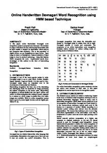
1.3. Computational Theories and Algorithms The investigation reported in this dissertation was conducted using the three-level methodology of a computational theory that is discussed in [Marr 1982, Chapter 1] and outlined in Figure 1.1. It was emphasized that perceptual processes should be studied separately on each of these levels. Each of the levels reinforces the others and they are logically and causally related, but there is only a loose connection between levels. The level of the computational theory is the most important. It provides the basis on which the other levels are built. In the computational theory of a process, ‘‘the performance of the device is characterized as a mapping from one type of information to another, the abstract properties of this mapping are defined precisely, and its appropriateness and adequacy for the task at hand are demonstrated.’’ The idea of a computational theory is well-illustrated by a cash register (from [Marr 1982, pp. 22-23]). Addition is what is computed by a cash register since a cash register combines prices to determine the total cost of a group of items. Why addition is used rather than some-
Computational Theory What is the goal of the computation, why is it important, and what is the logic of the strategy by which it can be carried out? Representation and Algorithm How can this computational theory be implemented? In particular, what is the representation for the input and output, and what is the algorithm for the transformation? Hardware Implementation How can the representation and algorithm be realized physically?
Figure 1.1. The three levels at which an machine carrying out an information processing task must be understood (from [Marr 1982, p. 25]).
6
CHAPTER 1
INTRODUCTION
thing else like multiplication are the constraints of the problem in the real world: 1.
Buying no items costs no money.
2.
The order in which the prices of items are entered into the cash register does not affect the amount of money paid.
3.
Separately paying for groups of items costs the same as paying for all the items at the same time.
4.
If after an item is purchased, it is returned for a refund, the total expenditure is nothing.
These real-world constraints specify the mathematical operation of addition. Constraint number 1 is analogous to the rules for zero, number 2 is commutativity, number 3 is associativity, and number 4 is the rule for inverses. Notice that the computational theory of the cash register has nothing to do with the algorithm for addition. At no time is the layout of the keyboard or the checkout stand mentioned, even though these are critical components in making a cash register actually function. The computational theory is detached from these concerns. It is formulated on a purely abstract level. The second level of representation and algorithm is the first time consideration is given to how the computational theory is implemented. A representation for the input and the output of the process is first chosen. For the cash register these are both base ten numbers. An algorithm is then chosen that carries out the operation specified by the computational theory. An algorithm for base 10 addition might be chosen. However, another algorithm might also be used. The choice could depend on some other considerations such as the hardware the algorithm is run on. It is very important to note that the computational theory is only loosely connected to
7
INTRODUCTION
CHAPTER 1
the algorithm. The third level of hardware implementation is where the nuts and bolts issues of how the algorithm is implemented are considered. The hardware implementation of an algorithm used by people might consider neurons and their connections. The hardware level implementation of a computer algorithm would consider gates and registers or maybe implementation on a VLSI chip. Again, the important point is that the hardware implementation is separate from the study of the algorithm, and the algorithm is separate from the computational theory. It is interesting to observe just how far the implementation level is from the computational theory. The separation of the levels cannot be stressed enough. It is important in studying a process that they do not become confused. For example, in formulating the computational theory of the cash register, the algorithm for implementing the theory was not a consideration. This is significantly different from attacking the problem all at once and simultaneously determining what a cash register should compute and how it should compute it. This would be similar to a novice programmer writing code without spending any time to understand what exactly the program should compute. Because the mechanism of a computational theory and its algorithm apply to any information processing task, and this methodology has enjoyed success in other domains, most notably the recovery of shape from images, it is chosen as the vehicle for the present investigation of reading. It will be seen that previous reading algorithms have lacked a solid theoretical background in human performance. This has led to the development of algorithms that have good performance in restricted domains but lack general purpose perceptual capabilities. By developing a computational theory for reading based on human performance it will be shown that the algorithms that implement portions of the theory have the capability of reaching levels of human competence.
8
CHAPTER 1
INTRODUCTION
The computational theory of reading will be based on previous studies of human performance. It will show what is computed by people when they read, why this is important, and general guidelines of how this should be carried out. Since reading is a complex information processing task involving interactions of knowledge from many different sources, algorithms will be developed that implement only a subset of these interactions. However, these algorithms will be sufficient to illustrate that if the complete version of the theory were implemented, a robust ‘‘reading machine’’ would result that would possess human fluency. In line with the relationships between a computational theory and its algorithms, the methods the algorithms use to compute their results will most likely be very different from the methods used by people. In this way, the algorithms will be different from a psychological simulation of reading. This is quite appropriate since the objective of this work is to develop algorithms that read digital images of text with a computer. Therefore, the algorithms should take advantage of their domain rather than being tailored to some other domain, such as the human processor. However, the algorithms must still compute what is specified by the computational theory.
9
INTRODUCTION
CHAPTER 1
1.4. Objectives of this Approach The primary objective of this dissertation is to illustrate that with a firm theoretical background based on how people read, a robust algorithm for reading text can be realized. The mechanism of this investigation is a computational theory and algorithm. This is used because reading is an information processing task that is suitable for this approach. Also, the reading problem is one that has lacked a method to incorporate knowledge about cognitive processing. This is true even though an immense amount of work has been done on the understanding of human reading. The insights yielded by studying human reading and applying the results to the development of new algorithms will be shown to result in techniques that are different from previous approaches. Previous approaches did not consider the entire reading problem and instead concentrated on specific visual processing aspects. Therefore, these methods worked well in the domains they were designed for but lacked provisions for expansion to the larger domain of unrestricted text.
10
CHAPTER 1
INTRODUCTION
1.5. Outline of the Dissertation The remaining six chapters of this dissertation discuss background, define the proposed approach, and discuss in detail three portions of a reading algorithm. This is followed by a chapter that summarizes results and conclusions, and discusses future work. The background discussion of chapter 2 concentrates on one theme: that reading algorithms and explanations for human reading are intimately intertwined and one should be studied in concert with the other. Therefore, several different approaches that have been taken in developing reading algorithms are surveyed. These are paralleled with some remarkably similar developments in explanations for human performance. Some portions of the human reading process are pointed out that should be included in a reading algorithm. Chapter 3 presents a computational theory and an algorithmic framework that integrates these processes. Three components of reading are chosen for implementation as the basis of an approach that is expandable to completely fluent reading. These components are hypothesis generation, hypothesis testing, and comprehension processes. Chapter 4 discusses hypothesis generation in detail. This is the generation of hypotheses about the identity of a word from a gross visual description. A method of doing this is proposed and a series of statistical studies are conducted to show the ability of this approach to produce a small number of hypotheses about the identity of a word that comes from a large vocabulary. The tolerance of this method to many different input formats is shown by experimentation with lower case, upper case, and mixed case text. Chapter 5 discusses a method of hypothesis confirmation that uses the words provided by the hypothesis generation stage of the algorithm to determine a strategy of hypothesis testing that discriminates between the hypotheses. This strategy is a series of feature tests that are executed on an input image. The tests discriminate between a limited number of features
11
INTRODUCTION
CHAPTER 1
determined by the hypotheses and are designed to be tolerant of the segmentation of the input word into characters. The result of hypothesis confirmation is either a recognition of the input word or a small set of hypotheses that contain it. The ability of hypothesis confirmation to do this reliably with a small number of tests is explored in a series of statistical experiments. An implementation is presented that demonstrates the operation of hypothesis confirmation on a database of word images. Chapter 6 discusses several comprehension processes and points out their potential contributions to the accuracy of a reading algorithm. Statistical studies are conducted to show the actual contributions of several of these processes to the reading algorithm. Chapter 7 summarizes the approach presented in this dissertation and the results derived from this work. Future work in this area is also presented.
12
Chapter 2 BACKGROUND
Algorithms for reading text and related theories of human performance are surveyed. Several different approaches to the machine reading problem are discussed and contrasted with similar developments in models of reading by people. These approaches include reading by isolated character recognition, reading by coupling character recognition with information from a dictionary of allowable words, and reading by recognizing entire words without using a technique that interprets individual characters. The commonalities that exist between algorithms that are structured in these ways and theories of human reading are pointed out. Instances are discussed where similar conclusions were independently reached in the human and machine reading domains. Areas of research in human reading are also pointed out that could be gainfully applied to the development of reading algorithms so that they might recognize a wider variety of fonts, scripts, and input styles than is currently possible.
13
BACKGROUND
CHAPTER 2
2.1. Introduction The reading of text by computer is a topic that has been investigated for many years. The objective of work in this area is to develop the ability to convert an image of machine-printed, hand printed, or handwritten text in a specific language into a computer-interpretable form, such as ASCII code, with the same fluency and accuracy that a person who was a skilled reader in that language would exhibit. This problem area has been the subject of intense research over the years; at least one patent dates back to 1931 [Weaver 1931] and another to 1935 [Maul 1935]. Some examples in the academic literature are Harmon’s early work on cursive script recognition [Harmon 1962], Munson’s as well as Duda and Hart’s work on the recognition of hand-printed text [Duda and Hart 1968, Munson 1968], and Bornat and Brady’s work on the organization of knowledge sources in a reading algorithm [Bornat and Brady 1976]. The academic interest in reading algorithms stems in part from a desire to discover an algorithmic solution to a problem that is solved with seemingly little effort by humans. The level of interest in this problem is shown by its use as a demonstration domain for many elegant algorithmic techniques such as error correcting tree automata [Fu 1982], graph-theoretic shape decomposition [Shapiro 1980], unsupervised
learning
[Niemann
and
Sagerer 1982],
and
hierarchical
relaxation
[Hayes, Jr. 1979, Hayes, Jr. 1980]. The commercial interest in reading algorithms is caused by the need to use computerized techniques to manage printed text. Successful commercial applications of reading technology1 include magnetic ink character recognition for bank checks, bank transaction slips [Spanjersberg 1978], postal order cards [Kegel et al. 1978], and the low-cost recognition of a few fonts of typewritten characters [Stanton and Stark 1985]. These are all specialized domains in which 1
14
An interesting study of early commercial reading technology is [Auerbach Publishers 1971].
CHAPTER 2
BACKGROUND
input format and font can be controlled. Other machines recognize a larger number of type fonts by requiring an operator to conduct a training session for new fonts [Ulick 1984]. Postal address reading machines, that are required to cope with a wider range of typestyles and formats than such specialized equipment, have been in use for over 20 years. However, even this equipment, which costs about $500,000 per machine, is only able to correctly read about 50 to 60 percent of the mail presented to it. Therefore, even machines such as these, which have been the subject of intense development effort by many companies, are far from being able to read the unconstrained texts that appear on an envelope with 100 percent accuracy [Hull et al. 1984]. Currently, the most common design of a reading algorithm (used by most of the commercial equipment discussed above) has the three stages shown in Figure 2.1a. The image preprocessing stage determines which areas of the image are text and isolates images of individual characters within the words of the text. These character images are then passed to a character recognition algorithm that identifies one or more letters that match each character. These decisions may then be passed to an optional contextual postprocessing algorithm that uses dictionary of words that can occur in the input text to resolve ambiguities or correct errors in the character decisions. There are some exceptions to this one-directional flow, most notably the Dictionary Viterbi Algorithm [Srihari et al. 1983]. Figure 2.1b shows the design of a word recognition algorithm wherein aspects of character recognition and contextual postprocessing are combined and whole words of text are recognized. This approach segments a word but the decisions for classifying each segment take into account the adjacent segments or their character classifications. Typically, this class of algorithms is applied to cursive script recognition, e.g., [Farag 1979]. However, it could be applied to discrete printed text as well. The following sections of this chapter survey the entire spectrum of reading algorithms. The basic strategy of each area is discussed and several notable approaches to each one are
15
CHAPTER 2
BACKGROUND
2.2. Character Recognition Character recognition techniques associate a symbolic identity with the image of a character. These algorithms operate on isolated character images that are usually thresholded, sizenormalized, and placed in a standard grid. These methods are generally classified as either template matching or feature analysis algorithms. Good surveys of character recognition techniques include [Suen et al. 1980] which is specialized for hand-printed characters and [Ullmann 1982] which covers commercial techniques.
2.2.1. Template matching Template matching techniques directly compare an input character image to a stored set of prototypes. The prototype that matches most closely provides recognition. In an early template matching approach the comparison was carried out optically [Hannan 1962]. More recent digital techniques use distance measures between input and prototype images such as the Hamming distance (the sum of the exclusive-or in a pixel-by-pixel comparison of the two binary images). A recent technique for template matching that avoids a pixel by pixel comparison between the input and all prototypes is based on a decision tree comparison procedure [Casey and Nagy 1984]. Decision tree methods reduce the computation in the comparison process with a sequential testing procedure [Moret 1982]. Tests that are more powerful than others are carried out first and their results determine the ordering of later tests. This is pertinent to template matching for character recognition since certain pixels in some characters are more likely to be black than the same pixels in other characters. Therefore, those pixels are tested first and the results of those tests are used to determine which pixels are tested next or if a recognition decision or a rejection is output.
17
BACKGROUND
CHAPTER 2
An example of a decision tree for discriminating between ‘‘A’’, ‘‘B’’, and ‘‘C’’ is presented in Figure 2.2. The pixels in a 10x10 character frame are numbered as shown in Figure 2.2(a) and three prototypes are shown in Figure 2.2(b). The location of pixel in row i and column j is designated (i,j). Given an unknown input from among the three prototypes, the decision tree in Figure 2.2(c) specifies that pixel (4,1) is tested first. If it is white, the input is classified as an ‘‘A’’, otherwise, pixel (1,1) is tested. If it is white, the input is rejected since no prototype with a black pixel at (4,1) has a white pixel at (1,1). On the other hand, if pixel (1,1) is black, pixel (5,6) is tested. If it is black, the input is classified as a ‘‘B’’ otherwise it is classified as a ‘‘C’’. The storage and computational efficiency of a decision tree system for template matching is illustrated by this simple example. Only three internal nodes and four terminal nodes were needed for the tree. In a compressed format, 6 bits could represent each of the three nonterminal nodes. This is done by encoding the seven possible descendents of any node with a three-bit pattern. (The seven descendents are the three non-terminal nodes and the four decisions.) Thus, a total of 18 bits are needed to store the tree. This is only 6% of the 300 bits needed to store the three 10x10 prototypes. Also, at most three pixels have to be examined to make a classification. This is much better than the 3*10*10=300 operations needed for a brute force implementation of the Hamming distance. Further economy could be achieved if the (1,1) node were deleted from the tree. It is retained in this example to illustrate the use of a reject option. The design of a document reading system is discussed in [Wong et al. 1982] in which a decision tree method is used to match input characters with prototypes. An implementation of this technique used three decision trees to represent a training set of about 500 samples of each of 85 typewritten symbols from the the Courier-10 font [Casey and Jih 1983]. Each tree con-
18
BACKGROUND
CHAPTER 2
tained 2000 nodes and was designed to examine different sets of pixels. Only 36 kilobytes of storage were required. Out of a test set of 208,450 characters, only ten were rejected and five misrecognized. This is a recognition rate of almost 100 percent. Reading rates of several hundred characters per second were projected for a commercial implementation of this methodology. The strengths and weaknesses of a decision tree implementation of template matching are illustrated by this method. It is reliable, fast, and requires little storage. However, it is only suitable for simultaneous application to at most a few fonts. It is also sensitive to registration of the input and noise in the image. Therefore, it is probably not very useful as a general purpose reading algorithm.
Parallel to Human Performance The parallel between reading algorithms and explanations for human reading has an interesting footnote in template matching. It turns out that template matching has been proposed as the method people use to recognize characters [Smith 1982]. This is a wholistic or gestalt theory of perception which asserts that a single prototype exists in the mind of an individual for every letter and that these prototypes are matched to input letters to determine recognition. However, this explanation is untenable since no single template can describe the wide variety of characters that are easily perceived by a human reader [Neisser 1967]. Figure 2.3 illustrates this point with many examples of the letter ‘A’ that would have to correspond to a single mental template for the theory to be plausible.
20
BACKGROUND
CHAPTER 2
2.2.2. Feature analysis Feature analysis algorithms for character recognition attempt to overcome the limitations of template matching and thereby capture some of the robustness of human letter reading. Instead of wholistically matching an input character to prototypes, feature analysis techniques use a two-step process in which a predefined set of features is first extracted from an input character. A classification algorithm then matches the resultant feature description to the stored feature descriptions of ideal characters. The class label of the best match is output. The extraction process implies that features have already been defined and algorithms have been developed to identify those features. Definition is done a-priori by the designer of a system and is based on many considerations including the ability of the features to capture differences between characters, as well as the accuracy with which the features can be calculated. Extraction involves the execution of image processing operations on the image of a character to determine the features2.
Feature Definition The definition of the features that are used is a critical step in any feature analysis algorithm. The smallest number of features should be used that describe the differences between characters and can be reliably extracted. Although some formal methods have been proposed for feature selection in character recognition, e.g., [Stentiford 1985], intuition is still the primary technique utilized. In [D’Amato et al. 1982, Stone et al. 1986] the contour of handprinted characters is analyzed for the presence of features such as loops, arcs, etc. In [Lai and Suen 1981] a technique is proposed that combines boundary analysis with fourier shape description. Pavlidis presents a method in which over 100 features are extracted from the 2
22
The reader is referred to [Ballard and Brown 1982] or [Pavlidis 1982] for textbooks that cover this topic.
CHAPTER 2
BACKGROUND
skeleton of a character [Pavlidis 1983]. Duerr et al. discuss a system that combines boundary and topological features [Duerr et al. 1980]. The systematic determination of a non ad-hoc feature set was explored by Shillman [Shillman 1974, Shillman et al. 1976, Shillman and Babcock 1977]. Based on the observation that humans are quite good at reading isolated characters, Shillman sought to discover the features people use for this task. He conjectured that if those features were used by a character recognition algorithm then it should perform as well as a human reader. He distinguished three attributes of a feature: physical, perceptual, and functional. Figure 2.4. presents a diagram (adapted from [Blesser et al. 1974]) that illustrates the differences. The physical attribute of a feature refers to its presence or absence in the image. For example, the ‘‘O’’s in Figures 2.4(b)-(d) are physically open because in each case there is a connected path of white pixels from the background to the cavity in the middle. The perceptual attribute of a feature expresses how a person perceives its presence or absence. In Figures 2.4(a) and 2.4(b) the ‘‘O’’ is perceptually closed even though in 2.4(b) it is physically open. The functional attribute of a feature describes its state with respect to the classification of the character. For example, the ‘‘O’’ of Figure 2.4(c) is functionally closed because the character image is identified as an ‘‘O’’. This is true even though the image is both physically and perceptually open. Shillman postulated that the feature description of a character used in a recognition algorithm should be based on functional attributes rather than physical attributes, as is commonly done. This would provide a description scheme that is invariant to a wide variety of distortions. Twelve functional attributes were identified: Shaft, Leg, Arm, Bay, Closure, Weld, Inlet, Notch, Hook, Crossing, Symmetry, and Marker. Each functional attribute was further described by up to four modifiers (location, orientation, segmentation, and concatenation). The recognition of a functional attribute was done by first detecting a physical attribute and mapping it onto the
23
CHAPTER 2
BACKGROUND
corresponding functional attribute by means of a physical to functional rule (pfr). The parameters of the pfr’s were determined by a psychological procedure in which a series of letters with different values of the same physical attribute were presented to subjects. Their judgements determined the presence or absence of a particular functional attribute as well as the allowable variance in the physical attribute. An example physical-to-functional rule derived by this procedure is: If
the ratio of the size of a gap on the right side of a character to its height is less than 0.23,
then the right side of the character is functionally closed. This methodology was demonstrated with a feature set that differentiated between handprinted ‘U’s and ‘V’s [Suen and Shillman 1977]. This is one of the more difficult problems in isolated character recognition. A correct recognition rate of 94% was achieved on the Munson database of hand-printed characters [Munson 1968]. This was better than human performance on the same data. An extension of the Shillman method was developed by Cox et al. [Cox, III et al. 1982] who added a skeletal level between the functional and physical levels. The purpose of this intermediate level was to provide two capabilities not easily incorporated in the original pfr method. First, the ability to discriminate between letters and non-letters was needed since, for example, any blob that satisfied the above pfr would be given the functional attribute of right closure. Second, the representation of stylistic constraints, such as serifs, was provided for. This second capability was especially important for the application of this representation to the generation of character images. It was observed that the skeletal descriptions would provide a degree of robustness to character recognition if mappings were provided from the physical to skeletal levels and from the skeletal to functional levels. 25
BACKGROUND
CHAPTER 2
Feature Classification The classification of the feature description of a character is usually done with either a statistical or a syntactic technique3. The paradigm statistical classifier maps the features that are extracted from a character image onto a feature vector with components that are either binary, integers, or real-valued. Thus, a character image is reduced to a point in a multi-dimensional feature space. A discriminant function is then used to map a feature vector onto a list of values, one for each of C classes, where the highest value corresponds to the class that is most similar to the input. The discriminant function may be given a-priori, or it may be estimated from a pre-classified set of samples during a training phase. A testing phase may then be used to validate the classifier during which time its performance on sample data is observed. The classifier is accepted for operational use if its level of performance is judged to be adequate. A survey of statistical methods for character recognition is given in [Nagy 1982].
An interesting
classification technique that has been used for character recognition is that of neural networks [Fukushima 1986]. One approach to the estimation of a discriminant function that has enjoyed commercial success is described in [Doster 1977] and [Schurmann 1978]. In this method, an n x n binary character image is mapped onto an N-element vector where each element is obtained by combining a selected pair of pixels. The vector size, N can be as large as
n2 + n 2 + 1, however, a 2
much smaller, heuristically chosen value, is typically used. The discriminant values are then computed from this vector by multiplying it by an NxC matrix of coefficients that was determined during a training phase. In the implementation reported in [Doster 1977], n=16, the maximum value of N was 32,897, and a value of N=1200 was used in practice. A problem with 3
26
The reader is referred to [Duda and Hart 1973] or [Fu 1982] for textbooks on these subjects.
CHAPTER 2
BACKGROUND
this approach is its requirement for a large number of samples to determine a coefficient matrix that can reliably recognize a wide range of characters (over 100,000 samples are reported in [Schurmann 1978]). However, this method is reportedly very robust. A more recent version of this methodology uses a hierarchical approach in which successive classifications into smaller hypothesis sets is performed until a small, ranked set of decisions is achieved. This has the advantage of improved performance at lower computational cost as well as suitability for micro-processor implementation [Schuermann and Doster 1984]. Syntactic or structural approaches to feature vector classification do not rely on statistical decision rules. Instead, an input character is described as a composition of some basic pattern primitives and this description is parsed according to a description of allowable compositions. The output of the parse is either the class to which the input belongs or a rejection. Allowable descriptions can be given in terms of a grammar at any of the four levels in the Chomsky hierarchy (regular, context-free, context-sensitive, or unrestricted). Regular grammars are often quite adequate for character recognition, e.g., [Duerr et al. 1980], although the power of the other techniques is sometimes helpful, e.g., the context-free tree grammar of [Agui et al. 1979], or the context-sensitive grammar of [Stringa 1978]. The syntactic method described in [Ali and Pavlidis 1977, Pavlidis and Ali 1975, Pavlidis and Ali 1979] is a good example of a syntactic approach to character recognition that uses a regular grammar. This method analyses a character image in two steps. First, a piecewise linear approximation of the contour is decomposed into a sequence of arcs and each arc is described by several features, including its convexity or concavity, its direction (either North, Northeast, East, Southeast, South, Southwest, West, or Northwest), its vertical location, its horizontal location, and its length. The concatenation (around the contour) of arc descriptions is then parsed by a finite automaton. The state the finite automaton is in when the input is exhausted deter-
27
BACKGROUND
CHAPTER 2
mines the classification. A description of the finite automaton (called a ‘‘prototype description’’) that recognizes a ‘3’ follows:
(1)
Any number of arcs, followed by:
(2)
A concave arc facing West in the bottom middle or bottom right of the character, followed by:
(3)
Any number of arcs, followed by:
(4)
A concave arc facing West in the top half of the character, followed by:
(5)
Any number of arcs that do not include an arc in the lower right of the character that faces East.
43 such prototype descriptions were constructed by observation of the output of the decomposition process when run on a training set of 480 handwritten numerals. More than one prototype description was allowed per class. A recognition rate of 93% with an error rate of about 4% and a rejection rate of about 3% were achieved on a testing set of 840 handwritten numerals.
Parallels to Human Performance The parallels of feature analysis algorithms for character recognition with human performance are most interesting. Indeed, feature analysis has been adopted as the best explanation for human character recognition [Neisser 1967]. This is because of the ability of feature analysis to deal with the differences in input format, etc. that are needed to account for the human ability to read almost an infinite variety of printed matter. The definition of the features used by human readers is a critical part of research in this area just as it is in determining the performance of a character recognition algorithm. Haber and Haber identified four techniques that are commonly used to discover the features people use to recognize characters [Haber and Haber 1981]. The first of these methods relies solely on the intuition of a single experimenter and the last three use experimental data from human subjects to reinforce the choices made by an experimenter. The first technique for feature definition is the armchair method in which an 28
CHAPTER 2
BACKGROUND
experimenter determines the minimum feature set that describes the differences between characters; an excellent example of which is presented in [Haber and Haber 1981]. The second technique for defining a feature set is for an experimenter to manipulate the visual characteristics of letters to determine those features that differentiate letters, thereby identifying features that, presumably, are important to recognition. This is basically the method used by Shillman [Shillman 1974]. The third technique uses judgements by subjects about between-character similarity to enforce an intuitive choice of features by an experimenter [Dunn-Rankin 1968]. The fourth method uses the pattern of errors made by subjects in a recognition task to construct a confusion matrix (an example of such an analysis is [Townsend 1971]). Features are then tested for their validity by the data in the matrix. This is done by observing the percentage of time a given letter is recognized as another letter with the same feature. The higher this percentage, the better is the feature for explaining the responses of the subjects.
For example, in
[Bouma 1971], when tall letters are presented, 92% of all responses were tall letters. The complete set of features for lower-case characters determined in [Bouma 1971] are presented in Table 2.1 along with the characters that possess those features. The third column presents the set of stimuli that possess the feature given in the second column. In most cases the set of correct responses (the same or other letters that also possess that feature) is identical to the set of stimuli. In those cases where the set of correct responses contains some other letters, this augmented set is shown next to the set of stimuli. The process by which people recognize characters (the human character recognition algorithm) has not been the subject of nearly as much attention as the definition of features or the development of recognition algorithms. However, some recent work sheds some light on this subject. Lupker identified a hierarchical process of character recognition in which people first acquire information about the gross shape of a character and more slowly acquire information
29
BACKGROUND
CHAPTER 2
���������������������������������������������������������������������������������� ����������������������������������������������������������������������������������� no. Feature Stimuli, Correct Responses Percent Correct Responses � � � Short letters { a,c,e,m,n,o,r,s,u,v,w,x,z } 84 � (1) � Tall letters { b,d,f,h,i,k,l,t,g,j,p,q,y } 92 � (2) � � (3) � Short and rectangular { a,s,z,x,n,m,u } 65 � (4) � Something inside short letter { a,s,z,x,e,m,w } 60 � � Round { e,o,c } 63 � (5) � Left part round { e,o,c },{ e,o,c,d,q,a,g } 74 � (6) � Right gap { e },{ e,c,s,z,x,r,t,f } 38 � (7) � � (8) � Right gap, no inner part { c },{ e,c,z,x,r,t,f } 66 � (9) � Two vertical outer parts { n,m,u },{ n,m,u,h } 77 � � Lower gap { n },{ n,m } 80 � (10) � Upper gap { u },{ u,v,w } 65 � (11) � Obliques { v,w } 92 � (12) � � (13) � Left upper extension { h,k,b } 89 � (14) � Right upper extension {d} 88 � � Slender letter { t,i,l,f,j } 90 � (15) � (16) Upper Dot { i },{ i,j } 70 ����������������������������������������������������������������������������������� � Table 2.1. Bouma’s features for lower case characters [Bouma 1971].
about its finer details [Lupker 1979]. This is similar to Taylor’s bilateral cooperative model of reading [Taylor 1984]. It is also similar to hierarchical algorithms for character recognition by computers such as [Gu et al. 1983, Schuermann and Doster 1984, Sridhar and Badredlin 1984]. A problem with all the methods for feature definition and the modeling of character recognition mentioned above is that each one requires an experimenter to pick the features or set up the model. There is no way to be sure a particular feature is used a particular way. The best that can be achieved is a confirmation of the experimenter’s choices by the performance of subjects. Also, the isolated character recognition task used to carry out this confirmation is significantly different from the usual reading situation. Thus, the features and recognition strategies determined by these procedures may have little relevance to normal human reading. This is
30
shown
in
studies
such
as
[Balota
and
Rayner 1983, Becker 1985, Dennis
et
CHAPTER 2
BACKGROUND
al. 1985, Fisher 1975] where many factors such as visual context, surrounding letters, phonology, and different syntactic and semantic content influence the reading process and its attendant feature testing strategy.
Therefore, reading algorithms probably incorporate additional
knowledge, beyond that available from isolated character images. One such knowledge source is a dictionary or list of words that could occur in an input text.
31
BACKGROUND
CHAPTER 2
2.3. Contextual Postprocessing Contextual postprocessing techniques use a dictionary of words to detect and sometimes correct errors in the output of a character recognition algorithm. These errors are most often the substitution of an improper character for the correct one, the merger of two adjacent characters (sometimes called a deletion error), or the splitting of one character into two (producing an insertion error). Merges and splits are caused by improper segmentation during preprocessing. Substitution errors are caused by an error in the recognition process. Some contextual postprocessing techniques take as input a fixed string of hard decisions output by a character recognition algorithm. These are sometimes referred to as spelling correction techniques since they are sometimes applied to the correction of spelling errors in an office automation environment as well as the correction of recognition errors4. Other more general contextual postprocessing algorithms use information about the reliability of the decision of a character recognition algorithm. This usually leads to increased accuracy at decreased cost. For example, a spelling correction algorithm might be presented with the string ‘‘qvit’’ and in a similar situation a character recognition algorithm might provide the additional information that ‘‘u’’ was a highly rated candidate for the second position. To correct this error, the DEC-10 SPELL spelling correction algorithm would substitute the other 25 letters in every position and make a decision only if a single such word was found in a dictionary [Peterson 1980]. An operator would have to make the final decision if more than one candidate was located. In contrast, the contextual postprocessing technique discussed in [Doster 1977] would capitalize on the ranking information by doing a similar substitution and lookup only for each ranked character alternative. It also uses the likelihood values associated with each ranking to compute a figure of merit for each candidate word. It outputs the most highly ranked candidate 4
. The reader is referred to [Peterson 1980] for an excellent survey of spelling correction algorithms.
32
CHAPTER 2
BACKGROUND
it finds in the dictionary. In the above example up to 101 dictionary accesses would be required for the spelling correction technique but only two would be needed for the contextual postprocessing algorithm. Contextual postprocessing algorithms also differ in the way they represent the dictionary. Some use an approximate representation for a dictionary, such as probabilities of letter-tuples or n-grams [Shinghal and Toussaint 1979b], and others use an exact representation, such as a hash table [Shinghal and Toussaint 1979a], that represents complete words. Methods that use an approximation can only output strings of letters that obey the rules implicit in their approximation. These letter strings are not necessarily legal words. However, approximation-based techniques are usually computationally more efficient than methods that use an exact representation wherein a legal word is the guaranteed output.
2.3.1. Approximate dictionary representations Probabilities of letter-pairs or letter-triples (called letter transition probabilities) have frequently been used to approximate a dictionary [Morris and Cherry 1975]. The reason for this is the high degree of redundancy reflected in these probabilities. For example, in the over one million word Brown corpus, only 64% of the 676 possible pairs of letters ever occur and only 55% of the letter pairs occur more than 0.002 percent of the time [Kucera and Francis 1967, Suen 1979]. The potential usefulness of this information is also indicated by the low information content or entropy in a typical text [Shannon 1951]. For example, it was estimated that an average of 1.3 bits are needed to encode each of the 27 symbols in an English text [Cover and King 1978]. This is much less than the maximum of log227 = 4.755 bits per character. It was stated that this implies English is 64% redundant, i.e., 64% of the letters in the original text could be deleted and the original could be reconstructed from what remains.
33
BACKGROUND
CHAPTER 2
The redundancy of English, as reflected by the sparceness of the transition probability arrays, is capitalized on by the binary n-gram algorithm for contextual postprocessing [Hanson et al. 1976, Riseman and Hanson 1974]. This method assumes an input word is contained in a fixed vocabulary and quantizes non-zero probabilities as 1’s (indicating the presence of that ngram somewhere in the vocabulary) and zero probabilities as 0’s (indicating the absence of that n-gram). Typically, digrams (letter pairs) or trigrams (letter triples) are used in this technique. A binary n-gram array has n dimensions and 26n storage locations. Each dimension may also be parameterized by n position indices. An example definition of such a positional binary digram array Bijn , where i and j are the position indices of the array, is:
Bijn (α,β)
=
⎡ 1 if letter α occurs in position i and letter β ⎪ occurs in positionj of some dictionary word; ⎪ ⎣ 0 otherwise.
Many varieties of these arrays can be defined. If the n position indices refer to any n adjacent positions, then only one non-positional array is used to describe a given fixed vocabulary. When the position indices refer to n specific, adjacent locations, there are (maxwl) different nn gram arrays, where maxwl is the number of letters in the longest word. If the vocabulary is divided into subdictionaries by word length (wl ) and the n-gram arrays are further parameterized by wl , there are ⎧ ⎫ (wl) = ⎪maxwl +1 ⎪ n ⎩ n +1 ⎭ wl =n
maxwl
Σ
different n-gram arrays. Many other arrangements are also possible. The one that is used depends on the storage available and the goal of the application [Hull and Srihari 1982b, Hull and Srihari 1982a].
34
CHAPTER 2
BACKGROUND
The binary n-gram algorithm detects whether an input word contains one or more errors by retrieving all the pertinent n-gram entries. If they are all ‘‘1’’ the input word is considered legal and if any n-gram is ‘‘0’’ the input is known to contain an error since it contains an ngram not in the vocabulary. Note that since an approximate dictionary representation is used, it is possible for an error to occur but for all the pertinent n-grams to be ‘‘1’’. This would occur if an error produced n-grams that were contained in some other word(s). However, it is not possible for a correct word to produce an n-gram not in one of the n-gram arrays because of the assumption that only words from a fixed vocabulary are input to the character recognition algorithm. The correction of words with errors uses a fixed decision strategy. A substitution error is first assumed to have occurred and its correction is attempted. If this works out, the corrected word is output and the correction process terminates. Otherwise, the correction of a split error, a merge error, and a transposition error are attempted, in that order. If none of these corrections can be performed, the input word is rejected. It should be noted that this strategy could be modified in many ways, e.g., to correct only single substitution errors. The correction of a single substitution error can utilize positional binary n-grams. If an input word contains an error, the position indices of the n-gram arrays that returned 0 are intersected. If no position index occurs in the result, the hypothesis of a single substitution error must be false. This phase of the correction process is then terminated and control is returned to the decision procedure. If only one position index occurs in the result of the intersection, a vector is extracted from each n-gram array that involves that position. These vectors are then intersected and if there is a single ‘‘1’’ in the result, the letter corresponding to its location is substituted in the position that contained the error. The resultant word is output. If the position of a single substitution error cannot be uniquely determined, i.e., there was more than one element
35
BACKGROUND
CHAPTER 2
in the intersection of position indices, correction is attempted for each such position, as above. If only a single correction is found, that word is output. Otherwise, the input is rejected. An example of the operation of the binary n-gram algorithm is shown in Figure 2.5. A dictionary of three three-letter words { cat, cot, tot } and the three positional binary digram (n=2) arrays derived from this dictionary are shown, as are examples of the error detection and correction processes. If a character recognition technique output the string ‘‘coo’’, detection of the error would be done by: d 1,2(c ,o )
∩
d 1,3(c ,o )
∩
d 2,3(o ,o ).
This returns a 0 from both d 1,3 and d 2,3. Since the intersection of {1,3} and {2,3} yields {3}, error correction is done by intersecting the vectors: d 1,3(c ,* )
∩
d 2,3(o ,* ).
where the position of a ‘*’ indicates that the vector varies over that dimension of the array. The resulting vector has only one non zero element, corresponding to a ‘‘t’’ Therefore ‘‘coo’’ is corrected to ‘‘cot’’. This short example illustrates several of the advantages and disadvantages of this method. The computations to locate and correct errors are relatively simple and involve only binary comparisons. Hence, they can be economically implemented. However, the potential storage costs are also apparent by observation of the sparceness of the arrays. This is a major weakness of this method, as discussed in [Hull and Srihari 1982b], where the binary n-gram technique was compared to an approach that uses an approximate, statistical representation of a dictionary. The binary n-gram method was shown to be good for error detection, however, the statistical approach was better for error correction. This was due in part to the large amount of memory needed to yield good correction performance with the binary n-gram method.
36
CHAPTER 2
BACKGROUND
dictionary: { cat, cot, tot }
a c o t
�
a c o t ����������������
�
� 0 0 0 0 � � 1 0 1 0 � � 0 0 0 0 � � 0 0 1 0 � ������������������
a c o t
�
a c o t ����������������
�
� 0 0 0 0 � � 0 0 0 1 � � 0 0 0 0 � � 0 0 0 1 � ������������������
d 1,2
d 1,3
a c o t
a c o t ���������������� � � � 0 0 0 1 � � 0 0 0 0 � � 0 0 0 1 � � 0 0 0 0 � ������������������ d 2,3
input word: ‘‘coo’’
error detection: d 1,2(c ,o )
∩
d 1,3(c ,o )
∩
d 2,3(o ,o ).
error correction: 1. position determination: { 1,3 } ∩ { 2,3 } = { 3 } 2. correction: d 1,3(c ,* ) ∩ d 2,3(o ,* ) = [00000000000000000100000000]. output word: ‘‘cot’’.
Figure 2.5. An example of the operation of the binary n-gram algorithm. A dictionary and its representation by positional binary digram arrays are shown, as is an example of the error detection and error correction processes of the algorithm.
37
BACKGROUND
CHAPTER 2
The correction of other types of errors with the binary n-gram technique is more fully discussed elsewhere [Fisher 1976]. Modifications that detect and correct words that contain up to two errors have also been developed [Ullmann 1977]. The frequencies of letter n-grams were exploited in the program discussed in [Morris and Cherry 1975]. This method used the frequency of letter triples to signal incorrect words in a spelling correction algorithm. Raviv adopted the formalism that English text was a Markov source and used character transition probabilities to postprocess text output by a character recognition algorithm [Raviv 1967]. A similar approach was used by Donaldson and Toussaint [Donaldson and Toussaint 1970]. The Viterbi algorithm [Forney 1973] is a statistical technique for decoding signals that was suggested as a contextual postprocessing algorithm by Neuhoff [Neuhoff 1975]. Srihari presents an excellent discussion of the application of the Viterbi algorithm to various problems [Srihari 1987]. The Viterbi algorithm models the production of the sequence of characters in a text as a Markov process. Under the assumptions that word delimiters (the blanks at the ends of words) are perfectly recognized and the occurrence of errors in a particular position is independent of the occurrence of an error in any other position, the Viterbi algorithm outputs the string of characters Z = z 0,z 1,...,zn +1 that maximizes Bayes’ formula: P (Z | X ) =
P (X | Z ) P (Z ) P (X )
2.1
where X = x 0,x 1,...,xn +1 is an input word and x 0 = xn +1 = z 0 = zn +1 = ‘ ′. The independence and Markov assumptions, as well as the fact that the maximization of equation (2.1) is independent of X reduces the maximization of (2.1) to the maximization of: n +1
Π P (Xi | Zi ) P (Zi | Zi −1) i =1
2.2
over all possible Z , where P (Xi | Zi ) is the conditional probability of the feature vector Xi 38
CHAPTER 2
BACKGROUND
taking on its value given that the corresponding input letter is Zi , sometimes called a ‘‘confusion probability’’, and P (Zi | Zi −1) is the first order transition probability of the occurrence of letter Zi given that the letter Zi −1 has been observed. To avoid the combinatorial explosion inherent in calculating equation (2.2) for all possible 26n strings Z , the Viterbi algorithm uses a dynamic programming formulation to transform the problem into one of graph searching with a computational requirement on the order of 262 operations. An example of the graph the Viterbi algorithm uses is shown in Figure 2.6. The concatenation of the letters on the nodes in each path from the node on the left to the node on the right represents a potential output string. The three letters ‘‘KDD’’ across the top of the figure represent an example output of a character recognition algorithm. The letters on the nodes are the alternatives for the input letter above them. The alternatives are determined by the character recognition algorithm. Only the five highest ranked alternatives are shown. The ranking is determined by the probability (determined by the character recognition algorithm) that the input character was confused with the letter on the node. The basic Viterbi algorithm that would operate on this graph is summarized:
39
CHAPTER 2
BACKGROUND
where, prev_cost and word are vectors of real values and strings, respectively, that have the same number of elements as there are rows in the graph. Prev_cost holds the accumulated costs of reaching the nodes in the previous column and word holds the strings of characters accumulated for nodes in the previous column. Max(temp,u) returns the maximum of the elements in temp with the side-effect that u is set to the index of the maximum element; concat(word[u],Z j ) returns the result of concatenating Z j on the end of word[u]. The algorithm operates one column at a time from left to right on this graph. The columns are numbered 0,1,...,Numchars+1, where Numchars is the number of characters in the input word. It computes the partial cost of reaching each node as the product of the previous cost and the applicable transition and confusion probabilities. This process is guaranteed to locate the best-cost path. The string of letters on the best-cost path is output from word[1] after the last iteration. Modifications of the algorithm for the sake of computational efficiency include using logarithms of probabilities and a summation rather than a product in the calculation of the cost. Other modifications use a fixed number of alternatives less than 26 [Shinghal and Toussaint 1979b], a variable number of alternatives determined by a threshold [Hull and Srihari 1982b], or a variable number of alternatives determined by the character recognition module [Doster and Schurmann 1980]. Even though this approach is computationally efficient, and can achieve relatively good performance, it may still output a string of letters that is not a legal word since it does not use an exact representation for a dictionary.
2.3.2. Exact dictionary representations Contextual postprocessing techniques that use an exact dictionary representation have spanned a wide range of sophistication. The simplest idea is to use a dictionary of legal words as an identity checker. If an input word is not in the dictionary, either a human operator decides
41
BACKGROUND
CHAPTER 2
the course of action, or a correction is attempted by some other means such as digram statistics [Cornew 1968]. A general class of techniques suitable for text error correction with an exact dictionary representation are known as string distance measures (SDM’s) [Hall and Dowling 1980] or Levenshtein distance metrics [Levenshtein 1966]. An SDM defines the distance between two words as the smallest number of substitutions, insertions, and deletions needed to transform one string into the other. This has been modified to provide variable weights for each class of error [Okuda et al. 1976]. An SDM is applied to contextual postprocessing by replacing an incorrect word by the dictionary word with the smallest distance. An SDM is applied to speech recognition in a similar way [Tanaka et al. 1986]. The computational problem of computing an SDM for every dictionary word was addressed by Kashyap and Oommen [Kashyap and Oomman 1981a, Kashyap and Oomman 1981b, Kashyap and Oommen 1984] who used a letter tree or trie to reduce the number of redundant computations and thus speed up the algorithm. Reuhkala presented a technique based on an SDM that used a hash table to retrieve a number of words that were similar to an input word [Reuhkala 1983]. The trie is an important data structure for contextual postprocessing techniques such as [Bozinovic and Srihari 1982]. First introduced by Friedkin [Friedkin 1960], the trie is a tree data structure that uses nodes to represent letters. The root has up to 26 descendents that correspond to the first letters in the words of a fixed vocabulary. Each of those nodes may have up to 26 descendents that represent the letters that may follow the letter of their ancestor in the vocabulary. This process is continued to as many levels as necessary to represent the longest dictionary word. Nodes that are the last letter in a word are so indicated. The trie was used in the dictionary viterbi algorithm (DVA) [Hull et al. 1983, Srihari et al. 1983]. This is a modification of the viterbi algorithm presented earlier. During the process
42
CHAPTER 2
BACKGROUND
of computing the cost of paths in the trellis, the presence of those paths in the trie are determined by the DVA. Only paths that are initial substrings of dictionary words are expanded further. This is incorporated in the Viterbi algorithm by adding a vector of pointers (prev_ptr) into the trie where there is one element for each initial substring of a dictionary word that is stored in the word vector. Step S1 in the algorithm presented before is changed to: if in_trie (prev_ptr[k], letter j ) then temp[k] := prev_cost[k] * P (XCol | Z j )*P (Z j | Zk ) else temp[k] := INFINITY ; Also, the vector trie_ptr is updated at the end of each j-loop: trie_ptr[j] := descendent( prev_ptr[u], letter j ); and trie_ptr is copied to prev_ptr before the next column is considered. This is a natural integration of both the Viterbi algorithm and a dictionary that retains the computational efficiency provided by Shinghal and Toussaint’s heuristic modification to the basic Viterbi algorithm[Shinghal and Toussaint 1979b]. A trie-driven approach for contextual postprocessing was suggested by Shapiro that uses the A* algorithm to find the dictionary word that best matches the input [Shapiro 1983]. The A* algorithm is a state-space search technique that locates the best-cost path in a graph from a source node to a goal node [Hart et al. 1968]. It includes a heuristic estimate of the cost of a path from any node to a goal node to improve efficiency. As long as this estimate is always less than or equal to the true cost, the best path is guaranteed to be found. In the case of contextual postprocessing with a trie and the A* algorithm, the source node is the root of the trie and a goal node is any node marked to indicate that it is the end of a word. In addition, the distance from the root to a goal node is equal to the number of letters in the
43
BACKGROUND
CHAPTER 2
input word. In an implementation constructed by the author, only substitution errors were considered. However, insertion and deletion errors could also be accommodated. The cost of a path was computed as the sum of the logarithms of the pertinent confusion and transition probabilities. The estimate of the cost to reach a goal node from a given node was computed as the sum of the pertinent number of the smallest confusion and transition probabilities. The transition probabilities were computed from a machine-readable version of Chapter 9 of [Winston 1977]. The confusion probabilities were developed from a model of a communication channel that introduced substitution errors. When tested on a corrupted version of the chapter mentioned above, the correction rate was 95% as opposed to 87% for the DVA. However, the DVA used less time than the A* algorithm. These two programs were both implemented in Pascal on a Vax-11/750 that was running the UNIX5 operating system. Thus, even though the A* algorithm finds the best choice for an input word (as the DVA was earlier thought to do), its time requirement may be excessive in practice.
5
44
UNIX is a trademark of Bell Labs
CHAPTER 2
BACKGROUND
2.4. Word Recognition Word recognition algorithms recognize whole words of text rather than composing word decisions from decisions about individual characters. This methodology avoids the error-prone segmentation step by extracting features without regard to the character in which they occur. Word recognition techniques are characterized by an integration of feature extraction and a dictionary. This is in contrast to the character recognition and postprocessing paradigm described earlier in which knowledge about a vocabulary is not used until after crucial decisions have been made. An implicit assumption of a word recognition algorithm is the presence of a dictionary, or list of words the algorithm might encounter. Although most implementations of word recognition approaches have been applied to cursive script recognition and have used dictionaries of 100 words or less (e.g., [Brown and Ganapathy 1980]), recent work has included experimentation with machine-printed text [Brickman and Rosenbaum 1982] and dictionaries of over 48,000 words [Hull 1985, Hull 1986a]. There are two basic designs for a word recognition algorithm. The first is a wholistic matching process in which an input word is compared to every word in the dictionary and the word that matches best is output. The second methodology is a hierarchical one in which a subset of a dictionary is first located that is similar to the input word. A disambiguation process is then executed that uses additional feature analysis to determine which member of the subset best matches the input word. Disambiguation is most often a bottom-up process in which a large number of features are extracted independently of the members of the subset. However, a topdown method has recently been developed in which the members of the subset determine the features that are extracted [Hull and Srihari 1986].
45
BACKGROUND
CHAPTER 2
2.4.1. Wholistic matching The word recognition technique that is part of the Word Autocorrelation Redundancy Match (WARM) technique for facsimile data compression is a good example of a wholistic method for reading words [Brickman and Rosenbaum 1982]. In this method, the top 150 most frequent words, that make up about 50% of a typical correspondence, are recognized by a twostage template matching process. The first stage determines a good preliminary correspondence between an input binary word image I and a prototype binary word image P by calculating a weighted sum of the exclusive-or between I and P :
Σ w 1(i ,j ) (I (i ,j ) c P (i ,j )), i ,j
(2.2)
where c is the exclusive-or operator. A black pixel is considered to have the logical value true and the numerical value 1. A white pixel is logically false and numerically 0. The weight w 1(i ,j ) is determined by the number of black neighbors N possessed by I (i ,j ):
���������� ����������� N w1 � � � 1 � � 0,1 3 � � 2 � 3 12 � ������������ 4 25 �� P is initially placed at the center of I and shifted by up to 2 pixels horizontally and vertically. The summation in equation 2.2 is calculated at each position. The position that yields the minimum sum is then used in the second stage of template matching. The second stage calculates almost the same summation as in equation 2.2 except that each term is further weighted by w P2 (i ,j ). Each prototype has a different w 2 and the weights are apparently custom-designed for each word. This would allow for manual adjustments to improve recognition performance. The protype that yields the minimum value for the second sum determines the output word.
46
CHAPTER 2
BACKGROUND
This approach was tested on several document images including fourth generation carbon copies. The percentages of the 150 prototype words that existed in the document and were correctly recognized was better than 88% for good or very good quality input. This dropped to 54% for poor quality and 63% for fair quality input. No errors were committed. The technique was also tolerant of smeared and broken characters and it recognized some words that probably would not be recognized with a character-by-character recognition strategy. However, these good qualities were tempered by a sensitivity to font differences. This was compensated for with a preprocessing step that determined the font of an input document. Prototype images in that font were then used. Therefore, even though such a technique shows good performance in a domain where the identity of a font is restricted to a few predefined categories, it lacks general purpose capability. Another example of the first class of word recognition algorithm, that finds the best match between an input word and every dictionary word, is due to Farag [Farag 1979]. This technique was proposed for the recognition of a small vocabulary of keywords that were sampled as they were written on a bitpad. The position change between sample points was quantized into one of the eight direction codes shown in Figure 2.7(a). An input word was represented as the sequence of position changes that occurred when the word was written on the bitpad. An example of a sampled script word is shown in Figure 2.7(b) and its representation as a sequence of direction codes is shown in Figure 2.7(c). The word production process was modeled as a non-stationary Markov chain with eight states corresponding to the eight direction codes. Both first and second-order Markov chains were used. Each dictionary word was represented as a set of transition matrices P jt , where j=1,2,...,max_dict is the index of the dictionary word, and t=1,2,...,tmax is the sample time. The number of sample times for each word was normalized by adopting a fixed value for tmax and
47
CHAPTER 2
BACKGROUND
truncating any other data. The entries pijt of a first order transition matrix represent the probability that the j th direction code occurs at time t given that the i th direction code has occurred at time t-1. A special case occurs at time 1, where in transition matrix P j1, there are only 8 entries that represent the probability that the j th direction code is the first to occur. A training phase was used to develop the transition matrices for every dictionary word. A set of labeled examples was used for this purpose. Classification was carried out by first computing the joint probability of the input word Z and each dictionary word w j : P (Z,w j ) = P (Z | w j ) P (w j ), j = 1,..., max_dict ; where, Z=d 1, . . . , dtmax (the sequence of direction codes in the input word) and, P (w j ) is the a-priori probability of the j th dictionary word. Under the first order assumption, P (Z | w j ) = pd11 pd21d 2 pd32d 3 pdtmax tmax −1dtmax The dictionary word that maximizes P (Z,w j ) is output. The second order assumption is incorporated by using second order transition matrices and an appropriate modification to P (Z | w j ). This technique was tested with ten words of ‘‘comparable length’’. Each word was written twenty times by a different person, thus giving a database of 200 words. Two experiments were conducted to determine the accuracy of the method. In both experiments the training and testing sets were the same 200 words. The first experiment used the first-order model and resulted in a correct recognition rate of 98%. The second experiment used the second-order model and gave 100% correct recognition. Because of the limited nature of these experiments, further work is needed to determine the applicability of this method to a more realistic situation. Also, the incorporation of a hierarchical classification scheme, as suggested in [Farag 1979], might also improve performance. 49
BACKGROUND
CHAPTER 2
The basic methodology of simultaneously matching an input word to every dictionary word has been followed by several techniques. An approach similar to that discussed above directly matched the sequence of direction codes in an input word to the sequence of direction codes in every dictionary word [Miller 1971]. This technique used a discrete distance measure to determine the similarity between codes. Bozinovic and Srihari used a technique in which features extracted from an input word were used to guide the heuristic search of a dictionary [Bozinovic and Srihari 1984, Bozinovic 1985, Srihari and Bozinovic 1984].
Brown and
Ganapathy used a technique in which a 183-dimensional feature vector extracted from an input word and a k-nearest neighbor decision rule was used for classification [Brown and Ganapathy 1980, Brown 1981]. Hayes used a method of hierarchical relaxation that integrated dictionary information with feature analysis [Hayes, Jr. 1979, Hayes, Jr. 1980]. This is an improvement on a single-level relaxation process that operated on a graph where nodes represented hypotheses about letters in a cursive script word and arcs were weighted by digram and trigram transition probabilities [Peleg 1979b, Peleg 1979a].
The word whose code
matched best was output.
2.4.2. Hierarchical analysis An example of a word recognition algorithm that first determines a subset of dictionary words similar to an input word and then performs disambiguation is due to Earnest [Earnest 1962]. This algorithm was developed for the recognition of isolated lower-case cursive script words written with a lite pen on a CRT. Following the estimation of the upper and lower baselines of an input word (see Figure 2.8), four features were extracted. These features included significant strokes above the upper baseline (and whether they had any crossbars), significant strokes below the lower baseline, closed curves entirely between the two baselines,
50
BACKGROUND
CHAPTER 2
2.4.3. Parallels to human performance The method people use to recognize the images of isolated words has been the subject of much research since the late 19th Century when it was discovered that word recognition is not done by sequentially recognizing characters. This was seen in experiments where isolated characters were recognized in the same amount of time it took to recognize a four- or five-letter word [Cattell 1886]. This led to speculation that word recognition was a wholistic process in which an entire word was matched to a set of stored representations [Erdmann and Dodge 1898]. However, with some exceptions, most recent explanations for human word recognition include one or more intermediate levels between input and recognition. Some examples are individual letters, groups of letters, or abstract letter identities [Besner et al. 1984, Taft 1985]. The development of an explanation for human word recognition sometimes includes the observation of experimental characteristics or effects and the formulation of a model that accounts for those effects. The major effect that all models for word recognition must account for is the word superiority effect. This is observed when a person is presented a character string and asked to identify one of the characters in it. It is easier to identify the character if the string forms a word than if it is just an unrelated string of characters. Thus, the context of the word facilitates the recognition of its characters. This effect was extended in later work when it was discovered
that
letters
in
words
are
easier
to
identify
than
isolated
letters
[Reicher 1969, Wheeler 1970]. It has also been shown that characters in unrelated strings are more easily perceived than isolated characters and that characters in pronounceable strings that do not form a word, called pseudo-words, are more easily perceived than characters in strings of unrelated letters. Also, characters in pseudo-words are less easily perceived than characters in words.
52
CHAPTER 2
BACKGROUND
A psychological model that explains some of the effects of surrounding context on the perception
of
letters was proposed by
McClelland and Rumelhart [McClelland and
Rumelhart 1981, Rumelhart and McClelland 1982]. The psychological effects this model accounts for include the word superiority effect, the irrelevance of word shape, the role of patterned masking (the degree of the word superiority effect depends on the mask that follows the stimulus), and the absence of contextual constraint under patterned mask conditions. The last of these refers to cases such as _HIP where the first letter could be one of three possibilities, or _INK where the first letter could be one of at least 12 possibilities. Under patterned mask conditions where a large word superiority effect is observed, the letter in the more constraining word context (first case above) is no more easily perceived than the letter in the less constraining context (second case above). The model is based on three basic assumptions. The first one is that perception of words takes place in a multi-level system composed of at least a feature level, a letter level, and a word level. The second assumption is that visual perception is a parallel process. Parallel processing occurs across the space covered by at least four letters and it also occurs across the levels of the model. The third assumption is that perception is an interactive process simultaneously involving top-down and bottom-up knowledge. Information about the features detected in a word interacts with knowledge about letters and knowledge about words to determine the letters that are perceived. The model is implemented with a discrete relaxation network composed of nodes and connections between nodes. This is somewhat similar to Morton’s logogen approach [Morton 1969]. Nodes were organized into the three levels mentioned above (feature, letter, and 53
BACKGROUND
CHAPTER 2
word). The feature level included a node that detected every feature at each of four letter positions. (Later work showed how the feature detectors could be learned automatically [Rumelhart and Zipser 1985].) Only four-letter words were considered because of the spatial characteristic of the second assumption. The letter level included a node for every letter at each letter position. The word level included a node for each allowable four letter word. The connections between nodes were either excitatory or inhibitory. Excitatory connections were made between nodes whose presence suggested one another. Inhibitory connections were made between nodes whose presence would conflict with each other. Figure 2.9 shows the three levels of the system and the layout of the connections. Notice that all the intra-level connections are inhibitory. This is done since the presence of any particular word is inconsistent with every other word just as the presence of a letter at a specific location conflicts with the presence of another letter at that location. There are two-way excitatory and inhibitory connections between nodes at the letter and word levels. For example, there are excitatory connections between the node for the T in the first position and the word THAT. There are inhibitory connections between the initial T and all the words that do not contain a T in their first position. An important point to note is that there are only one-way connections from the feature level to the letter level. As implemented, the model assumed that the uptake of information from feature detectors proceeded in one direction. There was no feedback from the letter level to the feature level that would trigger additional analysis of an image. This was not implemented because it was not needed to explain the psychological effects mentioned earlier. Figure 2.10 shows an example of a portion of the network nearby the T in the first position. The connections are as described before. For example, there is an excitatory connection between the feature detector for the long vertical stroke in the center and the T. There are inhibitory connections between this feature detector and all the other letters since they do not
54
CHAPTER 2
BACKGROUND
detectors for the features present at each location. In the above example, four detectors in the first and second letter positions, five in the third position, and three in the fourth position would be activated. The iteration process mentioned above would take place resulting in one or more of the letters becoming viable candidates for each position and one or more words also becoming viable candidates. An example of the time course of word activations is shown in Figure 2.11. It is seen that WORK eventually wins, but initially WORD was close to WORK. This is because WORD is very similar to the stimulus. However, the two features in the fourth position that are inconsistent with a D but consistent with a K are sufficient to drive the activation of WORD down and push the activation of WORK up. The psychological effects mentioned earlier were accounted for by running the simulation on a number of stimuli constructed to test the desired effect. Conclusions were drawn from observations of the patterns of activation in the network. An example of this is the testing of the version of the word superiority effect in which characters in pronounceable non-words (pseudo-words) are more easily perceived than characters in strings of unrelated letters. This occurred during the running of the simulation since there are words that have some letters in common with pseudo-words. These words reinforced the letters in the input pseudo-word and suppressed other letters, thus having the desired effect. The difference between a psychological model and a practical algorithm is well-illustrated by the McClelland and Rumelhart technique. Even though a psychological model may be simulated with a procedure, its main purpose is to reflect the characteristics exhibited by human subjects. Whether the simulation can reliably recognize text in many different fonts is of little concern. This dichotomy is illustrated by the McClelland and Rumelhart simulation where digital images were never used. Instead, the detection of features was simulated by manually setting the activation values of the appropriate feature detectors. This is in contrast with a reading
57
CHAPTER 2
BACKGROUND
algorithm where the development of feature detectors that can reliably operate on a large variety of images is a non-trivial process that is very important. Also, the performance of a reading algorithm is measured by the percentage of words it correctly recognizes. This is in contrast to a psychological model whose performance is measured by how well it reflects the desired psychological effects.
59
BACKGROUND
CHAPTER 2
2.5. Fluent Human Reading Fluent reading is the process people engage in when they read a book, magazine, newspaper, poster, etc. This is much different from perceiving an isolated character or word. Fluent reading is more general since it is a perceptual task subject to environmental influences not present in the artificially proscribed tasks of character or word recognition. Fluent reading involves all the processes used to develop an understanding of a text, including implicit knowledge of syntax and semantics as well as other basic language knowledge. This is significantly different from most algorithms for reading digital images of text that merely recognize sequences of characters or words. They usually take no advantage of high-level knowledge other than a list of words. The difference between human reading and a reading algorithm is distinguished by the following explanation for human performance: Normal practiced reading, then, is an active process, involving continual generation and testing of hypotheses, not an automatic sequential decoding process. On the other hand, it should also be an extremely variable process. It would depend on the task of the reader, this is, what he is reading for; on his knowledge of the language and of its contingencies; on his knowledge of the world about which that language is talking; and on his memory and understanding at one moment of what he has read in previous moments. (from [Hochberg 1970], emphasis added).
2.5.1. Eye movements in reading When people read, their eyes seem to move smoothly across a line of text. However, some early experiments observed that this was not completely true [Brown 1895]. In reality, our eyes move in ballistic jumps called saccades from one fixation point to the next. During a saccade the text is blurred and unreadable. (This is also not apparent to the reader.) Therefore, all the visual processing of reading takes place during the fixations. Usually there are about one
60
BACKGROUND
CHAPTER 2
remainder of the retina is called the periphery. It has almost no cones and thus can provide only gross visual information. Parallel processing takes place during a fixation. While the detailed information from the fovea is being used to carry out recognition, information from the parafovea and periphery is being used to determine, among other things, where the next fixation will be. The availability of information in the parafovea enhances reading performance [Dodge 1907]. This is shown by altering text in the parafoveal zone during a saccade and observing the disruptions that take place. The nature of fluent reading and its relationship to eye movements is discussed in Hochberg’s hypothesis testing model [Hochberg 1970]. In explaining how the pattern of fixations in reading is determined, two methods of guidance were distinguished: 1.
peripheral search guidance (PSG) - uses gross visual information from the parafovea and periphery to suggest where the next fixation should be to view some potentially interesting region.
2.
cognitive search guidance (CSG) - uses knowledge about what has been seen to suggest hypotheses about where the next fixation should be to gain additional information. These guidance methods were used to explain some of the differences between beginning
and skilled readers. Hochberg held that reading is a practiced task and that as a reader becomes more experienced, the PSG and CSG skills become more finely honed. The experienced reader is better than an inexperienced reader at using a minimum of effort to extract the visual information necessary to understand a text. An additional source of help to a skilled reader is the response bias or guessing tendency developed after much practice. This is the integration of understanding and limited visual infor-
62
CHAPTER 2
BACKGROUND
mation that produces a complete percept of a phrase or sentence that may only be partially glimpsed. The ability to skillfully utilize response bias was explained by the redundancy of written English and the satisfaction a reader achieves from an efficient sampling strategy. Becker’s
verification
model
is
similar
to
Hochberg’s
approach
[Becker 1979, Becker 1985]. The verification model assumes there are two memories (sensory and lexical) and two processes that access those memories and work together to read a text. The first process extracts primitive features (line segments) from an input word in sensory memory and uses this description to locate a set of word-candidates in lexical memory that have similar descriptions. Each of the candidates is then considered in turn. Its visual description is constructed and compared to the word in sensory memory. The first one that produces an acceptable match is identified as the input word. An assumption of this model is that wordfrequency is used to determine the order in which word-candidates are tested. This accounts for various frequency effects in word recognition. The similarity between the verification model and Earnest’s analysis by synthesis proposal for cursive script word recognition by computer is very interesting [Earnest 1962]. Another continuing investigation of reading that is similar to Hochberg’s is that of Keith Rayner and his colleagues. They have developed a model of reading that is also based on eye movement data. Their basic hypothesis is that different types of parallel processing utilize information from a fixation. Information from the parafovea and periphery suggest what the upcoming text will be. This data is then integrated with the information received from a subsequent fixation to achieve perception of the text. The apparatus used to conduct this research is interesting in itself. A computer-controlled CRT is coupled to an eye-movement monitoring system. The computer is capable of altering text displayed on the CRT based on the location of the current fixation and whether the eyes are making a fixation or engaged in a saccade. This
63
BACKGROUND
CHAPTER 2
capability is frequently used to alter text during a saccade (when it is not visible to the reader) that was previously visible in the parafovea or periphery. Thus, it is possible to manipulate the differences between the expectations provided by the gross visual information in the parafovea or periphery and what is achieved at a fixation point. This technique was used to determine what is important in the gross visual information and how the integration process works. It was determined that information about the length of words is determined at about 12 to 16 character spaces (3 to 4 degrees) to the right of the current fixation point [Rayner 1975]. Gross visual characteristics of a word, including the pattern of ascenders and descenders as well as its initial and final letters, were determined at 7 to 12 character spaces (about 2 to 3 degrees) to the right of a fixation. A semantic interpretation was possible for words about 1 to 6 characters (only about 1/4 to 1-1/2 degrees) to the right of a fixation. The existence of the integration between visual information perceived on two separate fixations was also confirmed. A series of experiments explored the hypothesis that the information acquired from a parafoveal stimulus reduces the time needed to recognize it on a subsequent fixation (i.e., facilitates recognition) [Rayner et al. 1980]. Several hypotheses were proposed to explain this effect. The visual features integration hypothesis stated that visual information from the parafoveal stimulus is placed in the Integrative Visual Buffer [Rayner 1978]. Further detailed visual information from a subsequent fixation completes the recognition. This theory was disconfirmed since the same facilitation was produced when the parafoveal and foveal stimuli was the same (e.g., ROUGH-ROUGH) as when they were different (e.g., ROUGH-rough). Therefore, something more abstract than just visual features are extracted from a parafoveal stimulus. The preliminary letter identification hypothesis was also explored. This hypothesis stated that the abstract information extracted from a parafoveal stimulus included the identity of at least the first two characters. In some conditions, the same amount of facilitation was produced
64
CHAPTER 2
BACKGROUND
when the first two characters were the same as when the first three characters were the same. However, in cases where the target word was about one degree or less to the right of the current fixation, all the characters had to be the same to produce the same facilitation. A further investigation of the use of the initial sequence of characters in a word to perform lexical access during parafoveal and foveal presentations considered the constraint hypothesis [Lima and Inhoff 1985]. This hypothesis states that a word with an initial letter sequence that is compatible with a small number of words (i.e., a high constraint word) should receive less fixation time than a word with an initial letter sequence that is compatible with a larger number of words (i.e., a low constraint word). This would occur because the lexical access initiated while a high constraint word is in the parafovea would produce fewer candidates for inspection than would a low constraint word. A corresponding difference in fixation time should therefore be observed. The predicted effect did not occur. In fact, the opposite happened. High-constraint words, such as DWARF, received more fixation time than low-constraint words such as CLOWN. This happened even when the possible influence of word length, word frequency, and syntactic, or semantic context were controlled for. Because of these results, an alternate interpretation was suggested: ‘‘It is familiarity of a word’s initial letter sequence that facilitates word identification.’’ The familiarity is manifested in an enhanced ability to recognize the more familiar letter sequence. Furthermore, lexical access is fastest for words with initial familiar initial letter sequences. An additional result of this work was that the decrease in fixation time attributable to parafoveal availability of the stimulus was no different for high or low-constraint words. Therefore, processing of a parafoveal stimulus is independent of its constraint level. The difference occurs when the word is fixated.
65
BACKGROUND
CHAPTER 2
2.5.2. Syntactic and semantic processing Fluent human reading includes the understanding of the underlying text. Two processes that are part of developing an understanding are syntactic and semantic analyses. The syntactic analysis is usually described as parsing input sentences and assigning syntactic tags such as noun, verb, or preposition to the words of the sentence. The semantic analysis is not as straightforward. It includes all the subsidiary processes needed to extract the ‘‘meaning’’ of a sentence or a larger passage of text. This is the most illusory area considered in this survey. Indeed, the semantic analysis of a passage of text involves issues of knowledge representation and psychology that have challenged artificial intelligence researchers and psychologists for years. The syntactic analysis conducted while a person reads was considered in [Frazier and Rayner 1982]. Three alternative hypotheses were explored by monitoring the eye movements of a number of subjects while they read a text that contained syntactic errors. The experiments were designed to reveal how the subjects parsed a text. Based on the data gathered, the idea was rejected that people return to the beginning of a sentence and start over when they discover they have committed an error. The idea was also rejected that people correct errors by systematically backtracking in much the same way as an ATN parser. Instead, it was concluded that a process of selective reanalysis was used in which a single syntactic analysis was pursued until it was discovered to be incorrect. This process used whatever information it could to indicate where the error was located. Another result that impacts on the selective reanalysis theory is that syntactic processing is directly coupled to visual analysis [Kennedy and Murray 1984]. It was shown that subjects visually re-inspected areas of text when they disambiguated syntactic inconsistencies. An experimental design was used in which sentences were presented on a CRT. Three methods of
66
CHAPTER 2
BACKGROUND
presentation were used: one word at a time in the same location, one word at a time across the CRT erasing the previous word, and one word at a time across the CRT leaving the previous text intact. The best performance was achieved when the previous text was available for reinspection. An implication of this result for a reading algorithm is that if syntactic analysis were used to guide visual processing, it might be necessary to re-examine previous results while constructing an interpretation. Another study explored the relationship between visual processing, as reflected by eye movements, and syntactic analysis [Rayner et al. 1983]. It was shown that when reading a syntactically ambiguous sentence, a person pursues a garden path strategy. That is, one syntactic analysis is pursued until semantic and pragmatic considerations cause this choice to be reconsidered. This was taken as an indication of the existence of separate syntactic and thematic processors. As words are processed visually, the syntactic processor computes the initially preferred analysis. The thematic processor runs in parallel and selects the semantic and pragmatic interpretation that is most plausible, intervening to re-run the syntactic processor as necessary. The implication of this result for a reading algorithm is that it indicates that a syntactic analysis could be run concurrently with visual processing. In cases where the sentence is syntactically well-formed, substantial assistance could be available to the recognition procedure. However, the syntactic analysis should be sufficiently robust to tolerate inconsistencies in the input. Semantic analysis and its influence on visual processing during fluent reading, as revealed by eye-movement data, has been a subject of relatively recent interest. Whether semantic context is used in the analysis of a parafoveally presented stimulus was considered in [Balota and Rayner 1983]. From data on the fixations made on pairs of contiguous words, it was easier to identify the second member of a semantically related pair of words (e.g., REPTILE-SNAKE)
67
BACKGROUND
CHAPTER 2
than it was to identify the second member of a semantically unrelated pair (e.g., REPTILESNEAK). This procedure was run so that subjects had a short time or a long time to use the semantic context. Interestingly enough, when given a long time, there was an interactive effect of semantic-relatedness and parafoveal visual analysis. That is, the parafoveal visual processing was more efficient for a semantically related pair of words than it was for a semantically unrelated pair. This result is similar to that predicted by Becker’s verification model of reading discussed earlier. This model accounts for semantic context effects by using lexical memory to identify a set of candidates that are semantically related to the input. These words are searched first in the verification process. Semantically unrelated words are searched last. Therefore, the recognition of a semantically related word is preferred over a semantically unrelated word. Another study addressed the question of when semantic processing takes place [Ehrlich and Rayner 1983]. Specifically, it was determined if all the semantic processing of a word is completed during a fixation. The task studied was pronoun assignment. The distance between a pronoun and its antecedent was varied and the effect on fixation durations was determined. It was shown that a long distance between pronoun and antecedent caused increased fixation durations for words after the pronoun. Therefore, it was concluded that the semantic processing of a word can occur after its visual processing. It was also concluded that only visual processing, lexical access, and syntactic parsing take place during a fixation. These results on semantic processing are pertinent to the design of a reading algorithm. Since it was seen that semantic-relatedness can positively influence parafoveal visual processing and that it is also separate from other processes, this favors the use of a separate semantic processor in a reading algorithm. If the algorithm contains a stage similar to parafoveal visual processing, then some form of semantic analysis could yield improved performance. The semantic
68
CHAPTER 2
BACKGROUND
processing could be as simple as that suggested by Becker, coupled with a data structure similar to that discussed by Quillian that would provide groups of semantically related words [Quillian 1968]. The semantic groups of previous words could be used to constrain the feature analysis of subsequent words.
69
BACKGROUND
CHAPTER 2
2.6. Summary and Conclusions Algorithms for reading digital images of text and related theories of human performance were surveyed. It was shown that reading algorithms are designed to sequentially decode a stream of running text. This is usually done in two ways. Either every character is recognized, perhaps using contextual information from a dictionary to postprocess the character decisions, or every word is recognized. Usually word recognition algorithms determine the word in a fixed vocabulary that best matches the input image. The similarity between the various types of reading algorithm and some investigations of human reading was pointed out. Various studies of fluent human reading were discussed and the difference between this process and the way most algorithms are designed was shown. The two major methods for character recognition of template matching and feature analysis were discussed. It was shown that template matching is suitable for a limited type of input such as the fonts in a typewriter. However, template matching techniques lack the robustness needed to deal with unconstrained input. It was shown that a template matching explanation for human performance was rejected by psychologists for similar reasons. Various feature analysis techniques for character recognition were discussed and it was seen that they are typically broken down into two phases of feature extraction and classification. The definition of the features that are extracted was considered and it was shown that most feature definition methods are based on intuition and professional judgement. However, one method was discussed that used data from human experiments to define features and to determine the parameters of the procedures that extract them. The feature classification phase of a character recognition algorithm was also discussed and it was shown that the two most popular techniques are syntactic (or structural) and statistical. A direct comparison of these approaches to explanations for human performance showed that a lot of attention has been devoted to
70
CHAPTER 2
BACKGROUND
feature definition but not as much to explanations for recognition. Several well-known studies of the features people use to recognize isolated characters were discussed and the usefulness of the way their results are presented (as confusion matrices) to algorithms was pointed out. Two classes of contextual processing algorithms were distinguished. These use either an approximate representation for a dictionary, such as a table of letter-transition probabilities, or an exact representation, such as some types of hash table. Several examples of each class were discussed and it was concluded that techniques that use an approximate representation usually have lower accuracy than those that use an exact representation. However, the approximate techniques are usually faster and use less storage than the exact ones. The comparison between contextual postprocessing algorithms and related theories of human performance was not very helpful. There does not seem to be an analogous process in the human reading system. This is probably because one of the earliest results of studies of human reading showed that people do not recognize words by sequentially recognizing characters and postprocessing these decisions with a dictionary. Rather, a parallel model is employed that uses featural information from a word before its characters have been recognized. Various word recognition algorithms were also considered. These were divided into two classes: those based on the wholistic analysis of a word and those based on a hierarchical analysis. The wholistic algorithms match descriptions of entire word images to dictionary entries and output the entry that matches best. The hierarchical techniques use information about the whole word as well as local featural information to determine a set of words to use as candidate matches. These candidates are then analyzed to determine which best matches the image. In comparing these two classes of algorithms to explanations for human performance, it was seen that wholistic approaches were rejected as being inadequate descriptions of human word recognition many years ago. Instead, contemporary theories of human word recognition
71
BACKGROUND
CHAPTER 2
are closer to hierarchical approaches. These theories are designed to account for many psychological phenomena such as the word superiority effect. This occurs when letters are more easily perceived in the context of a word than in a pronounceable non-word or in an irregular nonword. The differences between an algorithm and a psychological model were discussed and it was pointed out that many of the algorithms were designed to read a limited set of text images efficiently and accurately. The method used to reach this goal was not the primary concern. However, this is the concern of a psychological model since it should account for experimental data. Because these goals are somewhat different, it was surprising to see the remarkable similarity between some algorithms and some models for human performance. For example, an algorithm for cursive script word recognition was mentioned that used hierarchical relaxation. This is very similar to the psychological model of McClelland and Rumelhart. The similarities between algorithms and models for human performance only go up to a point. There is basically no reading algorithm that uses the varied knowledge sources people do when they read a running text. Because of the relationship between how an input text is processed by a human reader and how an algorithm might benefit from knowledge of the human reading process, studies of human reading were considered that used data about how people process text, as reflected by how their eyes move. It was pointed out that our eyes do not move smoothly across a line of text but move in jumps and that knowledge about how we read can be gained by studying the patterns of these jumps for different types of text. Various studies of eye movement data were discussed that showed fluent reading involves much more than sequentially decoding the stream of symbols in the text, as most algorithms do. In fact, there are many subsidiary processes. Some of these include syntactic and semantic analysis. It was seen that syntactic analysis occurs almost concurrently with the visual
72
CHAPTER 2
BACKGROUND
processing of a text and that it affects the order in which portions of the text are processed. Semantic analysis, in some cases, was shown to affect even low-level visual processing. However, in other cases, it was shown to be a ‘‘background’’ process that had its effect after visual processing was complete. The conclusions of this survey reflect on how a reading algorithm should be designed. Since it was seen that people do not read by sequentially recognizing the characters in a word, a word recognition approach is preferred. In the past this was a problem because of the costs of equipping such an algorithm with a large dictionary comparable to the mental lexicon of a human reader. However, this is no longer a difficulty because of the availability of large and fast memories. The preferred method of design for a word recognition algorithm is hierarchical since this is how most models for human word recognition are designed and this is computationally efficient. Also, a good word recognition approach is probably not enough to realize a robust reading algorithm. The capability to utilize various higher level knowledge sources such as syntax and semantics should be included. These knowledge sources are conspicuously absent from current reading algorithms. It is expected that substantial gains in performance can be achieved if such knowledge is utilized.
73
Chapter 3 COMPUTATIONAL THEORY AND ALGORITHMS
The design of a computational theory of visual word recognition in fluent reading is presented. Background studies of how people read provide the basis for the theory. The studies help determine the goal of the implementation of the theory and generally how it should be carried out. They do not provide the algorithms that implement the theory. Rather, the algorithms are designed independently. An algorithmic framework is presented that is flexible and can incorporate various computational modules suggested by the theory. Three of the modules specific to the visual processing of word images in fluent reading are developed. These include a hypothesis generation module that determines a set of words in a dictionary that contain an input word. A technique for hypothesis confirmation is also suggested that uses the hypotheses provided by the hypothesis generation module to direct an analysis of the input image. This strategy is shown to have capabilities that are analogous to a similar processing stage in human reading. A syntactic processor is also discussed that uses global knowledge of the syntax of a language to the constrain visual processing. Other modules are suggested including a control structure that would manage the many other processes needed to develop a complete algorithm for fluent reading.
74
CHAPTER 3
COMPUTATIONAL THEORY AND ALGORITHMS
3.1. A Computational Theory for Fluent Reading It was seen in the previous chapter on the background for this investigation that fluent human reading is a complex process that is carried out in ways that are different from those that might be used in a straightforward computer implementation. Examples were shown of situations where the experience of psychological researchers in developing theories for how people carry out certain subtasks in reading was paralleled by the experience of computer vision researchers in developing algorithms for the same task. For example, psychological researchers have virtually abandoned a template matching explanation for isolated character recognition and instead favor an explanation based on feature analysis. This was done because of evidence that a feature analysis approach could offer a much higher degree of flexibility than could a template matching method. Similar results were discovered by computer vision researchers in developing character recognition algorithms. It was found that template matching methods perform well in limited domains but lack the adaptability to a wide variety of formats that is needed for robust performance. This characteristic is offered by feature analysis algorithms. Even this small example shows the close relationship between theories for human performance in reading and the development of reading algorithms. When a similar task was explored, both psychologists and computer vision researchers came to the same conclusion. It is the objective of this dissertation to further explore the relationship between explanations for human reading and algorithms for machine reading. The mechanism for this investigation is the method of a computational theory and its related algorithms. A computational theory specifies the goal of a computation and why it is important. The algorithms specify how the theory is to be implemented, what data structures are to be used, etc. However, it is important to note that the theory and its algorithms are completely separate and are developed as such. The theory is developed first and then the
75
COMPUTATIONAL THEORY AND ALGORITHMS
CHAPTER 3
algorithms are developed based on the theory. In our case, the theory is determined from psychological investigations of human reading that indicate the computations that are performed when people read. These computations are broken down into individual units and each one is described by its goal and importance. Only after each unit is fully described are any algorithms designed to carry out that computation. In this way the algorithms reflect the theory. The background investigation illustrated many important aspects of human reading that should be incorporated in a computational theory of reading. One of the most important points was that word recognition and fluent reading are not character recognition processes. That is the recognition of isolated word images and the fluent reading of text do not include the sequential recognition of all the isolated character images in the text. In fact, such an explanation for human performance was discarded in the 19th Century. However, this has persisted as the primary method for the design of reading algorithms. Given the previous observation and example of how the design of algorithms could benefit from human experience, it is surprising that an enhanced algorithm has not been commonly utilized. The word superiority effect (WSE) is an observation of human performance that indicates something about how reading algorithms should be designed. The WSE occurs when letters are more easily perceived in the context of a complete word than when they occur in a pronounceable non-word or a nonsense string. The WSE also happens with visually degraded stimuli — letters in words can be perceived under visual conditions in which isolated characters cannot be recognized correctly. This is a profound effect and one which all psychological theories must account for. Its implication for the design of a reading algorithm are many. Implicit is an interaction between knowledge about a vocabulary and the processes that manipulate visual data. Vocabulary knowledge includes information about the visual data processing
76
CHAPTER 3
COMPUTATIONAL THEORY AND ALGORITHMS
appropriate for particular stimuli. Experience and familiarity with recognizing words in a vocabulary provide knowledge about the feature tests that should be executed to recognize a word. Indeed, it has been shown that the amount of familiarity with a stimulus is in direct correlation to the degree of word superiority that is achieved. A conclusion about reading algorithm design that should be drawn from the WSE is that, at some point, feature analysis should be done in conjunction with a dictionary. It should be easier to recognize letters when they occur in words. Also, dictionary information should be used to enhance the noise tolerance of the approach. Another result of psychological studies that pertains to the design of algorithms for isolated word recognition is the model of McClelland and Rumelhart. This is a multi-level system that contains layers for features, letters, and words. A discrete relaxation process is executed within and among these levels to simulate human word recognition. The objective of this model was to construct a computational realization of human word recognition that simulated various psychological effects such as the WSE. However, the design of the model has something to say for the design of a computational theory of reading. It is the interaction between the feature, letter, and word knowledge that is most important. Words are recognized in the McClelland and Rumelhart technique only through a complex process that includes cooperation between all three of the knowledge sources. This is an embodiment of the cooperation alluded to by the basic statement of the WSE. The fluent human reading process also has much to say for the way reading algorithms are designed. While it was shown that word recognition is not equivalent to a sequential decoding of character symbols, it was also seen that fluent reading is much more complex than even word recognition. Fluent human reading uses much more than just visual knowledge. A human reader is engaged in developing an understanding of the text as it is read. This process
77
COMPUTATIONAL THEORY AND ALGORITHMS
CHAPTER 3
incorporates syntactic and semantic knowledge as well as other information such as the mood of the reader and the reason for his reading a particular passage. All these knowledge sources can influence the reading process. For instance, a reader who is in a lazy mood may notice fewer errors than a reader who is very attentive. Also, poor syntactic construction can interrupt the normal flow of a reader causing him to backtrack and re-examine portions of text already passed over. Therefore, a computational theory of reading should include cooperation between highlevel processing, even as abstract as the mood of a reader, and the feature extraction performed on an image. The eye movements that occur during fluent human reading were shown to indicate that the visual processing executed by a human reader is far from being the smooth left-to-right flow that might be imagined. Rather, it is a series of point to point movements that is generally executed left-to-right but that may include regressive right-to-left movements. Also, the visual processing is a parallel process that includes at least two subprocesses: the computation of a gross description of the visual information near the point that will be seen next and a finer more sporadic sampling of the visual information based on what is in the gross description. These are very important points for a computational theory of reading since they reflect directly on how the theory should be designed. The computation of a gross visual description and a more sporadic sampling based on that description should be two basic parts of the theory. Hochberg’s hypothesis testing model of reading confirms the inclusion of the two levels of visual processing. The generation of hypotheses with gross visual characteristics and their testing based on finer sampling corresponds directly to basic data on eye movements . An interesting observation by Hochberg is that both the generation and testing of hypotheses are skilled processes subject to practice and improvement through experience. A similar characteristic should be reflected by a computational theory.
78
CHAPTER 3
COMPUTATIONAL THEORY AND ALGORITHMS
The copious work of Rayner and has associates on human reading also confirms the choice of two basic levels of visual processing. Their model of human reading includes a stage in which the gross visual characteristics of words to the right of a fixation point are computed and used to determine subsequent visual processing. In their parlance, the gross visual information is integrated with what is computed on a subsequent fixation. This is different from the explicit generation of hypotheses referred to by Hochberg, however, it retains some essential similarities. Rayner has discovered that various visual characteristics are computed from the gross visual description of a word. These include the number of characters it contains and its pattern of ascenders and descenders. Enough detailed information is also computed in some cases that makes a semantic interpretation possible. Also, some fairly abstract information is computed from the gross visual information. This includes the abstract identities of the first few characters in a word. These are all characteristics that should be computable from the gross visual description. This should be reflected by the computational theory. The conclusions drawn from all these observations specify a computational theory of fluent reading. These conclusions can be molded into a three-level theory: 1.
Computation of a gross visual description. A description of the gross visual characteristics of a word is used to provide expectations about its identity and to influence subsequent visual processing of it. This stage is included because it is a basic part of many psychological theories of human reading and is a logical component of a computational realization.
2.
High-level knowledge processes. The provision for higher-level knowledge processes is made in the model. These could include syntactic and semantic information and a method of employing it. The objective of this stage is to positively influence feature testing, to 79
COMPUTATIONAL THEORY AND ALGORITHMS
CHAPTER 3
increase confidence in its decisions, and to provide information that could be used to advantage during feature testing. An example of the use of such information is that if a verb is expected in a certain place and the other two levels of the theory narrow the choices to bake and lake, then a syntactic knowledge source could intervene to raise the confidence of bake. This phase is included in the computational model because it is an essential part of many explanations for human reading. It determines how people visually process the text they read and what they understand it to mean. 3.
Goal-directed feature testing of a word image. This process is influence by the results of the first and second levels of the theory and a dictionary. Many sequences of feature-tests should be possible, exactly the sequence that is executed and how its results are interpreted are influenced by high-level knowledge sources. The objective of this level is to provide a mechanism by which the hypotheses generated by the first stage can be used, along with high-level knowledge, to influence feature testing. Thus, it should be possible to extract enough information during a cursory inspection that would be adequate in some situations. In other words, the framework should provide for the possibility to extract incomplete (but reliable) information. It should also be possible to extract much more complete information if that should be necessary. The most complete information would allow for an unambiguous recognition of the word. Also, the physical location of where the features are extracted within a word should be variable. This stage is included in the theory because of the natural way it is related to eye movement data and the theories of Hochberg, Becker, and Rayner.
80
COMPUTATIONAL THEORY AND ALGORITHMS
CHAPTER 3
to constrain the words that can be in Ni . The output of this process is a neighborhood Ni* of reduced size. The hypothesis testing phase of the algorithm corresponds to the second stage of visual processing in human reading, i.e., goal-directed feature testing. Hypothesis testing uses the contents of Ni* to determine a sequence of feature tests that could be executed to recognize wi . This sequence could begin in several locations of wi and consists of a variable number of tests. The output of hypothesis testing is either a unique recognition of wi or a set of hypotheses that contains the word in wi .
3.2.1. Hypothesis generation The hypothesis generation stage of the algorithm computes a feature description of an input word. This feature description is used to access a dictionary and return a set of words or neighborhood that all have the same feature description as the input word. The objective of this calculation is to reduce the number of words that could match the input word image from the entire dictionary to a much smaller set of hypotheses. This is similar to the approach taken by a hierarchical classifier [Schuermann and Doster 1984]. The feature description should be simple and require only rudimentary image processing techniques. This is to increase the accuracy of the approach and to thereby make it tolerant of the large variation in image noise as well as font styles, etc., that are characteristic of the analogous human process. In the implementation discussed here, the main features are the three types of vertical bars that occur in many characters. These are the ascender (e.g., as in the ‘b’), the descender (e.g., as in the ‘p’), and the short vertical bar (e.g., as in the ‘r’). Various other features are also used (e.g., the dot over a short vertical part that occurs in an ‘i’). An example of calculating the 82
CHAPTER 3
COMPUTATIONAL THEORY AND ALGORITHMS
neighborhood for the image of the word may is to first determine that it contains four short vertical bars (the character ‘y’ contains no feature). Other words that have the same feature description are me, now, and over. These four words are the neighborhood of the input image.
3.2.2. Global contextual analysis The global contextual analysis phase of the technique uses some characteristics of the previous word together with some knowledge about the text being recognized to reduce the number of hypotheses in the neighborhood. Several alternative forms of global contextual knowledge are explored. Examples include word-to-word transitions, feature description-to-word transitions, and syntactic class-to-syntactic class transitions. The word-to-word transitions are shown to produce the best performance. However, further analysis shows that the compilation of robust transition tables would require a large sample of text that might be difficult to compile. The feature description-to-word transitions are less sensitive. The syntactic class transitions are the most reliable and the least subject to error of the three knowledge sources. They also represent a robust approximation of a cursory syntactic analysis that is less precise than a complete parse but can still indicate many erroneous constructions. This component of the system is the most different of all three. It represents an attempt to use knowledge beyond the word level to improve recognition performance. There is much evidence that such a component is a routine part of human reading. What is provided in the work discussed here are several first steps toward incorporating this knowledge in a reading algorithm. Future work is needed to provide an interface to routines that would compute a complete understanding of the text as it is being recognized. This would allow very robust image processing algorithms to be used. The work discussed here indicates the worthwhileness of this endeavor because even some very simple techniques yield substantial improvements in perfor-
83
COMPUTATIONAL THEORY AND ALGORITHMS
CHAPTER 3
mance.
3.2.3. Hypothesis testing The hypothesis testing routine implements the goal-directed feature testing of the computational theory. The words in the neighborhood of an input word determine the features that could occur at specific locations. This knowledge determines a discrimination test that can be executed on the image at that location. Because some features can be common to several words, the result of a discrimination test is either a unique recognition or a reduction in the number of words that could match the image. An example of this is given by the neighborhood me, now,may, and over. The area between the first two short vertical bars can be either ‘‘closed at the top only’’ or ‘‘closed both at the top and bottom’’. In the first case the words that could match are reduced to me, now, and may. In the second case the input is recognized as over. When the result of a feature test is not a complete recognition of the word, the features that could occur in other locations are further constrained. This is utilized to determine other discrimination tests. In the above example, if the area between the first and second short vertical bars is closed at the top, the area between the second and third short vertical bars can be either closed at the top (for me and may) or it can be a small empty space (for now). If over were not eliminated by the first test, this area could contain another feature: a large non-empty space (containing a v). The process of constraint generation followed by feature testing is repeatedly applied until the word is recognized. The process can begin at several locations within a word and can utilize a variable number of feature tests depending on that starting location. This is computable apriori and can be used in several alternative recognition strategies. For example, it might be desired to execute the fewest number of discrimination tests. This would result in more
84
CHAPTER 3
COMPUTATIONAL THEORY AND ALGORITHMS
complicated discriminations but would require less computation. Another strategy might be to use the simplest discriminations at the expense of more computation. This would be more reliable than the other strategy. Such strategies reflect various aspects of human reading performance. The use of the fewest number of feature tests that are more difficult could be characteristic of an experienced reader who economizes on visual processing. The use of a larger number of simpler tests might be characteristic of a beginning reader who is unfamiliar with the more economical computation.
85
COMPUTATIONAL THEORY AND ALGORITHMS
CHAPTER 3
3.3. The Rest of the Dissertation The rest of this dissertation develops the three algorithms in detail. The hypothesis generation algorithm is explored with both statistical and image processing experiments. The statistical experiments project the sizes of neighborhoods that will be encountered with various feature sets. One of the feature sets for lower case words is chosen and the image processing routines needed to extract these features are developed. An implementation with many different fonts shows that this feature set can be reliably computed thereby demonstrating the validity of the approach. The hypothesis testing portion of the algorithm is explored with both statistical and image processing experiments. The repeated constraint generation and testing is structured as a tree of tests, where each neighborhood has a different tree. Several important characteristics of the trees are determined for different vocabularies. For example, it is shown that any word can be recognized with at most three feature-discrimination tests. The application of this methodology to images of actual words is also demonstrated. This is done by generating the images of words from a running sample of text in a variety of fonts. The neighborhoods of these words are calculated and the hypothesis testing strategy is applied to recognize them. The global contextual analysis algorithm is also explored with statistical experiments. Two techniques are used to constrain the members of the neighborhoods. The positive effect of these methods on statistical projections of performance is determined as well as their susceptibility to errors. It is shown that even simple methods of global contextual analysis can significantly improve performance.
86
Chapter 4 HYPOTHESIS GENERATION
An algorithm is presented that generates hypotheses about the identity of a word of text from its image. The algorithm characterizes the image of a word by the left-to-right sequence of occurrence of a small number of features. This characterization is input to a classification algorithm that uses a letter tree or trie representation of a dictionary to return a subset of dictionary words (called a neighborhood ) that share those features. Results are reported in this chapter on the size of neighborhoods for words printed in lower case, upper case, and mixed case. Five statistical studies are conducted in which several statistical measures are computed from subsets of a text of over 1,000,000 words and their corresponding dictionaries. These studies are characterized by the use of different feature sets. Three of the studies deal exclusively with lower case text and explore the effect of different feature sets. It is shown that acceptable performance can be achieved with a small number of features that are easy to compute. The other two statistical studies use upper case and mixed case text. Feature sets are shown that yield good projected performance in both these cases. The reliability of this method is also shown when it is applied to a database of lower case word images. The application of this approach to 4000 lower case word images from 20 fonts shows that the correct neighborhood can be correctly determined with enough accuracy to show the feasibility of the technique. An overall average correct classification rate of 95% was attained for the 2000 images of words printed with topologically distinct characters.
87
HYPOTHESIS GENERATION
CHAPTER 4
4.1. Introduction Hypothesis generation uses a description of the gross visual characteristics of a word to suggest a group of words (hypothesis set) that share the same description. This group of words is referred to as the neighborhood of the input word. An assumption of this process is that the neighborhood is contained in a fixed vocabulary. This assumption is common to several text recognition algorithms (e.g. [Hull et al. 1983], [Shinghal and Toussaint 1979a] , or [Srihari et al. 1983]). and is accommodated here, as in other approaches, with a dictionary. The term dictionary is used in this work to mean a list of unique words that occur in a text. The additional information in a desktop dictionary such as syntactic tags or meanings are not represented. Hypothesis generation is implemented with a two-stage process of feature extraction followed by dictionary lookup. The feature extraction step uses various image processing algorithms to compute a description of the gross visual characteristics of the digital image of a word. This description is the left-to-right sequence of primitive features that are detected in the image. The dictionary lookup stage uses the feature description to access the dictionary and return a set of words that have the same feature description. This set of words is the neighborhood of the input word. The objective of hypothesis generation is to use a small number of easily determined features to locate a small number of dictionary words that have the same feature description as any input word. This is done to simplify the hypothesis testing portion of the overall word recognition algorithm. Easily-determined features are used because of the correspondence between the hypothesis generation algorithm and the human process of hypothesis generation. Human hypothesis generation detects features in the parafoveal and peripheral zones of the visual field [Rayner 1978]. This zone does not provide enough detail to recognize highly specific features, rather, it provides a blurred representation from which only the major features
88
CHAPTER 4
HYPOTHESIS GENERATION
can be determined. Therefore, the computational realization of this process uses a description of the gross visual characteristics of a word. The main issues in this algorithm for hypothesis generation are the choice of primitive features and their influence on the number of words in the neighborhood of an arbitrary input word. The primitive features should be chosen according to the objectives of hypothesis generation. Namely, a small number of easily computed features should be used that produce as small a neighborhood as possible for every input word. The effect of alternate features sets on neighborhood size is illustrated by several examples: (1)
If no features are computed from an input word, the neighborhood of any word is just the entire dictionary.
(2)
If it is possible to determine the number of characters in an input word, the neighborhood of any word is the subset of the dictionary that contains words with the same number of characters.
(3)
If the identity of every character can be correctly determined, the neighborhood of any word contains just the word itself. Since these three alternatives represent different points on a scale of precision from use-
less, to tenable, to desirable but requiring too much image processing and classification power, what is strived for in the choice of a feature set is something with performance nearly as good as complete character recognition but that does not require the the precision demanded by this task, including the segmentation of an input word into characters. The remainder of this chapter explores the issues of features selection and the influence of particular sets of features on the number of dictionary words in the neighborhood of an input word. First, some of the work done in human hypothesis generation is discussed. It is seen that
89
HYPOTHESIS GENERATION
CHAPTER 4
a major issue is also feature selection. In addition to a discussion of the relevant literature, the issue of the features available to a human reader is explored with a computational simulation of human early visual processing. A specific algorithm is then presented for computing the neighborhood of an arbitrary input word. This algorithm is based on the extraction of a set of features from an input word and the location of a subset of a dictionary that is the neighborhood of the word. A statistical model of the influence of particular feature sets on the size of neighborhoods is then presented. This model is used in conjunction with a data base of over 1,000,000 words of text to determine the influence of several alternative feature sets on the performance of the hypothesis generation algorithm. One such set of features is then used in an implementation of the necessary image processing routines to show that this technique can be successfully applied to text printed in a variety of fonts.
90
CHAPTER 4
HYPOTHESIS GENERATION
4.2. Perspectives from Human Word Recognition
The hypothesis generation process in human word recognition occurs during the parafoveal and peripheral processing of a word and is influenced by many factors such as the semantic content of the text being read [Becker 1985, Rayner et al. 1983], the mood of the reader [Small 1985], as well as the syntactic [Kennedy and Murray 1984], semantic [Balota and Rayner 1983], and visual [Fisher 1975] context of the sentence. The source of influence that concerns this work is visual information. This is related to some of the work done on readability of text where the goal is to discover the visual factors that make a text easier to read. For example, text printed in mixed upper and lower case with a serifed 10 to 12 point font is read faster (under controlled conditions) and judged to be more legible than other fonts [Tinker 1963]. More specific to the problem at hand, is the discovery of the visual characteristics of text that are actually used to generate hypotheses about the identity of a word. There has been much speculation on this point since it was first discovered in the late 19th century that people do not read words serially on a character by character basis. One source of visual information that has been found to influence the reading process is the length of words [Haber et al. 1983]. Rayner reported that people are able to compute the length of a word up to about 12 to 14 character spaces from the current fixation point. Another source of visual information used in word recognition is the shape of words. Various characterizations for the shape of words are shown in Figure 4.1. This shows that just outline shape is an impoverished representation of the visual information in a word image. When the size of characters is considered, more information is included. However, when the outline shape of upper case text is considered, there are no outline shape differences present, except perhaps for some help from the length of words. This relative lack of information has
91
CHAPTER 4
HYPOTHESIS GENERATION
fostered the view that the outline shape of a word is not important to the reading process. This view is supported by results such as those of Groff who pointed out that of the top 200 mostfrequent English words, only 25% have a unique outline shape and 12 out of 200 have the same outline shape [Groff 1975]. Therefore, he questioned the utility of this cue to word recognition. When it is considered that it is relatively easy to read text printed completely in upper case, the role of outline shape in reading is questionable. However, there is much interesting evidence that outline shape is useful. One study that illustrated this view used a proof reading task to test the effect of changes in outline shape on the detection of misspelled words [Haber and Schindler 1981]. Misspelled words were substituted into a source text at a rate of 25 errors per 1000 words. Half the errors preserved outline shape and half did not. It was found that erroneous words with the same shape as the original word were detected more readily than erroneous words with a different shape. This reinforces the view that outline shape is an important part of word recognition. Further evidence for the usefulness of outline shape comes from [Rayner et al. 1978]. This study monitored eye movements during reading and altered a target word prior to fixation. It was found that alterations that preserved outline shape facilitated recognition and alterations that disrupted outline shape disrupted recognition performance. Therefore, it was concluded that outline shape is a cue that is utilized during reading. Another source of visual information that has been found useful to hypothesis generation are the internal features of a word. As a follow up to [Rayner et al. 1978] it was discovered that, in addition to outline shape, various other information about features is also extracted from a parafoveal presentation. This information is apparently sufficient to identify the first few letters of a word, the last letter of a word, and some other characteristics of a word [Rayner et al. 1980]. This is a more complete description of a word image than that offered purely by length or outline shape. However, the exact identity of the features extracted from a word in
93
HYPOTHESIS GENERATION
CHAPTER 4
parafoveal presentation is unclear. Because of the effect of the high level factors mentioned earlier (semantic context, etc.), it is likely that the human process of hypothesis generation is an adaptive mechanism that uses different feature sets depending on various external factors.
94
CHAPTER 4
HYPOTHESIS GENERATION
4.3. Hypothesis Generation Algorithm The hypotheses that correspond to an input word (called the neighborhood of the input word) are computed by a two step process: feature extraction followed by dictionary lookup. The design goals of the feature extraction phase include the definition of a small number of features that are easy to extract from an image. This is done to guarantee efficiency and accuracy. Furthermore, the features should be common to text printed in as many fonts as possible so that a wide variety of text can be read with the same features. The dictionary lookup process determines the neighborhood of words with the same leftto-right sequence of features as the input word. A letter tree or trie is used for this purpose because of its flexibility and the natural way in which it can take advantage of the sequential nature of the input. This was demonstrated in previous algorithms for cursive script recognition [Bozinovic and Srihari 1984] and contextual postprocessing [Hull et al. 1983, Srihari et al. 1983]. An example of a trie for the dictionary { be, down, has, he, then } is shown in Figure 4.2(a) and a data structure called the letter-feature table is shown in Figure 4.2(b). Each letter in the input alphabet (the lower case letters ‘a’ to ‘z’ in this example) is described by a sequence of features in the letter-feature table. The features shown in Figure 4.2(b) are abstractly represented by the numerals 0-5.
The specific meaning of such features will be made clear
later. The letter-feature table is used during the lookup process to map the features detected in an image onto nodes in the trie. The lookup process uses a simple postorder traversal in combination with the letter-feature table to return all the words that match the input feature string. These words are the neighborhood of the input feature string. For example, if the string of features 2110 is given to the lookup process and the trie as well as the letter-feature table in Figure 4.2 are used, the neighborhood containing ‘‘has’’, ‘‘he’’, and ‘‘be’’ would be returned.
95
CHAPTER 4
HYPOTHESIS GENERATION
4.4. Statistical Evidence The potential usefulness of this technique as a generator of hypotheses is measured by the number of dictionary words in the neighborhood of an input word. Ideally, a small number of dictionary words are in the neighborhood of any input word since this simplifies the work of any subsequent recognition procedure. The achievement of this goal must be balanced against the requirements of feature detection that include using a small number of features that occur in many fonts. A study is now presented that uses five statistics to project the performance of different aspects of the neighborhood calculation technique when input words are drawn from a large corpus of text. The statistics and the methodology of the study apply equally to text printed in any font, script, etc. This will be demonstrated with experiments on text in lower case, upper case, and mixed case.
4.4.1. Definition of statistics For a given set of features that are numbered 0,1,...,n-1, the shape number of a word is defined as the concatenation of the numbers of the left-to-right sequence of features that occur in the word. If n is greater than ten, a separator is placed between each feature number to preserve uniqueness. The neighborhood size (ns ) of a dictionary word is defined to be the number of dictionary words with the same shape number. If s (wi ) is a function that computes the shape number of the ith dictionary word, and the following predicate is defined: ⎡ 1 if s (w ) = s (w ) i j ⎪ eqshape (wi ,w j ) = ⎪ ⎪ 0 otherwise , ⎣ th then the neighborhood size of the i dictionary word wi is:
97
HYPOTHESIS GENERATION
CHAPTER 4
ns (wi ) =
Nd
Σ eqshape (wi ,w j ),
j =1
where Nd is the total number of words in the dictionary. The average neighborhood size (ANS) is measured by first dividing the dictionary into neighborhoods that contain words with the same shape number. If Nn is the number of neighborhoods that occur in a given dictionary and nsi is the number of words in the i th neighborhood, then ANS is computed as: Nn
Σ nsi
i =1
ANS =
Nn
This statistic measures the number of words that can be expected to occur in a neighborhood in the dictionary. The average neighborhood size per dictionary word (ANSd ) is given by the following formula: Nd
ANSd =
Σ ns (wi )
i =1
Nd
This quantity measures the expected number of words output by the dictionary under the assumption that there is a uniform probability of encountering any word contained therein. Another statistic that considers the frequency of occurrence of words in the source text is the average neighborhood size per text word (ANSt ), which is computed by: Nt
ANSt =
Σ ns (twi )
i =1
Nt
Nd
=
Σ ns (wi ) * n (wi )
i =1
Nt
where ns (twi ) is the neighborhood size of the i th text word, ns (wi ) is as before, n (wi ) is the
98
CHAPTER 4
HYPOTHESIS GENERATION
number of times the i th dictionary word occurs in the source text and Nt is the total number of words in the source text. ANSt measures the projected performance of the neighborhood calculation more as it is used during fluent reading. If the probability of encountering any word image is proportional to the number of times that word occurs in the text, then this quantity expresses the average neighborhood size that will be encountered if a text is processed in a word by word fashion by a reading algorithm. The three measures of average neighborhood size presented above illustrate different aspects of the performance of the neighborhood calculation. ANS is a static measure that gives information about the breakup of the dictionary but does not account for any dynamic characteristics of the procedure. ANSd is a dynamic measure of the ‘‘stress’’ expected to be placed on a dictionary structure during the running of the algorithm. However, ANSd assumes only a uniform probability of encountering any word and thus embodies little knowledge about the source text. ANSt is a dynamic measure of performance that indicates the average number of words that would be presented to an algorithm that carried out complete recognition of the source text. As such, it is the most interesting of the three since it best shows the effect of the neighborhood computation routine on the overall reading algorithm. Two additional statistics provide further information about the projected performance of the neighborhood calculation technique. The percentage of the dictionary uniquely specified by shape indicates how many of the dictionary words comprise a neighborhood by themselves. The percentage of the text uniquely specified by shape indicates the proportion of a given text that can be recognized by calculating the shape numbers of its words. No additional computation would be needed to read these words.
99
HYPOTHESIS GENERATION
CHAPTER 4
4.4.2. Experimental studies on lower case text The influence of three different feature sets on the five statistics defined earlier was determined with a series of three experimental studies. The objective of these studies is to demonstrate how three feature sets influence the projected performance of the technique. These studies relate to the previous discussion about how human performance in hypothesis generation adapts to external influences in that the feature sets used for these experiments represent three alternative feature testing strategies that could be used by a human reader. The three feature sets represent different levels of difficulty for an algorithm that would compute them from a digital image. The first feature set is the most precise of the group and would be the most difficult to extract reliably in the presence of noise. However, it will be seen that the projected performance offered by this feature set might outweigh whatever difficulties there might be in extracting it from an arbitrary image of text. This feature set contains a basic core of features that are shared across all the experiments. These are the dots and three types of vertical strokes (ascenders, descenders, and short vertical strokes) that occur in lower case text. Briefly, the main difference between this feature set and the others is that it includes the ‘‘holes’’ that occur in letters such as ‘‘o’’. While many fast algorithms exist for computing this feature (e.g., [Dinstein et al. 1985]), its accurate location is difficult even in the presence of moderate amounts of noise. One solution to this problem might be to measure concavities rather than holes [Rosenfeld 1985]. However, this would present additional problems in the discrimination of a concavity caused by two touching characters, such as ‘‘xb’’, from a concavity caused by the hole in an ‘‘o’’. The second feature set is a simplified version of the first one. It does not use holes, but, takes a cue from the psychological research discussed earlier, and uses features at the beginning
100
CHAPTER 4
HYPOTHESIS GENERATION
and ends of words in addition to the basic feature set. It will be seen that the performance of this feature set is not as good as the first one, but that it is much better than using something like the number of letters in a word as a feature. The third feature set represents a compromise between the second feature set and the exigencies of an implementation that must deal with real images. This feature set incorporates the second feature set in a scheme that allows for alternate descriptions for a single character. Thus, for example, ‘‘t’’ could be described as either containing an ascender or a short vertical stroke. This allows for a certain degree of flexibility to different typestyles and thus comes closer to human adaptability in reading. The influence of this adaptability on the statistical performance projections will be seen. The three experimental studies all used the Brown Corpus as their input text [Francis and Kucera 1964, Kucera and Francis 1967]. The Brown Corpus is a text of over 1,000,000 words that was designed by a team of researchers at Brown University to represent modern edited American English. The corpus is divided into the fifteen subject categories listed below: A. Press Reportage; B. Press Editorial; C. Press Reviews; D. Religion; E. Skills; F. Popular Lore; G. Belles Lettres; H. Miscellaneous;
J. Learned; K. General Fiction; L. Mystery and Detective Fiction; M. Science Fiction; N. Adventure and Western Fiction; P. Romance and Love Story; R. Humor.
4.4.2.1. First study of projected performance The first study of the projected performance of the hypothesis generation technique used the feature set presented below:
101
HYPOTHESIS GENERATION
CHAPTER 4
0.
A small hole created by topological containment that occurs in the bottom of the middle zone of a lower case character (e.g., the hole in an ‘‘a’’);
1.
A small hole the occurs in the top of the middle zone of a lower case character (e.g., the hole in an ‘‘e’’);
2.
A large hole (e.g., the hole in an ‘‘o’’);
3.
A short vertical part (e.g., the leg of an ‘‘r’’);
4.
A long high vertical part that extends above the main part of the word (e.g., the ascender portion of a ‘‘b’’);
5.
A long low vertical part that extends below the main body of the word (e.g. the descender in a ‘‘p’’);
6.
Dots over short vertical parts (occurs in an ‘‘i’’);
7.
Dots over long vertical parts (occurs in a ‘‘j’’).
The features numbered 3 through 7 are used throughout the three experiments. The features numbered 0 through 2 are the holes discussed earlier. The left-to-right sequence of features in each character, also referred to as its shape number, is shown below:
������������������������������ � a 03 � h 43 � o 323 � � b 423 � i 6 � p 523 � � � � � 3 � j 7 � q 325 � � c 4 � r 3 � � d 324 � k 31 � l 4 � t 3 � � e � f � � 4 m 333 u 33 � � g 323 � n � � 33 � ������������������������������� � � The characters not mentioned above have no features in this feature set. The shape number of a word is constructed by appending the shape numbers of its characters. For example, the shape number of ‘‘dog’’ is 324323323, the shape number of ‘‘cat’’ is 3033, and the shape number of ‘‘tie’’ is 3631. The five statistical measures were computed over the entire corpus as well as each of its fifteen genres. This provides information about projected performance in a general situation as well as a situation closer to a typical reading environment — text from a single subject
102
CHAPTER 4
HYPOTHESIS GENERATION
category. The results of this experiment are presented in Table 4.1. This study was repeated with the difference that the input text was first divided into subsets based on the number of characters in each word. This shows the effect of a neighborhood calculation procedure that can determine the number of characters in an input word as well as the features presented earlier. Note that this can be quite different than segmenting a word into characters. The results of this study are presented in Table 4.2. Both these studies show that high levels of performance can be achieved with the given feature set. When the corpus was divided into genres, the percentage of the dictionary and text uniquely specified by shape ranged from 58% to 72% and 23% to 43%, respectively. The ANS value ranged only from 1.2 to 1.3, ANSd from 1.5 to 2.0, and the ANSt value from 2.3 to 4.3. The effect of different sizes of genres is quite interesting. The ANS and ANSd figures remain virtually unchanged, even though there is a wide variation in the number of words in the dictionaries and texts. The range of the ANSt value is only 2.0, even though there are about 13,000 more words in the dictionary and 140,000 more words in the text. When the entire corpus is used, the percentage of the dictionary uniquely specified by shape is only six points lower than its worst case performance over the genres, but the percentage of text uniquely specified by shape is reduced by a factor of about two, from its worst case of 25% to about 15%. Interestingly enough, there was an increase of only 0.2 in ANS and 0.7 in ANSd over their worst case in the genres. However, the ANSt value in the entire corpus is 8.7. Although this is about twice its worst case in the genres, it is still quite good. The performance over the subsets of the corpus determined by word length is also interesting. The percentages of the dictionary and text uniquely specified by shape range from 23% to 100% and 18% to 100%, respectively. The ANS value ranges from 1.0 to 2.3, ANSd from 1.0 to 4.9, and ANSt from 1.0 to 3.7. In all cases, except for ANSt , the worst case was achieved for 103
HYPOTHESIS GENERATION
CHAPTER 4
����������������������������������������������������������������� � � � � % dict. � % text � � � � Nd Nt � genre � � � uniq. � uniq. � ANS � ANSd � ANSt � �� ���������������������������������������������������������������� � � � � � � � � A 88,051 � 58 25 � 11,807 � � � 1.3 � 2.0 � 4.1 � �� ���������������������������������������������������������������� � � � 1.3 � 1.8 � 3.4 � B 8653 � 54,662 � 62 29 �� ���������������������������������������������������������������� � � � � � � � � � C 7751 � 35,466 � 64 36 �� ���������������������������������������������������������������� � � � 1.3 � 1.8 � 3.1 � � � � 1.2 � 1.5 � 2.6 � D 5733 � 34,495 � 67 36 �� ���������������������������������������������������������������� � � � � � � 1.3 � 2.0 � 3.8 � E 9846 72,529 58 26 �� ���������������������������������������������������������������� � � � � � � � � F 97,658 � 59 29 � 12,678 � � � 1.3 � 2.0 � 3.9 � �� ���������������������������������������������������������������� � 16,218 � � � 1.3 � 2.0 � 4.3 � G 152,662 � 60 23 �� ���������������������������������������������������������������� � � � � � � � � � H 6668 � 61,659 � 65 43 �� ���������������������������������������������������������������� � � � 1.3 � 1.6 � 2.4 � � 14,244 � � � 1.3 � 1.9 � 3.7 � J 160,877 � 61 24 �� ���������������������������������������������������������������� � K � � � � � 1.3 � 1.9 � 3.9 � 8554 58,650 62 28 �� ���������������������������������������������������������������� � � � � � � � � L 6315 � 48,462 � 63 31 � � � 1.3 � 1.8 � 3.6 � �� ���������������������������������������������������������������� � � � 1.2 � 1.5 � 2.3 � M 3001 � 12,127 � 72 43 �� ���������������������������������������������������������������� � � � � � � � � � N 8065 � 58,790 � 61 28 �� ���������������������������������������������������������������� � � � 1.3 � 2.0 � 4.2 � � � � 1.3 � 1.9 � 4.2 � P 7713 � 59,014 � 63 27 �� ���������������������������������������������������������������� � R � � � � � 1.2 � 1.6 � 2.9 � 4693 18,447 71 40 �� ���������������������������������������������������������������� � � � � � � � � corpus � 43,264 � 1,013,549 � 52 15 ������������������������������������������������������������������ � � 1.5 � 2.7 � 8.7 �
Table 4.1. Summary of the results of the first experiment that used a feature set with three types of holes. The results are broken down in terms of the genres as well as the entire text of the Brown Corpus. The percentages of the dictionary and text that are uniquely specified by shape are shown as well as the ANS , ANSd , and ANSt values.
104
CHAPTER 4
HYPOTHESIS GENERATION
������������������������������������������������������������� � � � % dict. � % text � � � � Nt � wl � Nd � � uniq. � uniq. � ANS � ANSd � ANSt � �� ������������������������������������������������������������ � � � � � � � � 1 26 � 33,244 � 31 � 90 � 1.9 � 2.9 � 1.2 � � �� ������������������������������������������������������������ � 253 � 172,064 � 2 23 � 18 � 2.3 � 4.9 � 3.5 � �� ������������������������������������������������������������ � � � � � � � � � 3 31 � 21 � 2.0 � 3.9 � 3.7 � �� ������������������������������������������������������������ � 1028 � 215,282 � � 2624 � 161,528 � 4 38 � 27 � 1.7 � 2.9 � 3.1 � �� ������������������������������������������������������������ � 5 � 4478 � 112,229 � � 54 50 � 1.4 � 2.1 � 2.2 � �� ������������������������������������������������������������ � � � � � � � � 6 72 � 68 � 1.2 � 1.5 � 1.5 � �������������������������������������������������������������� � 6132 � 86,432 � �������������������������������������������������������������� � 7034 � 79,119 � 7 84 � 83 � 1.1 � 1.2 � 1.2 � � � � � � � � � � 8 93 � 93 � 1.0 � 1.1 � 1.1 � �������������������������������������������������������������� � 6430 � 56,413 � �������������������������������������������������������������� � 5347 � 40,053 � 9 97 � 95 � 1.0 � 1.0 � 1.1 � � 10 � 4032 � 26,959 � � 98 96 � 1.0 � 1.0 � 1.0 � �� ������������������������������������������������������������ � � � � � � � � 11 � 2557 � 14,927 � 98 � 98 � 1.0 � 1.0 � 1.0 � �������������������������������������������������������������� �������������������������������������������������������������� 12 � 1578 � 8137 � 99 � 99 � 1.0 � 1.0 � 1.0 � � � � � � � � � � >=13 � 1745 � 7162 � 100 � 100 � 1.0 � 1.0 � 1.0 � �������������������������������������������������������������� �
Table 4.2. Summary of the results of the first experiment that uses a feature set with three types of holes. The input texts are subsets of the entire Brown Corpus that contain words of the same length. The percentages of the dictionary and text that are uniquely specified by shape are shown as well as the ANS , ANSd , and ANSt values.
105
HYPOTHESIS GENERATION
CHAPTER 4
the subset of two-letter words. It is interesting that for words with greater than seven letters, more than 90% of the dictionaries and texts are uniquely specified by shape. Similarly, the ANS , ANSd , and ANSt values are all about 1.0. Also, when all subsets are considered, the ANSt value is always less than 1.6, except for the 2, 3, 4, and 5 letter words. In those cases, ANSt is 2.2 for the 5 letter words, and greater than 3.0 for the 2, 3, and 4 letter words. A comparison of the results of the two studies is most interesting. The worst case percentage of the dictionaries uniquely specified by shape is cut in half when changing from the entire corpus to the subset of 2 letter words. However, the worst case for the percentage of the text uniquely specified by shape is almost unchanged. More interesting are the better cases of performance. In all cases, the subsets with more than five letters uniquely specify more of the dictionary and text than do any of the genres. The difference between the ANS and ANSd values over the two experiments is also interesting. Their worst cases are about twice as large in the subsets as they are in the genres. However, the most interesting result is the difference between the ANSt values. The worst case over the subsets is less than half what it was over the corpus: its highest value is 3.7 over the subsets and 8.7 over the corpus. This says that the average number of words returned by the hypothesis generation routine is reduced by a factor of two when the underlying dictionaries are made up of words of the same length and a preprocessing step is included in which the number of characters in a word is computed. This suggests that improved performance could be obtained if the hypothesis generation routine could determine the number of letters in the input word in addition to the features contained in the word. A general observation about this feature set is that its performance remains relatively stable over a wide variety of conditions. Even comparing the performance over the corpus with the performance over the genres, the maximum difference in any case is only a factor of about two.
106
CHAPTER 4
HYPOTHESIS GENERATION
4.4.2.2. Second study of projected performance The second study of projected performance of the hypothesis generation technique used the feature set presented below:
0.
A significant area at the beginning or end of a word that does not contain a vertical bar (e.g., the space to the right of the vertical part in a ‘‘c’’);
1.
A short vertical part (e.g., the leg of an ‘‘r’’);
2.
A long high vertical part that extends above the main part of the word (e.g., the ascender portion of a ‘‘b’’);
3.
A long low vertical part that extends below the main body of the word (e.g., the descender in a ‘‘p’’);
4.
Dots over short vertical parts (occurs in an ‘‘i’’);
5.
Dots over long vertical parts (occurs in a ‘‘j’’).
The features numbered 1 through 5 were part of the first feature set. The difference between the first and second feature sets is that instead of holes, the second feature set uses significant areas without vertical bars at the beginning and ends of words as features. This is a horizontal area of non-trivial size that contains at least one stroke that is not a vertical stroke. For example, the space to the right of the short vertical part in a ‘‘c’’ fits this criteria. The shape number for each character in this feature set, is shown below:
������������������������������������� � a 01 � h 21 � o 11 � u 11 � � b 21 � i � � 4 p 31 v 0 � � � � � � 10 � j 05 � q 13 � w 0 � � c 20 � r 10 � x 0 � � d 12 � k 10 � l 2 � s 0 � y 0 � � e � f 20 � m 111 � t 1 � z 0 � � g 11 � n � � � 11 � � ������������������������������������� � � �
The shape number for a word is constructed, as before, by appending the shape numbers of its characters.
107
HYPOTHESIS GENERATION
CHAPTER 4
The five statistical measures of projected performance were computed over the entire corpus as well as each of its fifteen genres. The results of this experiment are shown in Table 4.3. The five statistical measures were also computed over the subsets of the corpus that contain words with the same number of characters. These results are shown in Table 4.4. These results are very interesting. Here, 28% of the dictionary and 9% of the entire corpus are uniquely specified by shape. The worst cases over the genres are where 34% of the dictionary and 18% of the text are uniquely specified by shape. The best cases over the genres are where 48% of the dictionary and 30% of the text are uniquely specified by shape. The value of ANS is only 2.5 over the whole text, and, ANSd and ANSt are 22.9 and 38.4, respectively. When measured over the genres, the smallest ANS value is 1.6 and the highest one is 2.1; the smallest ANSd value is 4.2 and the highest one is only 10.8 This trend is repeated in the ANSt figure where the smallest value is 5.8 and the highest is 16.4. Thus, restricting the subject matter of the source text only marginally affects ANS but it reduces the values of ANSd and ANSt by about half compared to what they are in the entire corpus. The results of the second half of this experiment are shown in Table 4.4. The percentages of the dictionary and text uniquely specified by shape range from 5% to 100% and 7% to 100%. In both cases, the worst case performance is obtained for the two-letter words. It is also observed that the highest values for ANS, ANSd , and ANSt are now, 3.7, 16.0, and 15.6, where their previous values were 2.5, 22.9, and 38.4. Therefore, the average number of words presented to any subsequent recognition routine by the neighborhood computation is reduced by a factor of more than two when the number of letters in the input word is known. The effect of estimating the number of letters in an input word is also shown when words of length greater than or equal to 14 characters are considered. Here, more than 95% of all words are uniquely specified by shape.
108
CHAPTER 4
HYPOTHESIS GENERATION
��������������������������������������������� � � % dict. � % text � � � � � genre � uniq. � uniq. � ANS � ANSd � ANSt � ��������������������������������������������� � � � � � � � A 35 19 ���������������������������������������������� � � � 2.0 � 10.1 � 14.3 � ���������������������������������������������� � � � 1.9 � 7.6 � 11.6 � B 39 20 � � � � � � � C 41 24 ���������������������������������������������� � � � 1.8 � 7.2 � 9.9 � ���������������������������������������������� � � � 1.7 � 4.9 � 7.1 � D 47 25 � � � � 2.0 � 8.6 � 12.9 � E 37 21 ��������������������������������������������� � � � � � � � F 36 19 ���������������������������������������������� � � � 2.0 � 9.6 � 14.6 � ���������������������������������������������� � � � 2.0 � 10.8 � 16.4 � G 36 15 � � � � � � � H 40 23 ���������������������������������������������� � � � 1.8 � 5.3 � 8.0 � ���������������������������������������������� � � � 1.9 � 9.0 � 13.4 � J 39 21 � K � � � 2.0 � 7.9 � 12.1 � 37 18 ��������������������������������������������� � � � � � � � L 37 19 ���������������������������������������������� � � � 1.9 � 6.7 � 9.9 � ���������������������������������������������� � � � 1.6 � 4.2 � 5.8 � M 48 30 � � � � � � � 34 18 ��������������������������������������������� � N � � � 2.1 � 8.3 � 12.2 � ���������������������������������������������� � � � 2.0 � 7.9 � 12.3 � P 37 19 � R � � � 1.7 � 5.0 � 7.4 � 45 30 ��������������������������������������������� � � � � � � � 28 9 � corpus � ��������������������������������������������� � � 2.5 � 22.9 � 38.4 �
Table 4.3. Summary of the results of the second experiment that used a feature set without any holes but that emphasizes a feature at the beginning and end of a word. The results are broken down in terms of the genres as well as the entire text of the Brown Corpus. The percentages of the dictionary and text that are uniquely specified by shape are shown as well as the ANS , ANSd , and ANSt values.
109
HYPOTHESIS GENERATION
CHAPTER 4
�������������������������������������������� � � % dict. � % text � � � � � wl � uniq. � uniq. � ANS � ANSd � ANSt � �������������������������������������������� � � � � � � � 1 35 � 91 � 1.9 � 3.0 � 1.3 � ��������������������������������������������� � ��������������������������������������������� � 2 5 � 7 � 3.0 � 6.1 � 5.6 � � � � � � � � 3 13 � 16 � 3.7 � 12.2 � 11.1 � ��������������������������������������������� � ��������������������������������������������� � 4 13 � 5 � 3.7 � 15.1 � 15.6 � � 5 � � 17 17 � 3.2 � 16.0 � 14.9 � �������������������������������������������� � � � � � � � 6 25 � 23 � 2.5 � 10.9 � 11.3 � ��������������������������������������������� � ��������������������������������������������� � 7 35 � 29 � 2.0 � 6.9 � 7.8 � � � � � � � � 8 48 � 44 � 1.6 � 3.9 � 4.1 � ��������������������������������������������� � ��������������������������������������������� � 9 61 � 56 � 1.4 � 2.4 � 2.5 � � 10 � � 72 69 � 1.2 � 1.7 � 1.8 � �������������������������������������������� � � � � � � � 11 � 82 � 79 � 1.1 � 1.3 � 1.4 � ��������������������������������������������� ��������������������������������������������� 12 � 88 � 85 � 1.1 � 1.2 � 1.3 � � � � � � � � 93 � 88 � 1.0 � 1.1 � 1.2 � �������������������������������������������� � 13 � ��������������������������������������������� 14 � 96 � 95 � 1.0 � 1.0 � 1.1 � � 15 � � 99 98 � 1.0 � 1.0 � 1.0 � �������������������������������������������� � � � � � � � 16 � 100 � 100 � 1.0 � 1.0 � 1.0 � ��������������������������������������������� ��������������������������������������������� 17 � 96 � 97 � 1.0 � 1.0 � 1.0 � � � � � � � � � >=18 � 100 � 100 � 1.0 � 1.0 � 1.0 � ��������������������������������������������
Table 4.4. Summary of the results of the second experiment that used a feature set without any holes but that emphasizes a feature at the beginning and end of a word. The input texts are subsets of the entire Brown Corpus that contain words of the same length. The percentages of the dictionary and text that are uniquely specified by shape are shown as well as the ANS , ANSd , and ANSt values.
110
CHAPTER 4
HYPOTHESIS GENERATION
4.4.2.3. Third study of projected performance The third study of projected performance of the hypothesis generation technique determined the effect of using multiple shape numbers for several characters whose shape numbers are difficult to recognize correctly. This is especially relevant to an implementation of this method that would have to deal with a wide range of fonts. For this variation of hypothesis generation to be useful, its performance should not show a substantial degradation when the more easily-confused characters have more than one shape description. The features used for this experiment are the same as those used in the second experiment. The difference between the two experiments is that more than one shape number was defined for several characters. These shape numbers are shown below:
����������������������������������������� � a 01,11 � h 21 � o 11 � u 11 � � b � � � 21 i 4 p 31 v 0 � � � � � � 10 � j 05 � q 13 � w 0 � � c 12 � k 20 � r 10 � x 0 � � d � e 10 � l 2 � s 0,1 � y 0,1 � � f 20 � m 111 � t 1,2 � z 0 � � g 11,13 � n � � � 11 � ������������������������������������������ � � �
The definitions of the five statistical measures were modified to be consistent with the use of more than one shape number for each character. This was needed because shape numbers no longer neatly partition the dictionary into non-overlapping subsets. Instead, a single word may fall into more than one neighborhood. Shape numbers for words were generated by appending the shape numbers of constituent characters and deleting interior zeroes. The zeroes were deleted for the same reasons they were deleted in the second experiment. However, if the word contained a character with more than one shape number, the same shape number was used throughout the entire word. This was done because it is most likely that the font a word is printed in will not change within the word.
111
HYPOTHESIS GENERATION
CHAPTER 4
Therefore, the number of different shape numbers for any word is bounded above by the product of the number of shape numbers for the each character in the alphabet. This quantity is equal to 10 with the above shape numbers since there are five characters that have two shape numbers. All the rest have just one shape number. The exact number of shape numbers for any word (w ) is equal to: Ni = ord (uniq (shape_list (wi ) ) ), where shape_list returns a list of shape numbers for the word wi generated as discussed above, uniq returns the list of uniq occurrences in its input argument, and ord returns the number of elements in its argument. The definition for ANS is the same as it was for the previous experiments. The definitions for ANSd and ANSt were modified. This modification was the same in both cases and consisted of a change to the way ns (wi ) was calculated: ns (wi ) =
1 N
N Nd
ΣΣ
j =1k =1
eq (wk ,s j ),
where eq is a new version of the eqshape predicate: ⎡ 1 ifs ε shape_list (w ) j k ⎪ eq (wk ,s j ) = ⎪ ⎪ 0 otherwise. ⎣ This is best understood as the average of the number of words in the neighborhood of each of the Ni shape numbers associated with word wi . This modification accounts for the existence of multiple shape numbers for a word by estimating a uniform probability of occurrence for any shape number. This estimate could be improved by taking into account the frequency of occurrence of particular fonts. However, this information was not used here. The definitions for the other two statistics (the percentages of the dictionary and text uniquely specified by shape) were not substantially changed. However, they now refer to the
112
CHAPTER 4
HYPOTHESIS GENERATION
percentages of dictionary and text that have some neighborhood with only one word in it. This is because each word may now fall into several neighborhoods that contain different numbers of words. The five statistical measures were computed from the entire corpus as well as each of its fifteen genres. The results of the experiment are given in Table 4.5. The five statistical measures were also computed over the subsets of the corpus that contain words with the same number characters. These results are shown in Table 4.6. These results show there is not a very substantial effect on performance if only a moderate number of descriptions are used for any character. In this case, when five characters had two descriptions each, ANS did not exceed 2.2 in the genres, ANSd did not exceed 20.5, and ANSt did not exceed 33.3. 40% and 18% were the smallest percentages of the dictionary and text uniquely specified by shape. When the experiment was repeated over the subsets of the text determined by word length, 12% and 2% were the smallest percentages of dictionary and text uniquely specified by shape. The maximum values of ANS , ANSd , and ANSt only went up to 5.6, 33.7, and 31.6, respectively. This is better than the performance (for ANSt ) over the entire corpus and is still better than the performance over the entire corpus when a single description was used for each character. The detrimental aspects of these results include the fact that the worst case performance over the genres is about the same as the performance over the entire corpus when a single description was used for each character. Also, the performance over the entire corpus includes an ANSt value of 78.8. This is about twice as high as the 38.4 that is achieved when a single description is used. A similar ratio is observed when the worst case performances of ANSt over the subsets in the two experiments is observed. This leads to the conclusion that the same level of performance is achieved with a feature set that includes multiple descriptions as is achieved 113
HYPOTHESIS GENERATION
CHAPTER 4
��������������������������������������������� � � % dict. � % text � � � � � genre � uniq. � uniq. � ANS � ANSd � ANSt � ��������������������������������������������� � � � � � � � A 42 20 ���������������������������������������������� � � � 2.1 � 19.0 � 28.5 � ���������������������������������������������� � � � 1.9 � 13.9 � 21.8 � B 47 22 � � � � � � � C 48 25 ���������������������������������������������� � � � 1.9 � 13.3 � 19.6 � ���������������������������������������������� � � � 1.7 � 8.7 � 13.8 � D 54 26 � � � � 2.0 � 16.0 � 25.9 � E 45 22 ��������������������������������������������� � � � � � � � F 44 19 ���������������������������������������������� � � � 2.0 � 18.5 � 29.7 � ���������������������������������������������� � � � 2.0 � 20.5 � 33.3 � G 44 19 � � � � � � � H 54 28 ���������������������������������������������� � � � 1.7 � 9.0 � 14.3 � ���������������������������������������������� � � � 1.9 � 16.6 � 26.4 � J 48 22 � K � � � 2.1 � 15.2 � 24.7 � 43 19 ��������������������������������������������� � � � � � � � L 43 19 ���������������������������������������������� � � � 2.0 � 12.8 � 20.3 � ���������������������������������������������� � � � 1.7 � 7.5 � 11.2 � M 53 31 � � � � � � � 40 17 ��������������������������������������������� � N � � � 2.2 � 16.2 � 25.2 � ���������������������������������������������� � � � 2.1 � 15.2 � 24.7 � P 42 18 � R � � � 1.8 � 9.2 � 14.4 � 51 29 ��������������������������������������������� � � � � � � � 36 11 � corpus � ��������������������������������������������� � � 2.4 � 46.1 � 78.8 �
Table 4.5. Summary of the results of the third experiment that used the same feature set as the second experiment but allowed multiple feature descriptions for each character. The results are broken down in terms of the genres as well as the entire text of the Brown Corpus. The percentages of the dictionary and text that are uniquely specified by shape are shown as well as the ANS , ANSd , and ANSt values.
114
CHAPTER 4
HYPOTHESIS GENERATION
�������������������������������������������� � � % dict. � % text � � � � � wl � uniq. � uniq. � ANS � ANSd � ANSt � �������������������������������������������� � � � � � � � 1 23 � 89 � 2.2 � 3.2 � 2.7 � ��������������������������������������������� � ��������������������������������������������� � 2 14 � 2 � 4.1 � 9.4 � 8.5 � � � � � � � � 12 � 3 � 5.4 � 21.8 � 18.0 � �������������������������������������������� � 3 � � 4 � 14 � 19 � 5.6 � 30.7 � 31.6 � �������������������������������������������� � 5 � � 18 17 � 5.0 � 33.7 � 29.3 � �������������������������������������������� � � � � � � � 6 27 � 22 � 3.6 � 22.8 � 23.5 � ��������������������������������������������� � ��������������������������������������������� � 7 40 � 37 � 2.7 � 14.0 � 15.4 � � � � � � � � 8 57 � 52 � 1.9 � 7.0 � 7.3 � ��������������������������������������������� � ��������������������������������������������� � 9 73 � 68 � 1.5 � 3.8 � 4.2 � � 10 � � 86 84 � 1.3 � 2.3 � 2.5 � �������������������������������������������� � � � � � � � 11 � 92 � 90 � 1.1 � 1.5 � 1.5 � ��������������������������������������������� ��������������������������������������������� 12 � 96 � 92 � 1.1 � 1.3 � 1.4 � � � � � � � � 13 � 98 � 94 � 1.0 � 1.1 � 1.2 � ��������������������������������������������� ��������������������������������������������� 14 � 99 � 98 � 1.0 � 1.0 � 1.0 � � 15 � 100 � 99 � 1.0 � 1.0 � 1.0 � �������������������������������������������� � � � � � � � � >=16 � 100 � 100 � 1.0 � 1.0 � 1.0 � ��������������������������������������������
Table 4.6. Summary of the results of the third experiment that used the same feature set as the second experiment but allowed multiple feature descriptions for each character. The input texts were subsets of the entire Brown Corpus that contained words of the same length. The percentages of the dictionary and text that are uniquely specified by shape are shown as well as the ANS , ANSd , and ANSt values.
115
HYPOTHESIS GENERATION
CHAPTER 4
when a single description is used if the statistics are computed over the genres or the subsets for the multiple description case and the entire corpus for the single description case. If the performance of the two methods is computed on the genres or the subsets, the feature set with single descriptions produces statistics that are about half those achieved when multiple descriptions are used.
116
CHAPTER 4
HYPOTHESIS GENERATION
4.4.3. Experimental study on upper case text A statistical study was also conducted on upper case text. As was discussed earlier, upper case text lacks any significant variation in outline shape, but people can read upper case text at only about 10% less speed than lower case text. This has led to some disagreement about the usefulness of outline shape for human word recognition. This is most likely due to the inadequate representation outline shape provides for the visual information present in parafoveal vision. This is clear from the evidence presented in section 4.3 where it was seen that outline shape is only one part of the information present in early visual processing. Therefore, using the same kind of simple features used earlier, it would be expected that the projected performance of a method for generating hypotheses about upper case text would be less than that achieved for lower case text. The features used for this experiment are a subset of those used for the second and third studies of lower case text. The area without a vertical part (feature number ‘0’) is retained as is the ascender (feature number ‘2’). Five additional features are used in this experiment:
6.
A long high vertical part slanted to the right (e.g., the left side of the ‘A’);
7.
A long high vertical part slanted to the left (e.g., the right side of the ‘A’);
8.
Two short vertical parts on top of one another (e.g., the right side of the ‘B’);
9.
Two long high vertical parts that cross each other (e.g., occurs in the ‘X’);
A.
A short vertical part in the upper half of the height of a character followed immediately by a short vertical part in the lower half of the height of a character (e.g., occurs in a ‘S’). Together, these seven feature numbers are used to define the shape numbers of each char-
acter as shown below:
117
HYPOTHESIS GENERATION
CHAPTER 4
��������������������������������������� � A 67 � H 22 � O 22 � U 22 � � B � � � 28 I 2 P 20 V 76 � � � � � � 20 � J 02 � Q 22 � W 76 � � C 20 � R 20 � X 9 � � D 22 � K � E 20 � L 20 � S A � Y 0 � � F 20 � M 22 � T 2 � Z 6 � � G 20 � N � � � 272 � ���������������������������������������� � � �
The shape number of a word was defined as before by appending the shape numbers of its characters and deleting any zeroes that do not occur at the ends of the word. The five statistical measures of projected performance were computed over the entire corpus as well as each of its fifteen genres. The results of this experiment are shown in Table 4.7. The five statistical measures were also computed over the subsets of the corpus that contain words with the same number of characters. These results are given in Table 4.8. These results show that 37% and 23% are the lowest percentages of the dictionary and text of any genre that are uniquely specified by shape. Over the entire corpus, 34% and 15% of the dictionary and text are uniquely specified by shape. The highest ANS is 2.0 over the genres and 2.2 over the corpus. ANSd only goes up to 12.8 in the genres and 28.6 in the corpus, and ANSt goes up to 17.7 in the genres and 43.1 in the entire text. In the subsets of the corpus determined by word length, 11% and 8% were the lowest percentages of the dictionary and text uniquely specified by shape. ANS goes up to 4.2, ANSd up to 29.6, and ANSt up to 25.1. This is not much worse than the performance encountered in the previous study of lower case text where a single descriptor was used for each character.
118
CHAPTER 4
HYPOTHESIS GENERATION
��������������������������������������������� � � % dict. � % text � � � � � genre � uniq. � uniq. � ANS � ANSd � ANSt � ��������������������������������������������� � � � � � � � A 41 23 ���������������������������������������������� � � � 1.9 � 12.5 � 16.3 � ���������������������������������������������� � � � 1.8 � 8.5 � 11.1 � B 44 25 � � � � � � � C 46 27 ���������������������������������������������� � � � 1.7 � 7.7 � 10.4 � ���������������������������������������������� � � � 1.6 � 5.6 � 7.3 � D 51 33 � � � � 1.8 � 10.2 � 10.1 � E 42 24 ��������������������������������������������� � � � � � � � F 41 26 ���������������������������������������������� � � � 1.9 � 11.7 � 15.9 � ���������������������������������������������� � � � 1.9 � 12.8 � 17.7 � G 42 24 � � � � � � � H 50 33 ���������������������������������������������� � � � 1.6 � 5.7 � 7.6 � ���������������������������������������������� � � � 1.8 � 10.4 � 14.8 � J 44 24 � K � � � 1.9 � 11.2 � 15.7 � 40 24 ��������������������������������������������� � � � � � � � L 39 26 ���������������������������������������������� � � � 1.9 � 10.0 � 13.1 � ���������������������������������������������� � � � 1.6 � 4.9 � 6.2 � M 52 39 � � � � � � � 37 23 ��������������������������������������������� � N � � � 2.0 � 12.1 � 15.5 � ���������������������������������������������� � � � 1.9 � 10.9 � 14.9 � P 40 26 � R � � � 1.7 � 6.6 � 8.4 � 46 34 ��������������������������������������������� � � � � � � � 34 15 � corpus � ��������������������������������������������� � � 2.2 � 28.6 � 43.1 �
Table 4.7. Summary of the results of the study of upper case text. The results are broken down in terms of the genres as well as the entire text of the Brown Corpus. The percentages of the dictionary and text that are uniquely specified by shape are shown as well as the ANS , ANSd , and ANSt values.
119
HYPOTHESIS GENERATION
CHAPTER 4
������������������������������������������ � % dict. � % text � � � � � wl � uniq. � uniq. � ANS � ANSd � ANSt � ������������������������������������������ � � � � � � � 1 � 38 � 91 � 2.0 � 4.4 � 1.5 � ������������������������������������������� ������������������������������������������� 2 � 13 � 10 � 3.8 � 16.2 � 13.3 � � � � � � � � 3 � 11 � 8 � 4.2 � 21.8 � 15.5 � ������������������������������������������� ������������������������������������������� 4 � 13 � 9 � 4.0 � 29.6 � 23.7 � � 5 � � 18 12 � 3.3 � 23.9 � 22.7 � ������������������������������������������ � � � � � � � 6 � 25 � 19 � 2.6 � 20.1 � 25.1 � ������������������������������������������� ������������������������������������������� 7 � 33 � 29 � 2.1 � 12.2 � 11.7 � � � � � � � � 8 � 46 � 40 � 1.7 � 6.3 � 6.4 � ������������������������������������������� ������������������������������������������� 9 � 60 � 53 � 1.4 � 3.2 � 3.7 � � 10 � � 71 66 � 1.2 � 2.1 � 2.3 � ������������������������������������������ � � � � � � � 11 � 80 � 76 � 1.1 � 1.4 � 1.5 � ������������������������������������������� ������������������������������������������� 12 � 87 � 82 � 1.1 � 1.2 � 1.2 � � � � � � � � 91 � 92 � 1.1 � 1.1 � 1.1 � ������������������������������������������ � 13 � ������������������������������������������� 14 � 96 � 97 � 1.0 � 1.0 � 1.0 � � 15 � � 99 98 � 1.0 � 1.0 � 1.0 � ������������������������������������������ � � � � � � � 16 � 98 � 95 � 1.0 � 1.0 � 1.0 � ������������������������������������������� ������������������������������������������� � 17 �� 100 �� 100 �� 1.0 �� 1.0 �� 1.0 �� �
Table 4.8. Summary of the results of the study of upper case text. The input texts were subsets of the entire Brown Corpus that contained words of the same length. The percentages of the dictionary and text that are uniquely specified by shape are shown as well as the ANS , ANSd , and ANSt values.
120
CHAPTER 4
HYPOTHESIS GENERATION
4.4.4. Experimental study on mixed case text A study was also conducted of mixed case text. This was done since most written material is printed in mixed case text. Therefore, this is the most interesting situation from the point of view of designing algorithms for reading images of text. Mixed case text consists of characters in upper and lower case mixed together in a running text. Upper case characters usually occur at the beginning of sentences. However, words sometimes appear completely in upper case. Most other characters are presented in lower case. The database for this experiment was also the Brown Corpus used earlier. However, in this experiment, the distinction between upper and lower case that is present in the database was retained. This results in an increased number of dictionary and text words, where a ‘word’ now refers to a distinct sequence of upper and lower case characters. The features used in this experiment consisted of the features used to define the shape of upper case words in section 4.5.3 together with the features used to define the shape of lower case text in section 4.5.2.2. These features were used to define a single feature description for each character. The shape number of a word was defined, as before, by appending the shape numbers of its characters and deleting any zeroes that do not occur at the ends. The five statistical measures were computed over the entire corpus and each of its fifteen genres. The results of this study are presented in Table 4.9. The five statistical measures were also computed over the subsets of the corpus made up of words with the same number of characters. The results of this study are presented in Table 4.10. These results show that 36% and 21% are the lowest percentages of the dictionary and text of a genre uniquely specified by shape. In the entire corpus, 31% and 12% of its dictionary and text are uniquely specified by shape. ANS , ANSd , and ANSt go up to 2.0, 9.5, and 14.8, respectively, in the genres. This is just about comparable to the performance achieved in the study of 121
HYPOTHESIS GENERATION
CHAPTER 4
lower case text where a single descriptor was used for each character, as is done here. In some cases, the performance is even better. The performance over the subsets is also encouraging. The lowest percentages of a dictionary and a text uniquely specified by shape are 18% and 12%, respectively. The highest values of ANS , ANSd , and ANSt are 3.0, 13.6, and 14.8. Over the entire corpus 31% of the dictionary and 12% of the text are uniquely specified by shape and values of 2.3, 18.9, and 32.6 are obtained for ANS , ANSd , and ANSt .
122
CHAPTER 4
HYPOTHESIS GENERATION
����������������������������������������������������������������� � � � � % dict. � % text � � � � Nd Nt � genre � � � uniq. � uniq. � ANS � ANSd � ANSt � �� ���������������������������������������������������������������� � � � � � � � � A 87,966 � 39 22 � 13,584 � � � 1.9 � 8.1 � 12.1 � �� ���������������������������������������������������������������� � � � 1.8 � 6.6 � 10.1 � B 9753 � 54,612 � 43 27 �� ���������������������������������������������������������������� � � � � � � � � � C 8514 � 35,434 � 45 28 �� ���������������������������������������������������������������� � � � 1.7 � 6.1 � 8.7 � � � � 1.6 � 4.6 � 6.8 � D 6343 � 34,474 � 50 31 �� ���������������������������������������������������������������� � � � � � � 1.9 � 7.9 � 12.1 � E 11,228 72,469 40 26 �� ���������������������������������������������������������������� � � � � � � � � F 97,582 � 39 21 � 14,150 � � � 1.9 � 8.3 � 13.2 � �� ���������������������������������������������������������������� � 17,742 � � � 1.9 � 9.5 � 14.8 � G 152,558 � 39 22 �� ���������������������������������������������������������������� � � � � � � � � � H 7724 � 61,610 � 48 28 �� ���������������������������������������������������������������� � � � 1.6 � 4.6 � 7.0 � � 15,670 � � � 1.8 � 7.6 � 12.0 � J 160,569 � 42 23 �� ���������������������������������������������������������������� � K � � � � � 1.9 � 7.3 � 11.3 � 9143 58,591 38 23 �� ���������������������������������������������������������������� � � � � � � � � L 6823 � 48,427 � 39 21 � � � 1.9 � 6.2 � 9.5 � �� ���������������������������������������������������������������� � � � 1.6 � 3.9 � 5.3 � M 3204 � 12,121 � 50 35 �� ���������������������������������������������������������������� � � � � � � � � � N 8682 � 58,747 � 36 19 �� ���������������������������������������������������������������� � � � 2.0 � 7.7 � 11.4 � � � � 1.9 � 7.4 � 11.3 � P 8284 � 58,961 � 38 21 �� ���������������������������������������������������������������� � R � � � � � 1.6 � 4.5 � 6.7 � 4637 17,197 48 32 �� ���������������������������������������������������������������� � � � � � � � � corpus � 51,079 � 1,011,318 � 31 12 ������������������������������������������������������������������ � � 2.3 � 18.9 � 32.6 �
Table 4.9. Summary of the results of the study of mixed case text. Nd and Nt refer to the number of word images in the dictionary and text, respectively. The results are broken down in terms of the genres as well as the entire text of the Brown Corpus. The percentages of the dictionary and text that are uniquely specified by shape are shown as well as the ANS , ANSd , and ANSt values.
123
HYPOTHESIS GENERATION
CHAPTER 4
������������������������������������������������������������� � � � % dict. � % text � � � � Nt � wl � Nd � � uniq. � uniq. � ANS � ANSd � ANSt � �� ������������������������������������������������������������ � � � � � � � � 1 51 � 32,629 � 31 � 76 � 2.1 � 4.4 � 1.6 � � �� ������������������������������������������������������������ � 343 � 171,477 � 2 22 � 46 � 2.4 � 5.1 � 3.8 � �� ������������������������������������������������������������ � � � � � � � � � 3 19 � 22 � 2.9 � 10.3 � 7.8 � �� ������������������������������������������������������������ � 1342 � 214,829 � � 3530 � 161,256 � 4 18 � 12 � 3.0 � 12.7 � 14.8 � �� ������������������������������������������������������������ � 5 � 5672 � 112,083 � � 22 17 � 2.7 � 13.6 � 12.9 � �� ������������������������������������������������������������ � � � � � � � � 6 31 � 24 � 2.2 � 8.8 � 9.6 � �������������������������������������������������������������� � 7277 � 86,312 � �������������������������������������������������������������� � 8225 � 79,035 � 7 40 � 33 � 1.8 � 5.9 � 7.2 � � � � � � � � � � 8 52 � 47 � 1.5 � 3.4 � 3.6 � �������������������������������������������������������������� � 7416 � 56,395 � �������������������������������������������������������������� � 6081 � 40,047 � 9 64 � 58 � 1.3 � 2.2 � 2.3 � � 10 � 4554 � 26,963 � � 74 69 � 1.2 � 1.6 � 1.7 � �� ������������������������������������������������������������ � � � � � � � � 11 � 2889 � 14,958 � 84 � 80 � 1.1 � 1.3 � 1.3 � �������������������������������������������������������������� �������������������������������������������������������������� 12 � 1761 � 8155 � 88 � 85 � 1.1 � 1.2 � 1.3 � � � � � � � � � � 13 � 1010 � 4215 � 93 � 88 � 1.0 � 1.1 � 1.2 � �� ������������������������������������������������������������ �������������������������������������������������������������� 14 � 507 � 2056 � 97 � 96 � 1.0 � 1.0 � 1.0 � � 15 � 241 � � � 592 99 98 � 1.0 � 1.0 � 1.0 � �� ������������������������������������������������������������ � � � � � � � � >=16 � 180 � 316 � 100 � 100 � 1.0 � 1.0 � 1.0 � �������������������������������������������������������������� �
Table 4.10. Summary of the results of the study of mixed case text. The input texts are subsets of the entire Brown Corpus that contain words of the same length. The percentages of the dictionary and text that are uniquely specified by shape are shown as well as the ANS , ANSd , and ANSt values.
124
CHAPTER 4
HYPOTHESIS GENERATION
4.4.5. Comparison of results and conclusions The results of the five statistical experiments are summarized in Table 4.11. The five statistical measures are shown over three populations: the 15 genres, the subsets determined by word length, and the entire corpus. The statistics presented for the genres and the subsets are averages. Generally, the first feature set for lower case (the one with holes) produced the best performance overall. This was to be expected since it was the most specific feature set of the five and is the closest to complete character recognition. It was pointed out earlier that it is very difficult to distinguish between a hole in a character like an ‘‘o’’ and a hole created by some noise in the image. However, if it were possible to make this distinction, the results of the first experiment show that on an average, if the number of characters in a word can be accurately determined, over 80% of the dictionary and text are completely recognized. No further visual processing is needed. Even more remarkable is that the ANSt value is only 8.7 over the entire corpus. This is less than 27% of any of the other ANSt figures taken over the whole corpus. The second feature set in most cases performed markedly worse than the first. However, the second feature set is more reasonable to compute than the first because it does not include holes. Therefore, the results achieved for this feature set are a better indication of how the technique should perform in practice than the first. It is interesting that over 60% of the dictionary and text are uniquely specified over the subsets determined by word length. This is quite encouraging as are the ANSs and ANSt figures of 22.9, and 38.4, respectively. Interestingly enough, the performance of the second feature set was very similar in some cases to the third feature set — the one that included multiple descriptions for several characters. This is good since a robust implementation would most likely need multiple descriptions. The trend of similarity holds for the first three statistical measures, but it breaks down for the 125
HYPOTHESIS GENERATION
CHAPTER 4
������������������������������������������������������������������������ � � � � � � exp. 1 exp.2 exp.3 exp.4 exp.5 � � lower case � lower case � lower case � � � � � � � � upper case � mixed case � holes �� ����������������������������������������������������������������������� � � no holes � mult. desc. � � � %dict.-genres � 63 39 47 44 42 � � � � � �� ����������������������������������������������������������������������� � %dict.-subsets � � � � � � 81 64 67 88 67 �� ����������������������������������������������������������������������� � � � � � � %dict.-corpus � 52 28 36 34 31 � � � � � �� ����������������������������������������������������������������������� ������������������������������������������������������������������������� � � � � � %text-genres � 31 21 22 27 25 � � � � � � � %text-subsets � 82 65 68 57 68 �� ����������������������������������������������������������������������� � � � � � %text-corpus � 15 9 11 15 12 � � � � � �� ����������������������������������������������������������������������� � ANS -genres � � � � � � 1.3 1.9 1.9 1.8 1.8 �� ����������������������������������������������������������������������� � � � � � � ANS -subsets � 1.2 1.7 2.2 2.0 1.6 ������������������������������������������������������������������������� � � � � � ������������������������������������������������������������������������� � � � � � � ANS -corpus 1.5 2.5 2.4 2.2 2.3 � � � � � � � ANSd -genres � 1.8 7.5 14.1 9.4 6.7 �� ����������������������������������������������������������������������� � � � � � ANSd -subsets � 1.6 � 4.4 � 8.0 � 8.7 � 3.9 � �� ����������������������������������������������������������������������� � ANS -corpus � � � � � � 2.7 22.9 46.1 28.6 18.9 d ������������������������������������������������������������������������� � � � � � � ANSt -genres � 3.5 11.1 22.2 12.3 10.1 �� ����������������������������������������������������������������������� � � � � � ������������������������������������������������������������������������� � � � � � ANSt -subsets � 1.5 4.4 7.2 7.9 3.8 � � � � � � � ANSt -corpus � 8.7 38.4 78.8 43.1 32.6 ������������������������������������������������������������������������� � � � � � �
Table 4.11. Comparison of the results of the five statistical experiments. The average of the five statistical measures (percentage of dictionary and text uniquely specified by shape, ANS , ANSd , and ANSt ) over three populations (the 15 genres, the subsets of the entire corpus determined by word length, and the entire corpus) are shown.
126
CHAPTER 4
HYPOTHESIS GENERATION
last two: ANSd and ANSt . Both these statistics are about twice as large for the third feature set as for the second. This translates to ANSd and ANSt values over the whole corpus of 46.1 and 78.8 for the first feature set vs. 22.9 and 38.4 for the second. These are significant differences that when multiple descriptions are used, careful consideration should be given to the statistical measures of performance. In this case the percentages of the dictionary and corpus uniquely specified by shape and the Average Neighborhood Size are very similar. However, ANSd and ANSt are quite different. If an application indicated that the static characteristics measured by the first three statistics were more important than the dynamic characteristics measured by ANSd and ANSt , then a feature set with multiple descriptions could be used at almost no cost in projected accuracy. However, if dynamic characteristics were more important, then a significant cost in accuracy could be incurred. The results for the fourth experiment on upper case text are also quite interesting. It was mentioned earlier that human experiments have shown that people take about 10% more time to read text printed completely in upper case than they do to read text in lower case. In comparing the results of experiments two and four (both allow only one feature description per character) such a trend occurs frequently. This is apparent in the ANSd and ANSt figures that go from 22.9 to 28.6 and 38.4 to 43.1 over the whole corpus when shifting from all lower case to all upper case. These two statistics are the most pertinent since they project dynamic characteristics of algorithm performance that are similar to the performance in fluent reading that is measured by the time people need to read a passage of text. The results of the fifth feature set (for mixed case text) are the most interesting of all. Besides the first feature set, the results achieved for mixed case text on the first three statistics are very similar to those achieved for the second, third, and fourth feature sets. These statistics primarily measure static characteristics of the computation. Therefore, it is most important in
127
HYPOTHESIS GENERATION
CHAPTER 4
comparing the performance of these feature sets to consider the dynamic characteristics measured by ANSd and ANSt . When the ANSd and ANSt values for the fifth feature set are compared to those for the second, third, and fourth, in all cases, the fifth feature set performs better than the other three. This might be surprising because there are many more unique character strings in the dictionary of mixed case words (51,079) than there are in the dictionary of single case words (43,264). However, this higher number of dictionary words is distributed over the same number of text words. Thus providing a natural split into smaller subsets. This split is reinforced by features for upper and lower case characters that do not overlap.
128
CHAPTER 4
HYPOTHESIS GENERATION
4.4.6. Two methods for feature set selection The statistical studies of the projected performance of the neighborhood calculation method showed that it can be expected to yield good performance as a generator of hypotheses. However, these results largely depend on the choice of features. These choices were mostly heuristic in nature and based on intuition. A more rigorous method of choosing the features would balance the ease of extraction vs. the measures of projected performance to discover a small number of easily extractable features that have good projected performance. A bottom-up method and a top-down technique for choosing a feature set are discussed here that are similar to a forward sequential [Whitney 1971] and a backward sequential algorithm [Marill and Green 1963]. These methods are not independent of human judgement because they require an evaluation of the cost and accuracy with which individual features can be extracted. However, they are systematic. The intuition behind these techniques is that choosing a feature set is similar to a set partitioning problem. We are given a large set of words and a set of features that can be used to partition the set of words. Our objective is to discover the smallest subset of the set of features that yields an acceptably high level of performance. This can be done bottom-up by a depth-first search with backtracking. This starts with a complete partition of the dictionary and systematically removes members of the feature set until the smallest feature set is found that still has an acceptable level of performance. The top-down procedure uses a breadth-first search that explores successively larger subsets of the feature set until an acceptable level of performance is achieved. The bottom-up method is given a set F of ordered pairs (f i ,ci ) of features and their costs. The cost is a real number between zero and one where values close to zero are for features that can be determined more reliably than features with values closer to one. The costs represent 129
HYPOTHESIS GENERATION
CHAPTER 4
either the judgements of an experimenter or empirical data about the reliability of extracting the given feature. They can also represent a combination of both. The implementation of the depth-first bottom-up procedure attempts to locate the first subset it can with fewer than a heuristically determined number of features (ACCEPT_LENGTH) that have an acceptable level of projected performance as determined by the five statistics (%dict_uniq, %text_uniq, ANS , ANSd , and ANSt ). This is done with a recursive procedure that is given a set of N feature-cost pairs. All the subsets of length N-1 are tested. If they have not been previously evaluated, and they produce acceptable levels of performance, they are added to a priority queue that is ordered by the statistics. (A priority queue is used because it is a natural way to keep track of the ranked list of alternatives considered by this algorithm.) A recursive call is then made to this procedure using the feature set at the front of the priority queue. If the recursive call did not find an acceptable alternative, then the original argument is returned. This procedure is summarized below:
130
CHAPTER 4
HYPOTHESIS GENERATION
Procedure bottom_up_select (F, W); /* F = { (f i ,ci ), i=1,2,...,N } * W = (w %dict ,w %text ,wANS ,wANSd ,wANSt ) */ Float Stats[5]; Fset Fres; Global Priority_queue PQ; int i,j; begin if (N 90%, the singletons {f 1} and {f 2} could produce %uniq_text figures of 20% and 80% and the others could produce even lower figures. If {f 2} is expanded even further, an acceptable level of performance of say 95%, may not be reached until we have a subset of three elements, e.g., {f 3,f 4,f 5}. However, a subset of two elements, e.g., {f 1,f 3} might produce even better performance of perhaps 98%. Thus it would be possible to choose an answer and miss a subset with fewer elements that produced even better performance.
133
HYPOTHESIS GENERATION
CHAPTER 4
4.5. Experimental Simulation A series of experiments were carried out on digital images of lower case words to demonstrate that the features used to define neighborhoods in the statistical study can be reliably computed from words printed in a variety of fonts. The objective of these experiments was to show that the results of the statistical study can be extrapolated to real images of text. Although further development of the image processing portions of the algorithm would be necessary to realize a commercially viable technique, the experiments demonstrate the feasibility of such an endeavor. The image database used for these experiments contained 20 complete 24 point font samples (see Figure 4.3 for examples from each font) that were digitized on a laser scanner at a resolution of 500 binary pixels per inch. This data was segmented into characters and stored in individual files. Words were then generated by appending the appropriate character images. Although these fonts are a small subset of the thousands of fonts available for typesetting and they are all the same point size, they contain a wide enough variation in visual characteristics to test the performance characteristics of the neighborhood calculation. San serif fonts make up 9 of the 20 samples. There is also a wide variation in size within the 20 fonts. The height ranges from a minimum of 145 pixels for the Franklin Gothic Condensed font to a maximum of 208 pixels for the Bembo font. The width variation present in the fonts is indicated by the width of the ‘‘w’’ which varies from 75 pixels for the Helvetica Medium Condensed font to 163 pixels for the Helvetica Bold Extended font. The stroke thickness also varies widely. This is indicated by the thickness of the long high vertical stroke in the ‘‘b’’ in all fonts which ranges from ten pixels in the Americana font to 30 pixels in the Helvetica Bold font. Considered together, these are size variations (from the minimum value) of 30% in height, 117% in width, and 200% in stroke thickness.
134
CHAPTER 4
HYPOTHESIS GENERATION
The shape number of the image of a word was determined by the following algorithm:
(1)
Adjust for variation in stroke thickness by thinning or thickening until the width of the thickest stroke is within a tolerance. The width of the thickest stroke is determined from measurements on the vertical density projection histogram. The tolerance is a range about the mean thickness of the widest strokes in the 20 fonts.
(2)
Find all dots.
(3)
Find all vertical parts and classify them as either: a spurious response, a short vertical part, a long high vertical part, or a long low vertical part.
(4)
Match any dots determined in step (2) with the nearest vertical part. If that vertical part was classified as a short vertical part, then classify the dot and this vertical part as an ‘‘i’’. If that vertical part was classified as a long low vertical part, then classify the dot and the long low vertical part as a ‘‘j’’.
(5)
Determine if there is a significant filled space at the beginning or end of the word.
The thinning in step (1) of the algorithm is done with a standard pixel-based thinning algorithm (Algorithm 9.1 of [Pavlidis 1982]). The thickening method changes any white pixel to black if the white pixel is connected to a black component. The location of dots in step (2) of the algorithm is done by finding large (greater than 60 pixels) connected black components in the upper third of the image. The matching of dots with vertical parts in step (4) of the algorithm is done by measuring the horizontal distance between the centers of area of a dot and the vertical parts in the image. The vertical part closest to the dot is the one matched to it. If the dot is beyond a threshold distance from any vertical part, it is classified as a spurious response. The determination of significant filled spaces at the beginning of a word in step (5) is done by thresholding the distance from the first black pixel in the original image and the start of the first vertical part. The value of the threshold depends on the width of the thickest stroke in the original image. An analogous process is used to find filled spaces at the end of a word. The location and classification of vertical parts in step (3) of the algorithm is done in two stages. The first stage locates the vertical parts by convolving the input image with a vertical bar mask (55 rows by 1 column) and thresholding the output (at a value of 22). This operator 137
HYPOTHESIS GENERATION
CHAPTER 4
effectively smooths the image and removes many of the slanted portions of letters such as ‘‘x’’. The classification stage determines whether a vertical part is a spurious response, a short vertical part, a long high vertical part, or a long low vertical part. The classification of vertical parts was carried out with a polynomial discriminant function (see Chapter 5 of [Duda and Hart 1973]). Ten features were calculated for each connected component: height, width, size (in pixels), minimum y value (as a proportion of height), maximum y value (as a proportion of height), the y value of the center of gravity, the y value of the center of area, the euclidean distance between the center of gravity and the center of area, the difference between the size and the product of the height and width, and perimeter2/(4.0 π size) (called P2A). Eight combinations of these features were also used: P2A2, P2A3, P2A * height, P2A * width, P2A * size, P2A * minypct, P2A * maxypct, size2. P2A is a measurement of the shape of the object that helps to discriminate between spurious responses and vertical parts. P2A was used as a feature after it was observed that a large number of spurious responses had a shape that distinguished them from the shape of vertical parts. A training phase was used to develop the coefficients of the classifier. The data for this phase were the manually classified results of convolving the isolated characters from each font with the 55x1 mask. This classifier was then tested on the training data and yielded a correct classification of 95% of the 26x20 = 520 input characters6. Figure 4.4. shows an example of the processing carried out by this algorithm. Figure 4.4(a) shows the original image of the word ‘‘may’’. Figure 4.4(b) shows the thresholded output produced by the algorithm after convolution with the vertical mask, and Figure 4.4(c) gives a basic description of each component in Figure 4.4(b). The complete set of features for each 6 The characters that were erroneously classified in each font are: Bembo: v,x,z; Columbus: w; Futura Bold: j,z; Futura Demibold: x,z; Helvetica Bold: j,p,v,w; Helvetica Medium: k,v,w,x; Helvetica Medium Condensed: v,w; The characters in the fonts not mentioned above were all correctly classified.
138
CHAPTER 4
HYPOTHESIS GENERATION
component is given in Figure 4.4(d). The shape number for ‘‘may’’ shown in Figure 4.4(e) is computed from the information in Figure 4.4(c) and 4.4(d) by the algorithm discussed earlier. Two experimental runs were made to test the performance of the technique. The first run used a subset of the Brown Corpus that contained the 100 most frequent words7. This was done because this subset makes up 48% of the running text in the corpus. Therefore, the performance that is achieved on this sample should apply to 48% of the words in the text. The second experimental run used a randomly selected passage of running text. This was done so that performance on text that contained some infrequent words not contained in the first experiment could be determined. The statistics for projected performance derived from the 100 word sample were quite good: 55% of the dictionary and 53% of the text were uniquely specified by shape, ANS achieved a value of 1.41, ANSd a value of 1.92, and ANSt a value of 1.77. Test images were generated from each word in two ways. The first method merely appended the individual character images from a given font. This is designed to test the general purpose performance of the recognition algorithm on good quality input. The second method for generating word images appended the character images and moved them horizontally until the black portions of their images touched (See Figure 4.5. for some examples). The second technique is designed to test performance in a situation that is easy for humans to compensate for but is difficult for a recognition algorithm that requires topologically distinct characters. The results of these tests are presented in Table 4.12. Under the first input condition, a 100% correct classification rate was achieved in 16 out of 20 cases. The lowest classification 7 These words are: the, of, and, to, a, in, that, is, was, he, for, it, with, as, his, on, be, at, by, i, this, had, not, are, but, from, or, have, an, they, which, one, were, you, all, her, she, there, would, their, we, him, been, has, when, who, will, no, more, if, out, its, so, up, said, what, about, than, into, them, can, only, other, time, new, some, could, these, two, may, first, then, do, any, like, my, now, over, such, our, man, me, even, most, made, after, also, well, did, many, before, must, years, back, through, much, where, your, down, way.
139
HYPOTHESIS GENERATION
CHAPTER 4
rate was 78% for the Helvetica Medium font. When the second condition (characters touching) was tested, the best performance was 99% for the Bodoni Bold and the worst case performance was 42% for the Caledonia font. This indicates several areas for improvement. The effect of overlapping characters on the sans serif fonts could be handled by measuring the thickness of vertical parts and using that as a cue to indicate the possible merger of two vertical parts. This information could be used during the trie search to correct for errors. Many of the errors were due to the erroneous detection of slanted parts. This could be corrected for by including another feature in the analysis that detected slanted parts. If this was successful, 99% of the isolated characters would be correctly classified and 100% of the words with topologically distinct characters in 17 of the 20 fonts would be correctly classified. It should also be noted that in all cases of incorrect classification, the shape number that was computed did not match any other word in the dictionary. Therefore, there was always a 0% error rate. The second experimental run of the technique tested its performance on a sample of running text. One of the 500 samples of text in the corpus was randomly chosen and used to generate images of words. This sample was number 60 in Belles Lettres genre G. This is a 2003 word excerpt from Molly and Me by G. Berg and C. Berg. The dictionary of this sample contains 630 words. Although this is a small sample in comparison to the entire corpus, 54% of the words in the running text of the entire corpus occur amongst the 630 words in the dictionary. Test images were generated from these 630 words in the same two ways (all characters topologically distinct and all characters touching) as were used for the first experiment. The results of these tests are presented in Table 4.13. Under the first input condition, a better than 99% correct classification rate was achieved in 9 out of 10 cases. The Caslon Bold Condensed font has a 93.7% correct classification rate. When the second condition (characters touching)
142
CHAPTER 4
HYPOTHESIS GENERATION
������������������������������������������� Font %correct %correct � � not touch. touching � ��������������������������������������������� Americana 100 70 � � � Baskerville Bold 100 85 � � � Bembo 83 64 � � Bodoni Bold 100 99 � � Bodoni Book 100 50 � � Caledonia 100 42 � � Caslon 100 62 � � � � Caslon Antique 100 81 � � Caslon Bold 100 85 � � Caslon Bold Con. 100 77 � � Columbus 83 83 � � 100 71 � Franklin Goth. Con. � � � Futura Bold 100 51 � � Futura Demibold 100 80 � � Futura Medium 89 47 � � Helvetica Bold 80 76 � � 100 45 � Helvetica Bold Extra � � � Helvetica Medium 78 64 � Helvetica Medium Con. � 80 74 � � News Gothic 100 54 �������������������������������������������� � �
Table 4.12. Accuracy of the shape number computation for the top 100 most frequent words in the Brown Corpus generated in 20 different fonts. The performance under two conditions (all characters topologically distinct and all characters touching) is shown.
143
HYPOTHESIS GENERATION
CHAPTER 4
was tested, the best performance was 99% for the Bodoni Bold and the worst case performance was 75% for the Caslon font. This indicates several areas for improvement. Many of the errors were due to the erroneous detection of slanted parts. This could be corrected if slanted parts were detected as well as vertical parts. Other errors could be corrected in the trie search if the tests performed on a component were specialized on the basis of the letter in which the component could occur. For example, one set of tests could be used if the component was probably a spurious response in a ‘‘w’’. Another set of tests could be used if the component was a short vertical part in an ‘‘n’’. An examination of the errors committed in the experiment on touching characters showed that many of the vertical parts were misclassified as spurious responses. This occurred because the proximity of other letters caused the convolution to produce components that were less rectangular than the components used to develop the classifier. This could be corrected by training the classifier on such components or by designing a classifier that was not as dependent on measures of the shape of a component as this one.
144
CHAPTER 4
HYPOTHESIS GENERATION
� ���������������������������������������������������������� � �� �� � Font characters characters � �� �� � not touching touching � �� �� � �� ���������������������������������������������������������� � � %correct %error � � %correct %error � � �� �� � Americana 99.8 0.0 � � 84.2 5.2 � � �� 0.0 � � 93.0 3.1 � � Baskerville Bold � � 100.0 � � � 100.0 Bembo 0.0 � � 86.0 2.0 � � �� �� � Bodoni Bold 0.0 � � 99.0 0.2 � � � � 100.0 Bodoni Book 99.7 0.3 � � 79.6 7.4 � � �� � � � 100.0 Caledonia 0.0 � � 75.0 8.2 � � �� �� � Caslon 0.0 � � 80.3 4.6 � � � � 100.0 0.0 � � 94.3 2.5 � � Caslon Antique � � 100.0 � �� Caslon Bold 99.4 0.3 � � 96.5 1.7 � � �� �� Bold Con. � � 93.7 4.6 � � 89.8 1.5 �� �� Caslon ����������������������������������������������������������
Table 4.13. Accuracy of the shape number computation for the 630 words in sample G60 of the Brown Corpus. Each word was generated in 10 different fonts. The performance under two conditions (all characters not touching and all characters touching) is shown.
4.6. Discussion and Conclusions An algorithm for determining a small number of dictionary words that include an input word was presented. This method extracts features from a word image without regard to the character that contains them. The left-to-right sequence of features in an input word is used to retrieve a set of words from a dictionary that have the same feature description as the input word. This set of words is referred to as the ‘‘neighborhood’’ of the input word. Ideally, this method uses a few features to partition a dictionary into neighborhoods that each contain a small number of words. A statistical model was presented that could be used to project the performance of the technique for any feature set. Five studies were conducted that applied this model to different databases of text. Three of the studies were restricted to lower case text, one to upper case, and
145
HYPOTHESIS GENERATION
CHAPTER 4
one to mixed case text. The objective of these studies was to show the range of performance that could be achieved. In one of these studies it was shown that only six features could be used to partition the dictionary of the over 1,000,000 word Brown corpus into neighborhoods with an average size of only 2.5 words. When projected to determine the average number of words in a neighborhood when this technique was applied to the entire running corpus, an average neighborhood of 38.4 words was encountered. With the further assumption that the number of characters in an input word could be accurately estimated, the largest average neighborhood size was cut by more than half to 15.6 words. Additional statistical studies considered the application of the basic technique in various situations with different feature sets. Good performance was achieved for lower case text with a highly specific feature set that would be more difficult to compute than the one discussed earlier. It was also shown that there was a large but acceptable degradation in performance when multiple feature descriptions were used for a small number of characters. This tested the performance of the algorithm with an obvious method of error correction. A feature set for upper case text was also tested. Performance was achieved that was about comparable to that achieved in the first study on lower case discussed above. The use of mixed case text was also investigated and very good performance was achieved. This last study showed that the proposed methodology could be gainfully applied to the text encountered in most printed documents. The use of this technique in a simulated recognition system was also discussed. Two databases of text were used to test the performance of the method. One was the top 1000 most frequent words in the Brown Corpus and the other was a randomly selected subset of running text. A set of routines were developed to detect features common to a wide variety of lower case fonts (filled spaces, dots, and vertical bars). A decision procedure used these image features to determine the six features of one of the statistical studies. This system was applied to
146
CHAPTER 4
HYPOTHESIS GENERATION
a database of word images that were generated under two conditions of segmentation (normal and all characters touching) and each word was input in 20 different fonts. An average overall correct classification rate of 95% was achieved when the characters in the words were topologically distinct. This shows an initial level of feasibility. Further work is needed on the image processing portions of the technique to achieve commercially valid levels of performance. The extension of the neighborhood calculation technique to cursive script words would require the definition of a feature set that could be extracted from a wide variety of scripts. It has been shown that features such as ascenders or the number of crossings of a line through the middle of a word could be used for this purpose [Earnest 1962]. It remains to be seen how well this would perform for a large number of writers. However, if these features can be reliably computed, the statistical analysis used in this chapter could be used to project performance in this domain.
147
Chapter 5 HYPOTHESIS TESTING
An algorithm that executes a structured series of feature tests on images of words of text to recognize them is presented and analyzed. The algorithm is based on a cognitive model of the human reading process which suggests that word recognition has two stages: hypothesis generation and hypothesis testing. Given an input word, hypothesis generation finds a group of candidate words from a given vocabulary. Hypothesis testing is a feature testing strategy that discovers the word in this group that best matches the word in the input image. This chapter concentrates on the hypothesis testing stage, which is formulated as a tree search problem in which a small number of tests are executed to recognize an input word. Statistical studies of texts that contain from 50 to nearly 1,000,000 words show that at most three tests must be executed to recognize any word. A technique is developed to determine the smallest group of tests that can be used to recognize the text in a given vocabulary. This method shows that at most 550 tests are needed for all texts. Many texts can be recognized with less than 250 tests. The hypothesis testing algorithm is also compared to a character recognition algorithm of similar design. It is shown that the proposed technique executes up to 14% fewer tests than the character recognition algorithm at a small cost in words that cannot be completely determined. Experiments with word images that show the feasibility of the proposed technique are described, e.g., images of 630 words in ten different fonts are recognized with 85% to 97% accuracy.
148
CHAPTER 5
HYPOTHESIS TESTING
5.1. Introduction The human reader uses information extracted from parafoveal vision to provide expectations about words that will be seen on subsequent fixations. The visual processing that occurs on subsequent fixations is sufficient to recognize the words in the text. It was shown in the background chapter that this phase of reading is influenced by cognitive understanding processes, the goal of the reader, his or her competence, and many other factors including the type font of the text. Eye movement studies have shown that words may be fixated, if at all, once near their beginning and that the information available from a fixation is usually not accurate enough to individually recognize every character in a word. Very accurate information is only available for a few characters near the fixation point. Psychological theories have characterized this second stage of visual processing in different ways. Hochberg described it strictly as hypothesis testing [Hochberg 1970]. Becker described it more explicitly as hypothesis testing [Becker 1979]. He stated that visual information was used to compare an ordered set of word-hypotheses from the mental lexicon with an input image until an acceptable match was found. The ordering depended on several factors such as word frequency so that various psychological effects could be accounted for. Rayner has described the second stage of visual processing as an integration of information derived from parafoveal vision with visual information extracted on a subsequent fixation [Rayner et al. 1980]. The identities of one or two characters at the beginning of the word, its length, and several other characteristics of a word provide expectations about its identity. These expectations are not directly analogous to a set of entries in the mental lexicon. However, the information extracted from the parafoveal stimulus is not purely visual either. The letter identities are abstract. When combined with information about the length of the word, and the other visual information, these data are sufficient to compute a set of hypotheses for a word. The
149
HYPOTHESIS TESTING
CHAPTER 5
integration process uses the information extracted from the parafoveal stimulus to determine tests that are executed on the image. The results of these tests are used to develop an understanding of the text and to effectively recognize it. An algorithmic realization of this second stage of visual processing should support the essence of all the operations outlined above. It should use gross visual information, such as that available from a parafoveal presentation, and the results of processing that information to determine tests that are executed on a word image. The testing process should be flexible enough to take advantage of various higher level knowledge sources such as syntactic or semantic analyses. That is, it should be able to execute a small number of tests to reduce the number of words that could match an input image. This would not necessarily produce a unique recognition, but it might be sufficient to recognize the text in combination with other knowledge sources. At the same time, the second stage of visual processing should be able to execute a thorough series of tests on a word image consistent with a meticulous reading of the text. In addition to these requirements, the second stage of visual processing should also be able to adapt to different visual characteristics of the text. That is, the testing process should be able to change the parameters of its tests based on low-level visual characteristics. This would reflect the copious data on the readability of text in which various factors such as point size, font, style, spacing, case, etc., affect the speed of reading [Tinker 1963]. In summary, an algorithm similar to the second stage of visual processing of a human reader is desired that has the following characteristics: 1
Determines a series of tests that will be executed on a word image based on the results of a previous stage of visual processing;
2.
Has the ability to use a few tests to provide relatively vague visual information about words;
150
CHAPTER 5
3.
HYPOTHESIS TESTING
Has the ability to use many tests to provide highly specific, even redundant, visual information about words;
4.
Can adapt to differences in the low-level visual characteristics of text. The remainder of this chapter presents an algorithm that satisfies these requirements. The
algorithm is structured as a tree of hypothesis tests where the tree is determined by a previous stage of visual processing. The success or failure of tests in the tree reduces the number of words that could match the input image. This tree is designed so that many redundant tests can be used. This provides the desired degree of adaptability both for high-level and low-level visual characteristics. The structure of these trees is explored for a sample vocabulary. Experiments with images of words demonstrate that the four desired characteristics outlined above have been achieved. The algorithm is also discussed elsewhere [Hull 1987].
151
HYPOTHESIS TESTING
CHAPTER 5
5.2. Hypothesis Testing Algorithm The hypothesis testing strategy presented here is given a set of words that make up the neighborhood of the word in an input image. (The neighborhood is a set of words computed by the hypothesis generation phase of the algorithm that is assumed to contain the word in the image.) The words in the neighborhood are used to determine a structured sequence of feature tests that could be executed on the image. The tests discriminate among the features specified by words in the neighborhood. These are features that occur between the discrete features used to calculate the neighborhood. Every feature test in the sequence need not be executed to recognize the word. In some cases it is sufficient to execute a single feature test. A simple example of hypothesis testing is the recognition of the word ‘‘bop’’ with the neighborhood {‘‘bop’’,‘‘hop’’} that is described by the shape number 211131. This means that both words in the neighborhood contain an ascender (feature number 2), followed by three short vertical bars (feature number 1), followed by a descender (feature number 3), and another short vertical bar. The only difference between the two words in the neighborhood occurs in the gap between the ascenders in the ‘‘b’’ and ‘‘h’’ and the adjacent short vertical bars. Here, the gap is closed at both the top and bottom (for ‘‘bop’’), or it is closed just at the top (for ‘‘hop’’). A single test executed on the image in the area between the ascender and the adjacent short vertical bar that would discriminate among the two types of closure would be sufficient to recognize the word. A complete description of hypothesis testing will clarify the process. The input consists of a word image, a neighborhood N for that image, and a shape number S = s 1s 2 . . . sn that is a sequence of discrete features that occur at specific locations in the input word. There are also n +1 gaps gi = (l ,r ), i = 0,1,...,n , between the si where l and r are the x-coordinates in the input image of the left and right ends of the gaps; g 0 is the gap to the left of s 1 and gn is the 152
CHAPTER 5
HYPOTHESIS TESTING
gap to the right of sn . Each gi is associated with a set of features Fi = { f 1, f 2, ..., f f } that could occur in the gap. These features are determined by the words in the neighborhood. Therefore, each f j ε Fi is associated with a set of word hypotheses W j = { w 1,w 2, . . . , ww j } that each contain f j in gap gi . Furthermore, Ω =
f
∪ W j , the W j j =1
do not overlap, and Ω is the same for all gaps. Ini-
tially, Ω = N . There is a feature test Ti for each gap Gi = (gi , Fi ) that is applied to the area specified by gi in the input image. Ti determines which f j ε Fi is present. This reduces the words that could be present in the image from Ω to W j . A gap gi is called null if ⎪Fi ⎪ = 1 and ⎪Ω⎪ > 1. In this case, the same feature occurs in gi for all words in Ω. No information is gained by applying Ti to gi . An input image is described by the pair D = (G, Ω) where G = G 0,G 1, . . . , Gn and initially Ω = N . A step in hypothesis testing consists of choosing one of the non-null Gi , of length m, executing Ti and constructing a new description (G′, Ω′), where the length of G′ is m −1 and Ω′ is the W j associated with the f j ε Fi that Ti determined to be in the image. Initially, G has n +1 elements. At most n +1 tests can be executed to recognize a word. However, it is possible that fewer are needed; the actual number depends in which gap the above process is started. The hypothesis testing process operates by executing a series of steps: D 1 → D 2 → . . . → Dp where each step reduces the sizes of G and Ω as above. The input word is recognized if at the p th step, ⎪Ωp ⎪ = 1. The decision is the word contained in Ωp . An ambiguity occurs if ⎪Ωp ⎪ >
153
HYPOTHESIS TESTING
CHAPTER 5
1 and all the gaps are null. In this case, the best that can be done is to output Ωp , the input must be contained in it. A neighborhood is said to be ambiguous if an ambiguity always occurs, no matter where the hypothesis testing is started. In the ‘‘bop’’-‘‘hop’’ example, Ω1 = N
= {‘‘bop’’,‘‘hop’’}, S
= 211131,
G1 = G 0,G 1, . . . , G 6 and D 1 = (G, {‘‘bop′′,‘‘hop′′}) The only non-null gap is G 1. The result of T 1 is either f
1
= ‘‘closed at top and bottom’’ or f
2
= ‘‘closed at top only’’; W 1 = {‘‘bop’’}
and W 2 = {‘‘hop’’}. There are two areas where an experimenter has control over system performance. The first is in choosing the features that are used in the gaps. The second is in choosing the tests that discriminate between those features. Each of these areas is intimately associated with the other. A set of features should be chosen whose members are easy to discriminate between with some simple feature tests. This set of features should be large enough so that very few ambiguities occur. However, it should not be so large that hypothesis testing is reduced to a character recognition problem, i.e., about 52 different classes. Features should be chosen that are as dissimilar as possible. A poor choice of features will make it difficult to come up with a test that can discriminate between them. A good choice of features will make the design of tests relatively easy. Also, the features that are chosen will affect the discriminations that have to be performed. For example, two very similar features that are difficult to discriminate between, should be used only if they almost never occur together in the testing process. The tests that are used are determined by the features. The tests discriminate between a limited number of features that co-occur in gaps. In general, the tests should be simpler than that needed for complete character recognition. Backtracking can be incorporated in hypothesis testing thus transforming it into a search problem. This is done by associating a reliability score with the result of each test that indicates 154
CHAPTER 5
HYPOTHESIS TESTING
a confidence that the decision of the test is correct. A decision can be incorrect in two ways. Either one of the f j ε Fi is present and it is not possible to tell reliably which it is, or none of the f j ε Fi is present. The first condition is caused by a test that cannot discriminate between the possibilities. A more powerful test might solve this problem. The second error condition is caused by one of two possibilities. Either the neighborhood was calculated incorrectly or an undetected error was committed in an earlier test. In either case, backtracking will help solve this problem. Backtracking is done by returning to the step before the one that returned an unacceptable reliability score. Another more powerful (and more costly) test is executed on the same gap. If the results of the two tests agree, backtracking continues until the error is located. When the root is reached (i.e., Ω = N ), another non-null Gi in G 0,G 1, . . . , Gn is chosen besides the one originally used and the same process is repeated. If there is no previously unused non-null Gi , the input is rejected.
5.2.1. Hypothesis testing as tree search The hypothesis testing process has a natural interpretation as a tree search problem. Each of the Di = (Gi ,Ωi ) specify a level in the tree. There is a node for each of the Gi and a descendent for each f j ε Fi . Each node is associated with the set of words Ω and a step in hypothesis testing corresponds to using Ti to choose the f j ε Fi and following that path. Backtracking has a convenient visualization in this framework. It is merely a jump from a node to its parent. Obviously, there is no backtracking from the root. An example of the tree search interpretation of hypothesis testing is now presented. This example assumes that only lower case words are used and that shape numbers are calculated by the procedure from the previous chapter. Twelve features that can occur in the gaps are defined 155
HYPOTHESIS TESTING
CHAPTER 5
in Table 5.1.
� ����������������������������������������������������� ��code description letters � ����������������������������������������������������� � � empty space � E � closed at both the top and bottom b,d,o,p,q � � 1 � 2 closed at the top h,m,n � � 3 � closed at the bottom u � 4 � left of a short vertical part in an ‘‘a’’ a � � right of a short vertical part in a ‘‘c’’ c � 5 � right of the short vertical part in ‘‘e’’ e � 6 � right of a long vertical part in an ‘‘f’’ f � 7 � � 8 � between two short vertical parts in a ‘‘g’’ g � 9 � right of a long vertical part in a ‘‘k’’ k � � right of a short vertical part in an ‘‘r’’ r � 10 � large empty space — letter without any � EE s,v,w,x,y,z � �� ����������������������������������������������������� shape number features � Table 5.1. Definition of the features that can occur in the gaps between the shape number features.
The empty space (feature E) occurs between two of the shape number features when none of the other features in Table 5.1 are present. Sometimes an empty space is immediately adjacent to one of the other features in Table 5.1 rather than being adjacent to one of the shape number features. This is denoted by an E adjacent to one of the other feature codes. For example, the gap between the short vertical bar of an ‘‘r’’ and the short vertical bar in an ‘‘o’’ in the digram ‘‘ro’’ is designated by 10E, where the 10 is the right projection of the ‘‘r’’ and the E is the gap between the two letters. The large empty space (feature EE) occurs when a letter is contained in a gap that does not have any of the shape number features. These are the six letters listed in the last line of Table 5.1. The four letters not listed in Table 5.1 (i,j,l,t) contain a single vertical bar and have no gap. Therefore, they have no gap that has to be accounted for.
156
CHAPTER 5
HYPOTHESIS TESTING
Figure 5.1 shows the tree structure of the search space for the neighborhood { me, now, may, over } that has the shape number ‘‘11110’’, i.e., each word contains four short vertical bars followed by a significant empty space. The gaps between each vertical part are numbered from left to right with the digits 1 through 5 as shown at the top of the figure. The gaps can contain the following features, these are F 1,F 2, . . . , F 5, respectively:
������������������ ������������������� gap features � � � E � 1 � 1, 2 � 2 � � 3 2, E, EE � � 4 1, E, E4, 6E � � 5 EE, 6E, 10E �� ������������������� Because ⎪F 1⎪ = 1, it is a null gap. All the others are non-null. Initially, D 1 = (G1,Ω1) where G1 = G 1,G 2, . . . , G 5 and Ω1 = N = { me, now, may, over }. If the first non-null gap (G 2) is chosen, a test must discriminate between the features in F 2 = { 1, 2 }. If it is determined that f 1 = 1 is present, a terminal node is reached and ‘‘over’’ can be output. Otherwise, if f
2
= 2 is present, W 2 = { me, now, may } becomes the new Ω,
and the new G becomes G 1,G 3,G 4,G 5. These generate the descendents of f 2 in position 2. At this point, tests can only be executed in positions 3, 4, and 5 that will make any difference, since position 1 is a null gap. Now, F 3 = { 2, E }, F 4 = { 1, E, E4 }, and F 5 = { 6E, EE }. If position 4 is considered, a recognition can be carried out with a single feature test. If position 3 is examined and f 2 = E is found in the image, the input can be recognized as the word ‘‘now’’. Otherwise, if f
1
= 2 is present, the new Ω becomes { me, may } and the
new G becomes G 4,G 5 (the null G 1 is not shown), F 4 = { E, E4 } and F 5 = { 6E, EE }. If either of these positions are examined, a recognition decision is possible by discriminating between either of a pair of features. Note that if it was not possible to discriminate between the three features { 1, E, E4 } in position 4 and position 3 were investigated instead, the three-class 157
CHAPTER 5
HYPOTHESIS TESTING
discrimination would be reduced to a two-class discrimination. If position 3 was considered initially instead of position 2, a three-class discrimination F 3 = { 2, E, EE } would have to be performed. If either f
2
= E or f
3
= EE were found, recogni-
tion could be carried out immediately. Otherwise, if f 1 = 2 was found, the new G = G 4,G 5 and the new Ω = { me, may }. If G 4 was then considered, a recognition could be performed by discriminating between { E, E4 }. If G 5 was considered, the two features in { 6E, EE } would have to be discriminated to recognize the input. If position 4 was considered initially, a unique recognition would be possible by executing a single test that would discriminate between the features in F 4 = { 1, E, E4, 6E }. If position 5 was considered initially, a unique recognition would result if features 6E or 10E were present. Otherwise, positions 3 or 4 would have to be considered to recognize the input. Several interesting characteristics of the search trees and the tests that occur in the trees are illustrated by this simple example. It is most interesting that a complete recognition of any of the four words in the neighborhood is possible by executing a single four-class discrimination in gap number 4. This is shown where all the descendents of the node for gap 4 are terminal nodes. It is also interesting that at most three tests need be executed (if hypothesis testing is started in gap 2) and sometimes at most two tests are needed (if hypothesis testing is started in gaps 3 or 5). These characteristics are reflected by the number of non-terminal nodes on the paths in the example tree from the root to a non-terminal node all of whose descendents are words. The tests that occur in the tree are also interesting. Only one four-class discrimination occurs, two three-class discriminations occur, and six two-class discriminations occur. These
159
HYPOTHESIS TESTING
CHAPTER 5
nine different tests take place in fifteen different nodes in the tree. It would be interesting to determine if such a ‘‘compaction’’ of tests is a general trend in many trees of a large vocabulary. An example of an ambiguous testing tree for the neighborhood { as, was, way, we } with the shape number 010 is shown in Figure 5.2. This example illustrates that even if an ambiguous neighborhood is encountered, the number of words that could match the input could still be significantly reduced. In this case, as or we can be completely recognized. If way or was are in the image, the number of hypotheses could be reduced to just these two choices. If combined with other knowledge, such as syntax or semantics, it might be possible to recognize either of these words. In any case, the information provided by executing these tests in an ambiguous tree is better than merely rejecting the input.
5.2.2. Statistical study of hypothesis testing Various statistical measures on the search trees are pertinent to an implementation of the hypothesis testing strategy. These statistics provide some insight into the nature of the technique and indicate how well it might perform. Several statistics that measure static characteristics of the search trees are defined below. Assumptions of these definitions are that the statistics are computed from a given dictionary or list of words and that the statistics are computed based on fixed set of inner-features. 1.
Percentage of Dictionary Uniquely Specified: the percentage of words in the dictionary that are recognized by the hypothesis generation process, that is, the neighborhoods of these words contain only themselves. These words are not analyzed by the hypothesis testing algorithm. Therefore, it is good if this statistic is as close to 100% as possible since there are then fewer words for the hypothesis testing algorithm to discriminate
160
HYPOTHESIS TESTING
CHAPTER 5
among. 2.
Number of Trees: the same as the number of neighborhoods that contain more than one word. This statistic gives some measure of the complexity of recognizing words in a given dictionary since it tells how many trees are needed to recognize the words that are not uniquely specified by the hypothesis generation process.
3.
Maximum Number of Words in a Testing Tree: indicates the highest number of possibilities that ever have to be distinguished by the hypothesis testing algorithm. This is the same as the most words in the decision space of any testing tree. It is better if this statistic is as low as possible since there is then a correspondingly lower probability of confusing one or more words and making an erroneous recognition.
4.
Average Number of Words in a Testing Tree: indicates the average number of words in the decision space of the testing trees. Again, it is better if this statistic is as low as possible since there is then a correspondingly lower chance of confusion.
5.
Number of Ambiguous Trees: indicates the number of trees that contain words that cannot be completely recognized. At best, these words are associated with a smaller decision space than if hypothesis testing was not used. This statistic is interesting since it gives an idea of the ability of a given feature set to distinguish between the words in the dictionary. As more features are used, the number of ambiguous trees should decrease. However, there will be a corresponding increase in the complexity of the testing process since it will have to distinguish between more features.
6.
Frequency of Ambiguous Words: indicates the percentage of the running text made up of ambiguous words. The other words can be completely recognized.
162
CHAPTER 5
7.
HYPOTHESIS TESTING
Maximum Shortest Path: measures the longest path in the set of shortest paths chosen from each testing tree. The paths this statistic refers to are paths from the root to a terminal node, where a terminal node contains a discrimination test with results that are all recognition decisions. The length of the shortest path in any testing tree is at least one since at least a single test must be executed to discriminate among the words in the decision space of the tree. The length of the shortest path in the tree shown in Figure 0 is one since only one test is needed in position 4 to recognize any of { me, now, may, over }. If such a shortest path is chosen from each testing tree, the maximum length of these paths indicates the most tests that would need to be executed to recognize any word in the given dictionary.
8.
Average Shortest Path: indicates the average length of the shortest path in all the testing trees. This statistic is interesting since it gives the average number of tests that must be executed to recognize any word in the dictionary that falls in a neighborhood that contains more than one word. The statistical characteristics of search trees were computed in two studies. The first
varied the number of words in a dictionary from 50 to 43,264 words. The second study used dictionaries extracted from running texts in a single subject category. The dictionaries for both studies were extracted from the Brown corpus which is a 1,013,549 word text designed to be representative of contemporary American English [Kucera and Francis 1967]. This text was converted to all lower case and the individual words were broken out. In the first study the words in the Corpus were sorted by their frequency of occurrence. The top n most frequent words were used to construct vocabularies of size n, where n ranged from 50 to 10,000 as shown in the first column of Table 5.2. The second column of Table 5.2 shows the number of words in the corpus that are represented by the vocabulary size in the first
163
HYPOTHESIS TESTING
CHAPTER 5
column. The percentage of the vocabulary that is uniquely specified by shape is shown in the third column of the table. This is the percentage of the vocabulary that has a neighborhood that contains only itself. The other vocabulary words all fall in a neighborhood of greater than one word. The number of these neighborhoods is given in column four. The remaining columns give the figures discussed earlier. Some interesting results of this study include the figures on the average number of words in a neighborhood of size greater than one, the low number of ambiguous trees, as well as the characteristics of the shortest paths in each tree. The average number of words in a neighborhood of more than one word reaches only 4.7 for a vocabulary of 10,000 words, which accounts for more than 87% of the entire corpus. Thus, the average solution space contains only 4.7 words. The number of ambiguous trees only reaches 81 out of 1404 totals trees and at most 5% of any text is ambiguous. The highest average shortest path for any vocabulary is only 1.3. This says that on the average, only 1.3 tests must be executed to recognize a vocabulary of 10,000 words. The second study computed the same statistics from the genres of the Brown Corpus. (The genres are subsets of the corpus that contain only text from a single subject category.) The results obtained from this study reflect a normal situation for a human reader, i.e., a continuous stream of text from the same subject category is encountered. The results of this study are presented in Table 5.3. The average number of words in a neighborhood is the same as before, ranging from 3.9 to 4.8. However, there are now at most 107 ambiguous trees out of 2183. The maximum shortest path contains three tests and the average contains 1.3. Both of these figures are similar to those obtained in the first experiment.
164
CHAPTER 5
HYPOTHESIS TESTING
������������������������������������������������������������������������� � vocab. � words in � % text. � no. of � max. � avg. � no. ambig. � freq. � max.shrtst � avg.shrtst � �������������������������������������������������������������������������� � uniq � ng1 � ng1 � ng1 � � ambig. � � path � size � text trees path �������������������������������������������������������������������������� � 413,565 � 65 � � 0% � � � 50 6 � 3 � 2.5 � 0 2 1.2 �������������������������������������������������������������������������� � � � � � � � � � � 100 483,355 53 16 4 2.8 1 2% 2 1.1 �������������������������������������������������������������������������� � 566,288 � 44 � � 8 � 3.1 � � 2% � � � 250 39 2 2 1.1 � � � � � � � � � � � �� ������������������������������������������������������������������������ 500 74 3 2 1.2 � 632,693 � 42 � � 10 � 3.5 � � 2% � � � �� ������������������������������������������������������������������������ 750 � 674,112 � 35 6 2 1.3 � 109 � 12 � 3.6 � � 2% � � � 1000 � 705,045 � 33 10 2 1.3 �������������������������������������������������������������������������� � 147 � 14 � 3.7 � � 3% � � � 2000 � 781,581 � 26 17 3 1.3 �������������������������������������������������������������������������� � 283 � 24 � 3.9 � � 3% � � � �������������������������������������������������������������������������� � 428 � 32 � 4.1 � � 4% � � � 3000 � 827,178 � 24 23 3 1.3 �������������������������������������������������������������������������� � 583 � 35 � 4.1 � � 3% � � � 4000 � 858,306 � 22 36 3 1.3 �������������������������������������������������������������������������� � 740 � 43 � 4.2 � � 4% � � � 5000 � 880,802 � 21 45 3 1.3 �������������������������������������������������������������������������� � � � � � � � � � � 6000 898,145 20 871 48 4.3 52 4% 2 1.3 � � � � � � � � � � � �� ������������������������������������������������������������������������ 7000 59 2 1.3 � 912,068 � 19 � 1012 � 56 � 4.4 � � 4% � � � �� ������������������������������������������������������������������������ 8000 � 923,358 � 19 62 2 1.3 � 1144 � 63 � 4.5 � � 4% � � � �� ������������������������������������������������������������������������ 9000 � 932,831 � 18 70 2 1.3 � 1273 � 70 � 4.6 � � 5% � � � �������������������������������������������������������������������������� 10,000 � 940,871 � 17 � 1404 � 76 � 4.7 � 81 � 5% � 2 � 1.3 �
Table 5.2. Characteristics of the search trees of the given vocabularies. Notation: ‘‘%voc. uniq’’ is the percentage of the vocabulary uniquely specified by the shape measure; ‘‘ng1’’ is a neighborhood that contains greater than one word, thus, e.g. ‘‘avg. ng1’’ is read as the average size of the neighborhoods that contains greater than one word.
165
HYPOTHESIS TESTING
CHAPTER 5
������������������������������������������������������������������������������������������ � � dict. � words in � % dict. � no. � max. � avg. � no. � freq. � max. � avg. � � genre � � � � � � � � � � � � � size � � uniq � trees � words � words � ambig. � ambig. � shrtst. � shrtst. � text in tree in tree trees words path path �� ����������������������������������������������������������������������������������������� � � � � � � � � � � � ������������������������������������������������������������������������������������������� � 1614 � � 4.7 � � 1.3 � A � 11,807 � 88,051 � 35 81 75 � 6% � 3 � � � � � � � � � � � � B 39 61 60 � 5% � 2 �� ����������������������������������������������������������������������������������������� � 8653 � 54,662 � � 1206 � � 4.4 � � 1.3 � C 41 59 57 � 4% � 2 ������������������������������������������������������������������������������������������� � 7751 � 35,466 � � 1064 � � 4.3 � � 1.3 � ������������������������������������������������������������������������������������������� � 776 � � 3.9 � � 1.2 � D � 5733 � 34,495 � 41 37 34 � 3% � 2 � � � � � � � � � � � � E 9846 72,529 37 1404 72 4.5 68 4% 2 �� ����������������������������������������������������������������������������������������� � � � � � � � � � � 1.3 � ������������������������������������������������������������������������������������������� � 12,678 � 97,658 � � 1732 � � 4.7 � � 1.3 � F 36 78 96 � 6% � 3 � � � � � � � � � � � � G � 16,218 � 152,662 � 36 2183 95 4.8 107 7% 2 �� ����������������������������������������������������������������������������������������� � � � � � � � 1.3 � H � 6692 � 61,659 � 40 43 41 � 3% � 2 ������������������������������������������������������������������������������������������� � 968 � � 3.9 � � 1.2 � ������������������������������������������������������������������������������������������� � 14,244 � 160,877 � � 1953 � � 4.5 � � 1.3 � J 39 82 97 � 5% � 2 � � � � � � � � � � � � K � 8554 � 58,650 � 37 1187 63 4.6 74 5% 2 �� ����������������������������������������������������������������������������������������� � � � � � � � 1.3 � ������������������������������������������������������������������������������������������� � 6315 � 48,462 � � 926 � � 4.3 � � 1.3 � L 37 56 50 � 5% � 2 � � � � � � � � � � � � M � 3001 � 12,127 � 48 405 30 3.9 22 4% 2 �� ����������������������������������������������������������������������������������������� � � � � � � � 1.2 � N � 8065 � 58,790 � 34 62 80 � 6% � 3 ������������������������������������������������������������������������������������������� � 1150 � � 4.6 � � 1.3 � ������������������������������������������������������������������������������������������� � 7713 � 59,014 � � 1073 � � 4.6 � � 1.3 � P 37 64 73 � 7% � 3 � � � � � � � � � � � � R 45 35 32 � 4% � 2 ������������������������������������������������������������������������������������������� � 4693 � 18,447 � � 642 � � 4.0 � � 1.2 �
Table 5.3. Characteristics of the search trees for the genres of the Brown Corpus.
5.3. Minimum Number of Test-Executions It is of interest to determine the number and identity of the minimum number of different tests that would have to be executed to recognize every word in a given dictionary. This is a set of tests (called MT) that contain all and only those tests that are on at least one of the shortest paths in each hypothesis testing tree. This is different from the absolute minimum number of tests since it is possible to have a path in a tree that is not a shortest path but that contains tests that are common to the shortest paths in other trees. However, MT is a measure of the effort that would have to be expended to recognize a given vocabulary and as such is a good measure of comparison between this technique and other reading methodologies. Even though MT does not contain the absolute minimum number of tests that would have to be programmed, it should be a good approximation of this. Because each testing tree can contain more than one shortest path, in general there are many possibilities for MT. This allows us to find one that contains the ‘‘easiest’’ tests. These 166
CHAPTER 5
HYPOTHESIS TESTING
are tests that are the most reliable in practice and are ‘‘optimum’’ because they are the fewest in number and the most likely to succeed. Several of the issues involved in finding MT are illustrated by the following example. The tests on all the shortest paths in the 16 testing trees for the top 100 most frequent words in the Brown Corpus are shown in Figure 3. The tests are shown in list notation where the toplevel lists give the tests on a shortest path. Each such list contains the tests that must be in MT so that the words in the corresponding tree can be recognized using that path. In this example, there are as few as one (trees 5, 8, 10-13, and 16) and as many as ten different shortest paths (tree 7) in a testing tree. Overall, there are 25 different tests on the 16 paths in Figure 5.3. These are: (1 2) (E E4) (6E EE) (EE E4) (1 E E4) (6E EE E) (1 E) (6E E) (EE EE4 E4) (6E 6E4) (10E E) (10E 6E) (10E 2) (6E 6E4 E) (10E 2 E) (10E 6E EE) (6EE 6E) (EE E) (10E 6EE EE) (1 2 5E4 6EE) (1 6E E E4) (1 3) (2 3) (1 3 E) (10E 6E EE)
Our objective is to choose the smallest subset of these tests so that at least one of the shortest paths in each tree can be solved. The brute force algorithm for this is to evaluate every possible subset and determine if the tests in it can solve every equation. However, this is obviously unsuitable because of an exponential complexity. Therefore, a more clever approach is needed that reduces the computation. An algorithm is proposed here that achieves this objective. To illustrate this approach, it is convenient to translate the shortest paths into a set of boolean equations. Boolean variables represent the tests. The conjunction of two or more vari-
167
HYPOTHESIS TESTING
CHAPTER 5
tree shortest paths ���������������������������������������������������������� 1 (((1 2) (E E4)) ((1 2) (6E EE))) 2 (((1 E E4)) ((6E EE E))) 3 (((E E4)) ((1 E))) 4 (((EE E4)) ((6E E))) 5 (((EE EE4 E4))) 6 (((EE E4)) ((1 E))) 7 (((6E 6E4) (EE E4)) ((10E E) (6E 6E4)) ((10E 6E) (10E E)) ((10E 2) (EE E4)) ((10E 2) (6E EE)) ((10E 2) (6E 6E4 E)) ((10E 2 E) (EE E4)) ((10E 2 E) (6E E)) ((10E 6E EE) (EE E4)) ((10EE 6E EE) (6E E))) 8 (((6EE 6E))) 9 (((1 E E4)) ((6E EE E))) 10 (((EE E))) 11 (((10E 6EE EE))) 12 (((1 2 5E4 6EE))) 13 (((1 6E E E4))) 14 (((1 2)) ((1 3))) 15 (((2 3)) ((10E 6E))) 16 (((1 3 E)))
Figure 5.3. The shortest paths in the testing trees shown in Appendix 1.
ables is performed if their corresponding tests co-occur on a shortest path. This signifies that all those tests must be solved to recognize the words in that tree. A disjunction is performed between the equations that represent the shortest paths within each tree. When this transformation is performed on the equations in Figure 5.3, the equations in Figure 5.4 result. The objective of an algorithm for finding the fewest tests that will solve at least one shortest path in each tree can now be re-formulated as discovering the smallest subset of variables that must be true for every boolean equation to be true. All the variables are initially set to false. The proposed algorithm is as follows:
168
CHAPTER 5
tree 1 2 3 4 5 6 7 8 9 10
HYPOTHESIS TESTING
equation ab + ac d+e b+f g+h i g+f jg + jk + kl + gm + cm + mn + go + ho + pg + hq r d+e s
tree 11 12 13 14 15 16
equation t u v a+w x+l y
Figure 5.4. The paths of Figure 5.3 represented as boolean equations.
169
HYPOTHESIS TESTING
CHAPTER 5
Objective: Given a number of logical functions composed of boolean variables, the operators ’and’ and ’or’, and where each function is a simple disjunction of conjunctions, Find the minimum set of variables that must be set to true for all the functions to be true. Algorithm: (1)
Take the union of all the unique terms; in the above example this would be: { ab, ac, d, e, b, f, g, h, ig, ij, jk, gl, cl, lm, gn, hn, go, ho, p, q, r }
(2)
Determine the number of equations each term solves; (Note that each term must solve at least one equation because only disjunctions are used). In correspondence to the above example result, this would be: { 3, 2, 2, 2, 1, 2, 2, 1, 3, 1, 1, 3, 1, 1, 3, 2, 3, 2, 1, 1, 1 }
(3)
Find the set of terms that solve the maximum number of equations and contain the minimum number of variables; in the above example this would be: { ab, ig, gl, gn, go }
(4)
Recursively repeat the algorithm (beginning at step 1) with a reduced set of equations that are derived by setting the variables from one of the members of the set derived in step 3 to true. If ‘ig’ is chosen in the above example, this would yield the following reduced equations: 1. 2. 3. 7. 8. 9.
(5)
ab + ac d+e b+f d+e a+p q+r
If such a reduction yields an empty set, output the variables that were set to true to achieve this result. Stop if only one of the possibly many solutions is desired. Otherwise continue with step one.
This algorithm must terminate because every reduction is guaranteed to produce a smaller set of equations and there is a finite number of equations. Figure 5.5 shows the 16 possible solutions to the example set of 16 equations. Each solution contains only 13 of the 25 variables. This means only 13 tests are needed to recognize the top 100 most frequent words of the Brown Corpus.
170
CHAPTER 5
HYPOTHESIS TESTING
��������������������������� ���������������������������� � no. solution � � abeilpgrstuvy � � 1 abeipgrstuvxy � � 2 � 3 abdilpgrstuvy � � 4 abdipgrstuvxy � � 5 abegilorstuvy � � � abegiorstuvxy � � 6 abdgilorstuvy � � 7 � 8 abdgiorstuvxy � � 9 abegilmrstuvy � � 10 abegimrstuvxy � � � abdgilmrstuvy � � 11 abdgimrstuvxy � � 12 � 13 abeijglrstuvy � � 14 abeijgrstuvxy � � 15 abdijglrstuvy � � � 16 abdijgrstuvxy � ���������������������������� Figure 5.5. The subsets of the 25 variables in the equations of Figure 5.4 chosen by the proposed algorithm. All the members in a set have to be set to true for every equation to be true.
The 16 solutions to the example set of equations illustrates that there may be many solutions to a small number of equations. Choosing the ‘‘easiest’’ among them is largely a matter of judgement and intuition. The algorithm could be tuned to expand only the most promising paths, i.e., those that early-on are found to contain ’’easy’’ tests. The algorithm presented above locates all the shortest paths. It includes no heuristic estimates of the goodness of a particular solution. Therefore, it is up to the judgement of an experimenter to choose the best solution. A version of the above procedure was implemented that found the first set of tests on a shortest path. This shows the smallest number of tests that must be executed to recognize a given vocabulary. This was applied to two vocabularies. The first were subsets of the Brown Corpus determined by frequency. This indicates the effect of increasing vocabulary size. The
171
HYPOTHESIS TESTING
CHAPTER 5
second vocabulary was the genres of the Brown Corpus. This indicates the number of tests needed to recognize a complete logical set of text. The results shown in Table 5.3 illustrate an approximately linear relationship between the size of a vocabulary and the number of tests needed to recognize it. The proportion of tests to vocabulary size tapers off from 0.13 (13/100) for 100 words to 0.02 (425/25000) for 25,000 words. If this trend continued, more words could be added to the vocabulary and few if any new tests would be needed. There is an upper bound on the number of different tests. It would be interesting much less than this were actually needed to cover the infinite vocabulary. The study of the genres shows that the number of tests needed to recognize a self-contained vocabulary ranges from as few as 117 for genre M to as much as 347 for genre G. The proportion of tests to vocabulary size also ranges from 0.04 (117/3001) for genre M to 0.02 (347/16,218) for genre G. The number of dictionary words in each genre is given in Table 4.1. This trend in the proportions was expected from the earlier study on increasing vocabulary size. It is interesting that there was no difference between the genres that might indicate a bias because of the semantic category. This would have shown that texts from some subject category would be ‘‘easier’’ to read than texts from another category.
172
CHAPTER 5
HYPOTHESIS TESTING
���������������������������������������������� ��������������������������������������������� � � vocabulary number of � vocabulary number of � � �� � �� size tests size tests � ��������������������������������������������� � � �� 50 6 8000 223 �� � �� �� 100 13 9000 246 � �� �� � �� 250 26 10,000 252 �� � �� 500 41 15,000 331 �� � �� 750 53 20,000 368 �� � �� 1000 60 25,000 425 �� � �� �� 2000 86 � �� �� � �� 3000 117 �� � �� 4000 148 �� � �� 5000 167 �� � �� 6000 188 �� � �� ������������������������������������������������ 7000 205 ���������������������������������������������� � � �� ������������������������������������� � ����������������������������������� �� number of � number of � � genre � � genre �� � tests tests � �� ����������������������������������� �� � 297 J 303 �� A �� � �� B 225 K 226 �� � �� C �� � 203 L 205 �� D �� � 169 M 117 �� �� � 256 N 235 �� E �� � 294 P 238 �� F �� � �� G 347 R 150 �� � � ��� ����������������������������������� � H 193 �� �� � � ������������������������������������� Table 5.3. The minimum number of tests that must be executed to recognize the indicated vocabularies.
5.4. Comparison to Character Recognition A comparison of the reading algorithm proposed in this dissertation to a character recognition approach of similar design can be carried out with a series of statistical experiments. A pertinent measure of comparison is the minimum number of tests needed to recognize a vocabulary (as described in the previous section). The computationally superior strategy would require fewer tests to recognize the same set of words. It is expected that the proposed technique will
173
HYPOTHESIS TESTING
CHAPTER 5
provide some computational economies because of its basic design. However, it is of interest to determine the extent of this effect. The character recognition algorithm used here for comparison purposes contains the same two steps as the proposed technique, namely hypothesis generation and testing. The hypothesis generation stage is the same as that of the proposed algorithm. The only difference is that an additional feature of the number of characters in a word is also calculated. This restricts the neighborhoods to contain words of the same length. This feature is a side-effect of any character recognition method because it must segment a word into individual characters. The hypothesis testing phase of the character recognition algorithm uses the same design as the proposed technique. The only difference is in the discrimination tests. They are between characters rather than between features. This is the point where the two methods differ. For example, in the neighborhood { may, now } three character-discriminations are possible: (m n), (a o), and (y w). The character recognition algorithm used here for comparison can be summarized: 1.
Assume that an input word can be perfectly segmented and that it comes from a given, fixed vocabulary.
2.
Determine the neighborhood of the input word in the given vocabulary. The same features and feature extraction procedure are used as in the proposed methodology except that the neighborhood must contain words with the same number of characters.
3.
Use the proposed method of hypothesis testing to recognize the input. Because this is a character recognition approach, the discriminations are between characters that occur in the positions specified by step 1.
174
CHAPTER 5
HYPOTHESIS TESTING
One modification to the proposed method is needed to make the neighborhoods calculated by the two methods the same. The hypothesis generation algorithm now uses an additional parameter of the number of characters in each word. Note that the modification requires only that the number of characters in a word be determined. This can be much easier than segmenting a word into isolated characters. Note further that no information about the number of characters is used in any other part of the algorithm. This is different from the character recognition approach where a perfect segmentation is needed to carry out hypothesis testing. The minimum number of character-tests and feature-tests that must be executed to recognize the text in the genres of the Brown Corpus are presented in Table 5.4. In addition to the minimum number of tests needed by both methods, the percentage of the text that is ambiguous (i.e., the decisions for those words cannot be completely determined) is also shown. This shows
������������������������������������������������������������������������ � no. dict. no. text no. % text min. tests min.tests percent � � genre words words ng1 ambig. CR proposed improve � ������������������������������������������������������������������������ � � 11,807 88,051 1539 6% 260 249 4% � � A 8653 54,662 1081 5% 216 198 8% � � B � C 7751 35,466 923 4% 185 167 10% � � D 5733 34,495 626 3% 149 132 11% � � � 9846 72,529 1229 4% 223 221 1% � � E 12,678 97,658 1623 6% 279 263 5% � � F 16,218 152,662 2079 7% 332 286 14% � � G � H 6668 61,659 772 3% 168 149 11% � � J 14,244 160,877 1735 5% 304 278 9% � � � 8554 58,650 1149 5% 224 201 10% � � K 6315 48,462 836 5% 170 164 4% � � L 3001 12,127 354 4% 114 102 11% � � M � N 8065 58,790 1104 6% 208 206 1% � � P 7713 59,014 1006 7% 225 193 14% � � � R 4693 16,447 542 4% 139 127 9% � ������������������������������������������������������������������������� Table 5.4. Comparison of a character recognition algorithm and the proposed reading algorithm.
175
HYPOTHESIS TESTING
CHAPTER 5
a disadvantage of the proposed method not present in the character recognition algorithm. It is seen that the proposed technique requires anywhere from 1 percent to 14 percent fewer tests than the character recognition algorithm. Also, only from 3 percent to 7 percent of the text is ambiguous. Therefore, it can be concluded that the proposed method is computationally superior to a more traditional approach based on character recognition. This is gained at the cost of a small percentage of ambiguous text and the absence of a need for perfect segmentation of a word into characters. A further advantage is that the proposed method can use external knowledge to reduce ambiguities. The next chapter discusses some methods of doing this.
176
CHAPTER 5
HYPOTHESIS TESTING
5.5. Empirical Study The viability of the proposed hypothesis testing strategy was demonstrated by running it on digital images of words from several vocabularies. The primary objective of these experiments was to show that the proposed technique works and to gain some knowledge of its runtime behavior. The objective was not to develop a program that could read an infinite variety of fonts and scripts. This should only require additional programming effort beyond that needed to develop the basic working system.
5.5.1. Algorithm implementation The hypothesis testing algorithm was implemented for lower case machine printed characters. The fonts used were Americana, Baskerville Bold, Bodoni Bold, and Bodoni Book (see Figure 4.4 for examples). They provide a variety of normal Roman typefaces. Each of the fonts was digitized at 500 pixels per inch on a laser drum scanner. Word images were generated from these fonts by appending the images of individual characters. Either an explicit gap of at least one white pixel was maintained between the characters in a word or the characters were moved horizontally until they touched. This provided two types of input. The first type with all characters distinct is generally much easier for conventional character recognition techniques to handle than the second type of input. An ability to read text that cannot be easily segmented is the main difference between the proposed methodology and a conventional character recognition approach. The features shown in Table 5.1 were used in the experiments. Three simple tests were used to discriminate between a given set of features. These are (ranked in order of computational cost):
177
HYPOTHESIS TESTING
1.
horizontal distance between vertical bars;
2.
vertical density projection;
3.
hamming distance.
CHAPTER 5
The implementation of the algorithm contains a training phase and a testing phase. The training phase uses the fonts in the training set to determine information about the features that is used to carry out one of the three tests. During the testing phase, the algorithm is run as described earlier in this chapter. When a previously unseen discrimination was encountered, the best test for it is determined. This test is executed and the discrimination performed. During the training phase, each of the three tests is run on the training data that possesses the features shown in Table 5.1. The data extracted by this step is stored as prototypes for the corresponding feature. The average and standard deviation of the horizontal distance between the vertical parts was determined for the characters that possess each feature. This was stored for each feature. The vertical density projection (a histogram that retains a gross description of the shape of a feature) was also computed for each character that possess a given feature. A composite histogram was computed for all the characters by averaging the values in each cell. The average and standard deviation of the composite histogram was stored for each feature. The hamming distance is the sum of the exclusive-or of a prototype and an unknown sample. During the training phase, a protype was constructed for each of the ten features by taking the logical-or of the images that possess that feature. This was saved for use during testing. The testing phase includes two image processing steps. One is learning the test to use for a given discrimination and another is carrying out a discrimination with that test. When a previously unseen test is encountered during the running of the algorithm, the test with the best
178
CHAPTER 5
HYPOTHESIS TESTING
expected success is determined. This is done by comparing data about the features in the discrimination that were determined during the training phase. A t-test for the difference between means was used to compare the horizontal distance and vertical density. If either of these tests yielded a significant difference, it was used. If neither worked, the hamming distance was considered. The hamming distance was computed between each pair of features in a discrimination. The results were normalized by dividing them by the maximum. This yielded real values between zero and one. The hamming distance was used only if the resulting values all exceeded a pre-determined If none of the three tests could carry out the given discrimination, a reject was returned. After determining the test to be used for a given discrimination, it is applied to an unknown sample. A nearest neighbor classifier determines which of a given set of features is present. At this point a threshold could be used to provide error tolerance. If the minimum distance was too high, it could be hypothesized that a word not in the training set was present in the image.
5.5.2. Design of experiments Four databases of word images were used in the experiments. Two of them contained images of the top 100 most frequent words in the Brown Corpus with their characters distinct or touching. The other two databases contained images of the 630 different words in genre G60 of the Brown Corpus. Again the characters in these words were either distinct or touching. Results obtained with this database reflect the performance of the algorithm on a running text. The hypothesis testing algorithm was run on the image of a word only if its neighborhood was calculated correctly. This allows isolated judgements to be made about hypothesis testing without confounding it with hypothesis generation. A depth-first strategy was used for
179
HYPOTHESIS TESTING
CHAPTER 5
hypothesis testing. Backtracking took place only if a reliable test could not be found to carry out a discrimination. A leave one out strategy was employed in the testing, i.e., the training data was composed of all the fonts except the one being tested.
5.5.3. Experimental results The results of the experiment are shown in Table 5.5. It is seen that the percentage of words correctly recognized ranges from 80% to 95%, the percentage rejected for failure to find an acceptable test ranges from 1% to 6%, and the percentage of errors ranges from 5% to 14%. It is interesting that a relatively high level of performance is achieved for all cases when characters are touching. The major conclusion from this experiment, besides the fact that the proposed technique works, is that an acceptably high level of performance was achieved in nearly all cases. This was done with a relatively non-complex set of image processing routines. Perhaps even more important is that a high level of performance was maintained even for databases of words in which all the characters were touching. This is important from a commercial perspective, since few, if any reading machines exist that use as few tests as the technique discussed here (thus making it fast) and can recognize text in which the characters are touching.
����������������������������������������������������������� ������������������������������������������������������������ database Amer. Basb. Bembo Bod.Bold Bod.Book. � � � � 93/7 95/5 92/8 90/10 � 100 distinct � 95/5 � 88/12 90/10 87/13 87/13 � 100 touch. � 89/11 � � 630 distinct � 92/5 90/9 85/7 88/11 91/7 � ������������������������������������������������������������� �� 630 touch. � 88/8 82/13 82/12 80/14 86/10 Table 5.5. Results of experiment; percentages correct/error are shown.
180
CHAPTER 5
HYPOTHESIS TESTING
5.6. Summary and Conclusions An algorithm was presented that reflected several elements of the second stage of visual processing in fluent human reading. The algorithm was implemented as a hypothesis testing process. Given a set of words that could be contained in an input image, a series of image feature tests were executed to determine which word was in the image. The result of each test was either a unique word, a smaller set of words, or a rejection. A unique word was equivalent to a recognition, a reduced set of words to a reduction of the decision space, and a rejection to the location of an error. The testing process was continued until the decision space could be reduced no further. The output was either a word decision, a set of words the contained the input, or a rejection. The design of the algorithm was part of a computational theory of reading that specified four points that must be accounted for in an algorithm. These points and their reflection in the algorithm are:
1.
The tests that are executed are determined by an earlier stage of visual processing. This is reflected by the algorithm since its input is a set of word hypotheses that are used to determine the tests that will be performed.
2.
A small number of tests should be able to identify the input as one of a small number of alternatives. This is reflected by the algorithm since the result of any test includes a reduced set of word hypotheses. If this contains just one word, unique recognition occurs. Otherwise, if only a few tests are executed, a small set of possible matches are found.
3.
Many tests can be used to provide highly specific, even redundant, featural information about the identity of a word.
181
HYPOTHESIS TESTING
CHAPTER 5
This is reflected by the algorithm since it can start its processing at any position between the vertical parts of a word. Also, there are usually several different discrimination tests that can apply at each location.
4.
The algorithm must be able to adapt to low-level differences in visual characteristics. This is reflected by the algorithm since it uses tests that discriminate between features that are almost always present in letters, no matter their font. For example, an ‘‘o’’ is closed at the top and bottom in the area between its vertical bars. This is true in almost all type fonts and scripts.
Two statistical studies of the static characteristics of the algorithm were conducted. One study considered the effect of increasing dictionary size and the other the effect of reading texts from different subject categories. These studies computed various measures of the complexity of the tree structures induced by the testing process. It was seen that the number of trees grows linearly with dictionary size as does the maximum number of words in any tree and the number of trees that contain two or more words for which a unique solution cannot be determined. This was not surprising. However, because many infrequent words caused this trend, this suggests that the effects of word frequency on human performance (e.g. [Becker 1979]) should be carefully considered in future improvements of this methodology. The other measures of complexity were not affected by increasing vocabulary size. These included the average number of words in a testing tree, the frequency of the ambiguous words in the text, and the maximum number of tests that must be executed to recognize any word. This is proper and desired since the feature testing process of a mature human reader is not affected by the number of words in their vocabulary. In the second part of this study the same measures of complexity were computed for texts from different subject categories. There was almost no appreciable differences between these results and those obtained earlier. This is interesting in light of other studies that might have led to expect at least marginal differences [Shinghal and Toussaint 1978].
182
CHAPTER 5
HYPOTHESIS TESTING
An algorithm was also developed in this chapter that determined the minimum number of different feature discrimination tests that must be executed to recognize every word in a given dictionary. The results of running this algorithm on various sets of text are quite interesting because they give an idea of how many different discriminations must be ‘‘known’’ to read a text. It was seen that at least 425 elementary feature tests must be available to recognize any of the texts that were used. It would be even more interesting to determine independently of the number of tests that must be executed, the minimum number of different tests that must be programmed. This is a subject for future inquiry. The proposed method for hypothesis testing was compared to a character recognition algorithm of similar design. The comparison was carried out by determining the minimum number of different tests that must be executed by both methods. It was seen that the proposed technique needs up to 14 percent fewer tests than the character recognition algorithm to recognize the same text. However, up to seven percent of the text is confused with other words. This suggests that even more specific featural information or higher level knowledge is needed for these cases. An empirical study was also conducted in which the proposed method of hypothesis testing was implemented and run on digital images of text. It was demonstrated that this methodology works and that a basic version can read a limited set of words. The most important demonstration of these experiments was that words with touching characters could be read accurately. This is basic to human performance but is not present in most other algorithms since they require easily segmentable text. The capability to read words with touching characters followed naturally from using a computational theory based on human performance and an algorithm based on the theory.
183
Chapter 6 GLOBAL CONTEXTUAL ANALYSIS
An algorithm is presented that uses knowledge about constraints between words to influence the visual processing of a word of text. The objective of this algorithm is to capture a small portion of the expertise that allows human readers to predict the words present in a text without completely analyzing their visual features. The constraints used by the algorithm are represented by a table that, for every word, contains a list of words that can follow it. The preceding word is either indexed by its shape number (see Chapter 4) or by its characters. This representation is used to remove words from the neighborhood of word wi that are not in the table entry for word wi −1. This reduces the number of words that are disambiguated by the hypothesis testing component of the algorithm and thus improves the overall recognition accuracy of the system. A statistical study projects the usefulness of this technique. The recognition of the text in each genre of the Brown Corpus using tables derived from that genre show a dramatic improvement in performance. Almost 90 percent of two genres are completely recognized without further analysis by hypothesis testing. Another statistical study shows that about 30 percent of the words in a piece of text would be misrecognized if that piece of text was not used in the compilation of the tables. It is concluded that this technique has excellent potential performance, but, if general purpose capability is desired, the tables must be compiled from a very large body of text. An alternative is to restrict the domain. An example of such a domain (postal addresses) is also a subject of a statistical study. 184
CHAPTER 6
GLOBAL CONTEXTUAL ANALYSIS
6.1. Introduction Global contextual analysis uses knowledge beyond the word level and thus distinguishes the reading algorithm from the usual approach to text recognition. This is a very general stage of the algorithm because it encompasses all the non-image processing tasks (above the level of individual words) that a human reader normally executes. These tasks span everything from the development of an understanding of the text to the use of low-level syntactic information. Such information has not previously been used to any great extent in reading algorithms because most other approaches have relied on isolated character recognition and have not considered higher level analysis [Schurmann 1982]. The objective of the approach discussed in this chapter is to demonstrate that such analysis can be fruitfully employed by a reading algorithm. This will be done by the development and testing of an approximation to syntactic analysis. The approximation used here is based on studies of human performance that illustrate the interaction between syntactic analysis and eye movements in reading. It has been shown that parsing is performed by pursuing an interpretation until it is found to be ungrammatical at which time the reader selectively reanalyzes text that can resolve the ambiguity. A sentence that illustrates these ideas is [Frazier and Rayner 1982]: The horse raced past the barn fell Rather than performing a syntactic analysis sufficient to assign unique tags to every word, it is proposed that a weak approximation be used in which constraints between pairs of words detect some of the inconsistencies that would be uncovered by a complete analysis. This focuses hypothesis testing on words that are syntactically legal according to the constraints and avoids the analysis of words that are not. This improves the performance of the proposed reading algorithm and brings it a step closer to being a reflection of human performance in reading [Hull 1986]. 185
GLOBAL CONTEXTUAL ANALYSIS
CHAPTER 6
Two constraints are considered in this chapter. These are represented either as a table of allowable transitions between pairs of words, or as a table of allowable transitions between a shape number and the words that can follow it. Both these representations capture a different form of dependency. The word-to-word transitions represent knowledge of the words that can follow a given word under the assumption that the given word can be accurately recognized. The shape number-to-word transitions represent knowledge about legal successor words under the assumption that the given predecessor word can be approximately recognized. This is more tolerant to errors in feature analysis than word-to-word transitions. The remainder of this chapter explores the two constraints in greater detail. The way in which they are incorporated in the algorithm is precisely defined and the storage costs incurred by an example implementation are calculated. The ability of the constraints to reduce the number of words output by the hypothesis generation stage of the algorithm is determined by several statistical studies. A use of the basic technique in a limited domain is discussed and extensions that incorporate other knowledge sources are proposed.
186
CHAPTER 6
GLOBAL CONTEXTUAL ANALYSIS
6.2. Global Context Two procedures for using inter-word constraints to reduce the size of a neighborhood are discussed next. Both of these methods use a table of allowable transitions to reduce the size of the neighborhood of an input word. This representation is somewhat analogous to the thresholded transition probabilities used in the binary n-gram technique for contextual postprocessing [Hanson et al. 1976, Hull and Srihari 1982b]. In the first method for reducing the size of a neighborhood, transitions between two words are used. In the second method, transitions between neighborhoods and words are used. The discrete nature of this representation loses probabilistic information, however, it retains significant power, as will be seen. These representations for inter-word constraints are used to remove words from the neighborhood of a word under the assumption that either the preceding word was perfectly recognized (for word-to-word transitions), or that the neighborhood of the preceding word was correctly computed (for neighborhood-to-word transitions). The use of word-to-word transitions has the advantage of increased accuracy while the use of neighborhood-to-word transitions is insensitive to errors in hypothesis verification that may have been committed on the preceding word. Figure 6.1. shows a portion of the data structure needed for both these techniques. If word-to-word transitions are used, a word dictionary is augmented by pointers from each word to all the words that can follow it. If neighborhood-to-word transitions are used, a neighborhood dictionary is provided that includes neighborhood-to-word pointers to entries in the word dictionary. For example, if word-to-word transitions were being used when the word ‘‘shape’’ was being recognized in the phrase ‘‘... a visual shape ...’’, and only ‘‘shape’’ can follow ‘‘visual’’ in the corpus, the neighborhood of ‘‘shape’’, (which is {‘‘shape’’, ‘‘slope’’}) could be reduced to just ‘‘shape’’ (a perfect recognition). If neighborhood-to-word transitions were employed and both ‘‘shape’’ and ‘‘slope’’ could follow ‘‘041112’’ (the shape number of ‘‘visual’’), the neighbor-
187
CHAPTER 6
GLOBAL CONTEXTUAL ANALYSIS
6.3. Storage Requirements
An obvious question about the proposed technique concerns the amount of memory required by the transition tables. The method is only practical if the storage requirements are reasonable. The memory needed to store the dictionaries and the two types of transition tables was determined. Both the dictionaries and the transition tables were computed from the genres of the Brown Corpus [Kucera and Francis 1967]. The results of this study are displayed in Table 6.1. A full text representation of the dictionary was assumed where every entry is represented by a single byte for each character with an extra byte used to mark the end of a word. The word-to-word transition table was represented by the attachment of a linked list to every dictionary entry, where each element of the list contained a two-byte pointer to another dictionary entry as well as a one byte pointer to the next element in the list. A similar setup was used for the shape-to-word transition table except that a separate dictionary was maintained for shape numbers. More efficient representations could obviously be designed for both data structures, however, these are suitable for comparison purposes. The results shown in Table 6.1 illustrate several interesting points. First, it seems as if the number of links needed for the transition tables are a linear function of dictionary size. This is shown by the two columns headed ‘‘links per dictionary word’’ where the number of links divided by the number of dictionary words is displayed. These values do not fluctuate very much as dictionary size is increased, thus showing that the storage needed for the transition tables at least does not increase as a function of the square of the number of dictionary words, as is theoretically possible. A further observation about storage requirements is that the number of bytes of memory for the linked list representations in all cases is less than twice that needed for the dictionary
189
GLOBAL CONTEXTUAL ANALYSIS
CHAPTER 6
���������������������������������������������������������������������������������������� � � � n-w � n-w � bytes for � w-w � w-w � bytes for � � � � � � � � � � � � Nd � bytesd � links � links/ � n-w links � links � links/ � w-w links � � genre � � � � d.wrd. � � � � d.wrd. � ����������������������������������������������������������������������������������������� � � � � � � � � � � � M � 2996 � 26,071 � 9280 � 3.1 � 27,840 � 9674 � 3.2 � 29,022 � �� ��������������������������������������������������������������������������������������� ����������������������������������������������������������������������������������������� � R 4362 � 38,417 � 12,953 � 3.0 � 38,859 � 13,577 � 3.1 � 40,731 � � � � � � � � � � � D � 5714 � 53,825 � 23,049 � 3.9 � 69,147 � 23,445 � 4.1 � 70,335 � ����������������������������������������������������������������������������������������� ����������������������������������������������������������������������������������������� � L 6285 � 54,518 � 28,335 � 4.5 � 85,005 � 30,836 � 4.9 � 92,508 � � � � � � � � � � � H � 6628 � 64,089 � 33,996 � 5.1 � 101,988 � 36,258 � 5.5 � 108,774 � �� ��������������������������������������������������������������������������������������� ����������������������������������������������������������������������������������������� � P 7664 � 67,258 � 34,169 � 4.5 � 102,507 � 37,454 � 4.9 � 112,362 � � � � � � � � � � � C 7724 � 70,777 � 25,512 � 3.3 � 76,536 � 27,101 � 3.5 � 81,303 � ����������������������������������������������������������������������������������������� � ����������������������������������������������������������������������������������������� N � 8025 � 69,675 � 34,762 � 4.3 � 104,286 � 38,155 � 4.8 � 114,465 � � � � � � � � � � � K � 8490 � 75,163 � 34,956 � 4.1 � 104,868 � 38,279 � 4.5 � 114,837 � ����������������������������������������������������������������������������������������� � � B 8608 �� 79,779 �� 35,062 �� 4.1 �� 105,186 �� 37,781 �� 4.4 �� 113,343 �� �� ��������������������������������������������������������������������������������������� � ����������������������������������������������������������������������������������������� � E 9803 � 90,361 � 45,056 � 4.6 � 135,168 � 49,025 � 5.0 � 147,075 � � � � � � � � � � � A � 11,743 � 107,309 � 54,023 � 4.6 � 162,069 � 58,733 � 5.0 � 176,199 � �� ��������������������������������������������������������������������������������������� ����������������������������������������������������������������������������������������� � 12,622 � 117,945 � 54,848 � F 4.3 � 164,544 � 65,535 � 5.2 � 196,605 � � � � � � � � � � � J 5.9 � 246,855 � 90,124 � 6.4 � 270,372 � �� ��������������������������������������������������������������������������������������� � 14,062 � 139,230 � 82,285 � ������������������������������������������������������������������������������������������ G �� 16,162 �� 155,149 �� 89,199 �� 5.5 �� 267,597 �� 91,144 �� 5.6 �� 273,432 ��
Table 6.1. The storage cost for the dictionaries and the transition tables. A full text representation for the dictionaries is assumed, and three bytes are needed for each link in the transition tables. bytesd refers to the number of bytes needed to represent the dictionary. ‘‘n-w links’’ and ‘‘w-w links’’ refer to the number of neighborhood-to-word and word-to-word transitions, respectively.
itself. This leads to the conclusion that the performance improvement provided by either representation of inter-word constraints can be achieved at reasonable cost.
190
CHAPTER 6
GLOBAL CONTEXTUAL ANALYSIS
6.4. Statistical Effects of Constraints
The projected performance of both forms of inter-word constraint can be determined by their effect on the number of words that are expected to occur in the neighborhood of a word image. This is measured from a large text by two statistics, the percentage of text that is uniquely specified by shape (PER_UNIQ ), i.e., the percentage of a given text that has a neighborhood containing a single word, and the average neighborhood size per text word (ANSt ). Given that ns (twi ) returns the number of words in the neighborhood of the i th word in a text,
ANSt
=
1 Nt
Nt
Σ
i =1
ns (twi )
where Nt is the number of words in the given text. The average neighborhood size per text word thus measures the average number of words that would be presented to the hypothesis verification routine by the word shape computation procedure when it read the given text. The potential influence of the inter-word constraints on the reading algorithm can be measured by their effect on PER_UNIQ and ANSt . Since inter-word constraints are supposed to produce a smaller neighborhood, PER_UNIQ should be increased and ANSt should be decreased as compared to when no inter-word constraints are used. Table 6.2 shows the results of a study conducted on the Brown Corpus, which is representative of contemporary edited American English. The corpus itself is divided into fifteen subject categories or genres. The PER_UNIQ and ANSt figures were computed from each genre as well as the entire corpus under three constraints. The constraints were: no inter-word constraints, neighborhood-to-word transitions, and word-to-word transitions. This study shows that there is a large expected improvement in performance when either form of inter-word constraint is employed. In some cases, up to 89% of a text is uniquely specified by shape when word-to-word transitions are used and only 30% of the same text is 191
GLOBAL CONTEXTUAL ANALYSIS
CHAPTER 6
������������������������������������������������������������������������������������������� � � � � % uniq. � % uniq. � %uniq. � ANS � ANS � � ANSt t t � genre � � � � � � � � � Nd Nt �������������������������������������������������������������������������������������������� � � � isolated � nb-wrd � wrd-wrd � isolate � nb-wrd � wrd-wrd � �������������������������������������������������������������������������������������������� � 11,743 � � � � 14.1 � � � A 88,051 � 19 71 78 1.8 1.6 � � � � � � � � � � B 8608 � 54,662 � 22 74 80 1.6 1.5 �� ������������������������������������������������������������������������������������������ � � � � 11.4 � � � �������������������������������������������������������������������������������������������� � � � � � � C 7724 � 35,466 � 24 82 86 9.7 � 1.4 1.3 � � � � � � � � � � D 5714 � 34,495 � 27 79 83 7.0 � 1.4 1.3 �������������������������������������������������������������������������������������������� � � � � � � � � � � � � � � � � E 9803 � 72,529 � 21 73 80 1.7 1.5 �� ������������������������������������������������������������������������������������������ � � � � 12.8 � � � �������������������������������������������������������������������������������������������� � 12,622 � � � � 14.4 � � � F 97,658 � 19 70 78 1.9 1.7 � � � � � � � � � � G 152,662 � 15 68 76 2.1 1.8 �� ������������������������������������������������������������������������������������������ � 16,126 � � � � 16.0 � � � �������������������������������������������������������������������������������������������� � � � � � � H 6628 � 61,702 � 24 79 83 7.6 � 1.5 1.4 � � � � � � � � � � J 160,877 � 21 72 78 1.9 1.7 �� ������������������������������������������������������������������������������������������ � 14,062 � � � � 12.8 � � � �������������������������������������������������������������������������������������������� � � � � 11.9 � � � K 8490 � 58,650 � 18 70 77 1.8 1.5 � � � � � � � � � � L 6285 � 48,462 � 19 72 80 9.7 � 1.6 1.4 �� ������������������������������������������������������������������������������������������ � � � � � � �������������������������������������������������������������������������������������������� � � � � � � M 2996 � 12,127 � 32 85 89 5.7 � 1.2 1.2 � � � � � � � � � � N 8025 � 58,790 � 18 71 79 1.8 1.5 �������������������������������������������������������������������������������������������� � � � � 12.0 � � � �������������������������������������������������������������������������������������������� � � � � � � � � � P 7664 59,014 19 71 79 11.9 1.8 1.5 � � � � � � � � � � R 4362 � 18,447 � 30 84 89 7.1 � 1.3 1.2 �������������������������������������������������������������������������������������������� � � � � � � ��������������������������������������������������������������������������������������������� �� �� �� 38.4 �� �� �� corpus �� 43,264 �� 1,013,549 �� 9 33 39 4.4 3.9
Table 6.2. Summary of the measures of potential usefulness of language context for lower case printed text. The results are broken down in terms of the genres as well as the entire text of the Brown Corpus. Each genre was processed using its dictionary. The allowable transitions were also determined from the genre itself. The percentages of the text uniquely specified by shape and the values of ANSt are shown when words are considered in isolation, when neighborhood-to-word (nb-wrd) context is used, and when word-to-word (wrd-wrd) context is used. Note that Nd and Nt are the number of words in the dictionary and the text of the indicated genre, respectively.
uniquely specified when no inter-word constraints are used. Furthermore, the average neighborhood size per text word is reduced from 38.4 to 4.4 in the entire corpus and from 14.1 to 1.8 in an individual subcorpus when neighborhood-to-word transitions are used and from 38.4 to 3.9 in the entire corpus and from 14.1 to 1.6 in a subcorpus when word-to-word transitions are employed. The fact that these figures drop so dramatically indicates that a large portion of the
192
CHAPTER 6
GLOBAL CONTEXTUAL ANALYSIS
texts could be recognized by only calculating neighborhoods and using either form of interword constraint. Furthermore, the lack of a significant difference between the two measures indicates that the more specific word-to-word context adds little to the statistical projections. This is satisfying from the reliability point of view since the gains provided by inter-word constraints are insensitive to the results of hypothesis verification. Therefore, it is theoretically possible to recognize a large portion of the texts used in this experiment by only calculating the neighborhoods and using either of the inter-word constraints.
193
GLOBAL CONTEXTUAL ANALYSIS
CHAPTER 6
6.5. Error Analysis The results presented in the previous chapter are optimistic because they assume ‘‘perfect’’ knowledge about the text. This is reflected in the compilation of the transition tables from the text that was recognized. In pattern recognition this is known as testing on the training data. This would be valid if it were assumed that the reading algorithm knew the subject matter of the text and could change the tables based on this knowledge. Also, even if the algorithm could use different tables for different texts, the tables would have to include all the transitions that occurred in any new text in that subject area. This might be true if a large enough sample of text were used to compile the tables. However, it is unclear how much text would be needed for this. The main problem that could occur during recognition is if a transition does not include the correct word. The correct word would then be deleted from the neighborhood and would never be recognized. It is possible for the hypothesis testing phase of the algorithm to discover this and backtrack to the larger neighborhood. However, it is better for the sake of reliability if this does not occur. A statistical experiment was conducted to explore some of these questions. Before discussing the experiment, it is helpful to recall that the Brown Corpus contains text from 15 different subject categories or genres. The text in each genre is divided into a number of samples that each contain about 2000 words. The number of samples in each genre reflects the amount of text produced in that subject area when the corpus was assembled. For example, there are 44 samples in the Press: Reportage category and only 6 samples in the Science Fiction category. One sample was randomly chosen from each genre. Transition tables were compiled from the other text in just that genre and all the other text in the corpus. The PER_UNIQ and ANSt 194
CHAPTER 6
GLOBAL CONTEXTUAL ANALYSIS
statistics were calculated from the selected sample of text using both these transitions. The difference between this experiment and the last one is that not only are the statistics being computed from a single sample but also if a word is erroneously removed from its neighborhood by the transitions, it is assumed that the hypothesis testing procedure detects this. This is reflected in the statistics by adding in the original neighborhood size rather than the reduced one. Another statistic was also computed, namely the percentage of words in the sample of text that were errors. These are words that were incorrectly removed from their neighborhoods because they were not contained in the proper transition. The results of this study are shown in Table 6.3. The dictionary of the entire Brown Corpus was used for this study. Therefore, these results are not directly comparable to those reported earlier. To aid in the comparison, figures on ANSt and PER_UNIQ without using any global context are also shown. The percentage of errors ranged from 45 percent to 75 percent when the text from a single genre minus a chosen sample was used to compile the tables. This was consistently lowered to from 23 percent to 39 percent when the entire corpus minus the chosen sample was used. This is not surprising because some of the transitions not in the chosen sample are presnt in other parts of the corpus. What is surprising is the minimal difference between the other measures of performance. In most cases there was little difference between PER_UNIQ for the genres and PER_UNIQ for the corpus. However, ANSt was consistently lower for the corpus. These results indicate that the simple method of using global context described in this chapter may not be as robust as desired. However, if a reliable method of error detection is available substantial gains in performance are still possible. The same statistics were calculated with word-to-word transitions. The complete results are not reported here. This is because the results were consistently different from those calculated with the neighborhood-to-word transitions. The percentages of errors were about five to
195
GLOBAL CONTEXTUAL ANALYSIS
CHAPTER 6
six points higher. ANSt was two to three points higher, and PER_UNIQ was one to three points lower when word-to-word transitions were used. This was the same for the genres minus the chosen sample and the corpus minus the chosen sample.
�������������������������������������������������������������������������������������������������� � � � � � � � isolated genre minus cs corpus minus cs no. chosen �� ��������������������������������������������������������������������� � � � genre � � � � � � � � � � � � � � � � � � � � samples sample(cs) %uniq ANS %uniq ANS %errors %uniq ANS %errors t � t � t � � � ��������������������������������������������������������������������������������������������������� � � � � � � � � ��������������������������������������������������������������������������������������������������� � � A � 44 8 9 36 48 36 27 � 12.7 � � 17.1 � � 35.5 � � � � B � � � � 13.6 � � 20.8 � � 37.0 � 27 23 10 33 57 34 30 �� ������������������������������������������������������������������������������������������������� � � � � � � � � � � � C 17 12 10 35.1 � 33 23.3 65 33 14.2 35 � � ��������������������������������������������������������������������������������������������������� � � � � � � � � � � ��������������������������������������������������������������������������������������������������� � � D � 17 5 11 33 65 35 33 � 13.6 � � 22.7 � � 34.6 � � � � � � � � � � � � � E 36 2 8 36.7 33 21.5 58 32 14.2 31 � � ��������������������������������������������������������������������������������������������������� � � � � � � � � � � � � � � F 48 33 9 38 46 23 23 �� ������������������������������������������������������������������������������������������������� � 15.8 � � 10.9 � � 35.5 � � � � G � � � � 18.1 � � 13.8 � � 38.1 � 75 20 9 34 48 33 28 �� ������������������������������������������������������������������������������������������������� � � � � � � � � � � � H � 30 27 12 35.8 � 40 18.4 56 39 13.3 33 � � ��������������������������������������������������������������������������������������������������� � � � � � � � � � ��������������������������������������������������������������������������������������������������� � � � J 80 9 13 41 53 33 44 � 13.3 � � 12.3 � � 28.6 � � � � � � � � � � � � � K 29 26 5 39.0 34 18.3 45 29 11.8 23 � � ��������������������������������������������������������������������������������������������������� � � � � � � � � � � � � � � L 24 21 6 31 52 28 29 �� ������������������������������������������������������������������������������������������������� � 19.3 � � 14.2 � � 37.8 � � � � M � � � � 26.5 � � 12.7 � � 39.1 � 6 3 8 30 69 32 24 �� ������������������������������������������������������������������������������������������������� � � � � � � � � � � � N � 29 8 7 38.0 � 32 19.7 56 31 14.0 31 � � ��������������������������������������������������������������������������������������������������� � � � � � � � � � ��������������������������������������������������������������������������������������������������� � � � P 29 14 8 37 47 32 25 � 18.6 � � 12.5 � � 39.0 � � � � � � � � R 9 9 12 28 75 27 39 � �� 16.4 �� � ��������������������������������������������������������������������������������������������������� � � � �� 37.4 � �� 27.5 ��
Table 6.3 Statistical study of the use of global context over the genres minus a randomly chosen sample (cs) and over the corpus minus the cs.
196
CHAPTER 6
GLOBAL CONTEXTUAL ANALYSIS
6.6. Application to Limited Domain Rather than applying the technique discussed in this chapter to general unconstrained text, it is possible to apply it to a restricted domain. This obviates the need for either a very cumbersome procedure to compile the tables or a very reliable hypothesis testing program. The domain should be closed so that it is possible to predict with high certainty that the correct words will not be eliminated from their neighborhoods by the transition tables. Postal addresses are one such domain. These are ideal for study because a very large percentage of the combinations of city and state names that could occur on envelopes are available in computer-readable form. The rest of this section explores the projected performance of the proposed methods for global contextual analysis in this domain. A study was carried out in which PER_UNIQ and ANSt were calculated from a database of all the city names that are associated with a postal code (zip code) in the United States [Hull 1986b, Hull and Srihari 1987]. (This database was extracted from the Directory of Post Offices (Dopo) file maintained by the U.S. Postal Service.) Altogether there were 48,349 entries in this database, each of which contained from 1 to 9 words. The dictionary of unique words contained 18,745 words. Tables of word-to-word and neighborhood-to-word transitions were computed from this database. It is reasonable to apply the techniques for global context discussed here in this situation, since the words in the city name of an address are highly constrained and are determined by the entries in the Dopo file. It is assumed for the purposes of this study that the words on either side of a city name have already been recognized and provide known boundaries. It is also assumed that the city name is printed completely in lower case. The values of PER_UNIQ and ANSt were computed in three ways: 1. using no global context; 2. using neighborhood-to-word context; 3. using word-to-word context. The results of this study are shown in Table 6.4. It is seen that ANSt is reduced from 18.1 to 9.5 when both forms 197
GLOBAL CONTEXTUAL ANALYSIS
CHAPTER 6
of global context are used. PER_UNIQ increases from 19.0% to 43.7% when neighborhood-toword transitions are used, and from 19.0% to 44.6% when word-to-word transitions are used. This says that almost half the words in the database could be uniquely recognized by only computing their neighborhoods. No additional feature analysis would be needed for these words. This study assumed a population of addresses in which each city name occurs once and only once. This is unreasonable for an address reading machine. A more realistic study would need information about the amount of mail going to each destination in order to make accurate projections about the effect of global context on the performance of a reading machine. However, the trend of significantly improved performance shown in this study should also occur if the entries in the database are weighted by their frequency of occurrence. Some evidence for this are the results discussed earlier.
� ���������������������������������������������� �� ���������������������������������������������� � no context � neigh-word � word-word � � � � � � ANSt 18.1 9.5 9.5 � � � � � 19.0 43.7 44.6 ��PER_UNIQ ���������������������������������������������� � � � � Table 6.4. A comparison of the effect of three types of global context on ANSt and PER_UNIQ.
198
CHAPTER 6
GLOBAL CONTEXTUAL ANALYSIS
6.7. Summary and Conclusions Two methods of incorporating global context as transitions between words (referred to as inter-word constraints) in an algorithm for reading text were explored. The reading algorithm includes a step in which the shape of a word is computed and a group of visually similar words are retrieved from a dictionary. This group of words is then used to control further processing that determines which word matches the input image. Inter-word constraints are used to reduce the number of entries in the initial hypothesis set thus improving the performance of the matching process. The use of two types of inter-word constraints were explored in this chapter. Both of these techniques use tables of allowable transitions as their knowledge source. The first one uses knowledge of shape-to-word transitions and the second one uses word-to-word transitions. The storage costs of both representations were explored and it was found that the size of the transition tables only increases as an approximately linear function of the number of dictionary entries. The total number of bytes needed for the transition tables was shown to usually be about twice the number of bytes needed for the original list of dictionary words. The effect of both methods on reducing the number of words that initially match an input word was explored in a series of statistical experiments on a large corpus of text. In all cases the average number of matches was reduced by approximately an order of magnitude to the range of 1.2 to 4.4. A weak point in these projections was that they were computed from the same texts that were used to compile the transition tables. A leave-one-out strategy was used to test the effect of recognizing a sample of text without having all its transitions available. It was shown that the average number of matches was still significantly reduced in all cases.
199
GLOBAL CONTEXTUAL ANALYSIS
CHAPTER 6
Therefore, this chapter has shown that a relatively simple representation for global context can significantly improve the performance of a reading algorithm at a relatively modest cost in additional storage. Future work in this area should include the study of other knowledge sources such as syntax and semantics. Both are routinely used by human readers and have the potential to significantly improve the performance of the reading algorithm.
200
Chapter 7 SUMMARY AND CONCLUSIONS
The problem of algorithmically transforming arbitrary text from its representation as a digital image to a computer-interpretable code such as ASCII was considered. Traditionally, this problem was approached as one of text recognition in which the transformation from image to ASCII was accomplished by recognizing the isolated characters that make up the text. Sometimes this was coupled with postprocessing that used a dictionary to correct errors in character recognition. The performance of these algorithms reflected this state of affairs. They could recognize machine-printed text in which the characters could be isolated but usually failed on touching or broken characters or anything but constrained handprint. It was proposed here that this problem be considered afresh as one of reading the text, in much the same way as people read, rather than just recognizing its symbols. The analogy between reading by people and reading by computer was explored with the mechanism of a computational theory. This is a methodology of studying an information processing problem that separates the development of a solution into three levels: theory, algorithm, and implementation. The theory provides the general guidelines for the solution. The algorithm computes what is specified by the theory and the implementation is a program or a machine that carries out the algorithm. This dissertation provided a computational theory and an algorithm for reading. The theory was based on studies of human performance which suggested that the visual processing that takes place during reading contains a step similar to hypothesis generation in which gross 201
SUMMARY AND CONCLUSIONS
CHAPTER 7
visual characteristics of a word provide clues to its identity. A subsequent step integrates this information with other visual data to achieve recognition. These two visual processing steps interact with the understanding that takes place during reading. Many examples of interaction were discussed including semantic priming and the influence of on-going syntactic analysis on visual processing. These illustrated that the interface between recognition processes and understanding is complex. However, this is where the power of a human reader is apparent, as compared to the current generation of algorithms. For example, semantic priming refers to the ability of people to more readily recognize a word that is semantically related to earlier words in a text. This capability would be manifested in an algorithm by a process that focused attention on semantically related subsets of a dictionary. This would constrain the image features that could occur, thereby improving performance of the visual processing stages. Three algorithms were implemented and studied that reflected the three stages of the theory. These include two algorithms that process visual data and one that provides global knowledge about the text to influence the image processing. Together these approaches provide a framework upon which a complete reading machine may be built that can read a wide variety of machine-printed and handwritten text. The hypothesis generation algorithm extracts a small number of features from a word of text and uses them to determine a subset of a dictionary that contains words with that feature description. These are the hypotheses for the identity of the input word. Several sets of features were proposed that included vertical bars. These were used because of their similarity to the oriented edge and bar detectors in the primal sketch level of a computational theory of vision [Marr 1982]. Statistical studies were conducted of each set of features that were proposed. In particular, the average number hypotheses associated with a word in a running text of over one million words was determined. It was shown that anywhere from about nine to about
202
CHAPTER 7
SUMMARY AND CONCLUSIONS
seventy nine words were in the average subset of a word in the entire text. This is much less than the approximately 43,000 words in the dictionary for the corpus and the approximately 3,000 words in the average subset determined by word length. Therefore, good projected accuracy was demonstrated. This conclusion was further supported by image processing experiments in which one of the feature sets was extracted from images of machine-printed words. Reliable performance was shown for words with isolated and touching characters thereby demonstrating one of the strengths of this technique. The hypothesis testing algorithm determined which hypothesis was present in the image. The input was provided by the hypothesis generation algorithm and included the location of the features it found and the words that contained those features. The words were used to determine other features that could be present in-between the hypothesis generation features. This knowledge was used to construct a tree of image feature-tests where each test was associated with a set of words and the features the test discriminated among. The result of a test was either one of the words or another test that was connected with a smaller set of words. A unique recognition occurred when the result of a test was a single word. The performance of the hypothesis testing algorithm was studied statistically and with image processing experiments. The statistical study showed that the average tree started with only up to about five words and the average number of tests needed to recognize any word was never greater than 1.3. Thus the method was empirically shown to be computationally efficient. The minimum number of different tests that must be executed to recognize a given vocabulary were also determined. This was used to compare the proposed hypothesis testing algorithm to a character recognition technique of similar design. It was shown that up to fourteen percent fewer tests were needed by the proposed method. This was achieved at a cost of there being only up to seven percent of the words in the text for which the proposed technique could not
203
SUMMARY AND CONCLUSIONS
CHAPTER 7
narrow down its choice to a unique word. Therefore, it was shown that the hypothesis testing algorithm has good projected performance and that, in comparison to another method of similar design, the proposed method uses significantly fewer tests at a very reasonable cost in words for which a unique recognition was not guaranteed. The visual processing performance of the hypothesis testing algorithm was determined with an experiment in which images output by the hypothesis generation technique were used to locate the areas that contained the hypothesis testing features. Two types of word images were used. One had its characters topologically distinct and the other had its adjacent characters touching. It was shown that there was only a small difference in performance for these two cases. There was never less than an eighty percent recognition rate and correct performance as high as ninety five percent was achieved. Therefore, it was demonstrated that the recognition of text with touching characters was possible with this method. This was shown in a case that would be difficult, if not impossible, for most current character recognition techniques to handle. The global contextual analysis routine improved the performance of the two visual processing steps. This is a very general part of the approach that is supposed to reflect the many different high-level knowledge sources used by human readers. An approximation of one of these knowledge sources, namely syntactic knowledge, was used to illustrate the potential of such information to influence recognition performance. The approximation took the form of tables of transitions between pairs of words or between a feature description and words. The feature descriptions were those used by the hypothesis generation algorithm. The idea of the approach was that words were removed from the set output by hypothesis generation if they were not contained in the transition for the previous word or the transition for the feature description of the previous word. This restricted the attention of the hypothesis testing algorithm to words that were syntactically legal according to the constraints.
204
CHAPTER 7
SUMMARY AND CONCLUSIONS
The performance of this version of global contextual analysis was determined with statistical experiments. When the transition tables were computed from the same text that was recognized, excellent performance was achieved. Up to eighty-nine percent of the text was recognized without any hypothesis testing. The issue of testing on the training data was explored with a leave-one-out strategy. It was shown that about thirty percent of words would be incorrectly removed by the tables from the output of hypothesis generation if the piece of text in which they occurred was not used to compile the tables. However, under the assumption that the hypothesis testing algorithm could detect these cases, significant improvements in performance were achieved. About thirty percent of the text was uniquely specified with the transitions as compared to about ten percent without. Therefore, the projected performance of the technique is quite good. However, it requires a robust method of error detection. To discover the potential of the method in a situation that did not have this requirement, a version of the approach was implemented for a domain significantly more limited than general English text. The city names that occur on postal addresses in the United States were considered instead. It was shown that over forty percent of the words in these names could be completely recognized. This is encouraging because it shows the worth of global context in an application that would not require extensive error checking. The algorithmic framework for a reading algorithm presented in this dissertation is much different from the usual way most current commercial techniques are designed. Usually, words of text are located, the individual characters are segmented and recognized in isolation. Word decisions are equivalent to the sequence of character decisions. Sometimes this decision process is augmented with information from a dictionary to detect and sometimes correct errors that might have occurred.
205
SUMMARY AND CONCLUSIONS
CHAPTER 7
The algorithms presented here are attractive to designers of traditional reading algorithms because the error-prone segmentation step is avoided. It is possible to recognize words without fully recognizing any of their characters. Rather, just the necessary features must be recognized. Another advantage of this work is the ease with which global contextual knowledge can be incorporated. Examples were shown of some simple methods of using global context that produced significant improvements in performance. Also, this area of the approach can be developed to fit a particular situation, such as reading postal addresses. In summary, this dissertation has shown that the methodology of a computational theory can be gainfully applied to the reading problem. A theory and algorithm for reading were developed and tested. The three components of the algorithm discussed above all had good performance as shown by statistical projections. The two visual processing modules also had good performance on digital images of words.
206
Chapter 8 FUTURE WORK
There are several areas in which future investigations could expand upon the work presented in this dissertation. One of these concerns the information used in the hypothesis testing algorithm and the visual processing carried out by a human reader. It would be interesting to determine if there is a correlation between the locations within words at which human readers fixate and the complexity of the testing trees at that location. The complexity could be measured by the relative depth of the tree or the frequency of the tests it contains, etc. The computational theory would gain validity as a psychological model if the tests at a location at which people fixate more often were somehow easier to execute than the tests at other locations. Some aspects of the psychological side of this investigation have been conducted by others [O’Regan and Levy-Schoen 1984]. This work discovered that the fixation location that yields the shortest gaze duration is between the third and fifth letters in words that are five to eleven letters long. These results would have to be coupled with a suitably designed computational investigation. this could be done with their stimuli and more precise data on the fixation locations within those words. Additional psychological experiments could be conducted to bolster these results. These experiments would use English text and American subjects (the experiments referenced earlier were conducted in France). A similar experimental design that predicted the easiest fixation location would be adequate. Another area of future research concerns the basic low-level image processing used in hypothesis generation. A limited version that worked on machine-printed text was presented 207
FUTURE WORK
CHAPTER 8
that was suitable to demonstrate the technique. A much more challenging question is the reliable extraction of a similar set of gross features from handprinted or handwritten text. As discussed in the chapter on background, an early method of cursive script recognition used the number of crossings of a line through the middle of a word image to locate a similar set of words in a dictionary. However, this feature was extracted while the word was being written on a bitpad. This is somewhat contrived and is far away from reading the digital image of a handwritten word where the number of times a pen crossed a given line when a word was written may be difficult if not impossible to compute. This is because several strokes can overlap and result in a single stroke in the image. Another feature such as the ascenders in lower case words could also be non-trivial to compute. The simple algorithm used for machine-printed text in Chapter 4 that convolved an image with a bar mask would not work here. This is because a single ascender could be represented by more than one stroke in the image and these strokes probably are not vertical. Also, unconstrained handwritten text may be skewed and thus there is no guarantee that the upper baseline can be accurately located. This makes the determination of an ascender even more difficult because there is no reference against which a measurement can be made. These two examples of gross feature extraction from handwritten words illustrate some of the difficulties that must be overcome. The extreme variability of this domain makes any simple solution almost impossible. Therefore, something more complex is called for. A study of the combination of several image characteristics to extract some simple features could shed some light on this. Image characteristics such as edges and a skeleton of a word could be combined with a rule-based system. The rules would undoubtedly be complex and may become unwieldy. However, such a methodology probably offers the modularity and expressive capability needed to represent all the special cases that could occur.
208
CHAPTER 8
FUTURE WORK
Another area of future investigation that deserves mention is an expansion of the technique for global contextual analysis to consider categorical information besides word identities. Transitions between pairs of syntactic classes could be used to remove words from neighborhoods in the same way as transitions between words are now used. If only nouns could follow articles in a given text, then all the non-nouns could be removed from the neighborhoods of all the words that follow an article. These transitions could also be conditioned on some feature such as the number of characters in a word to yield improved performance. Some of this work could be done in a short period of time with the annotated version of the Brown Corpus [Francis and Kucera 1964]. This is a version of the corpus in which every word has been tagged with its word class. This would allow a statistical study to be conducted to predict the potential effect of this knowledge source on recognition performance. This study would be very similar to those conducted in Chapter 6. Another similar knowledge source that could also be used is information about the pronunciation of words. For example, a word that begins with a vowel most often follows the word an. There are not many other examples of this type of constraint that come to mind. However, such helpful information may be present and just not be apparent. A study with a large text such as the Brown Corpus and a source of pronunciation information such as Webster’s dictionary would be one way to answer this question. Another more precise source of information amenable to analysis with transitions would use semantic categories. These categories could be extracted from the Longmann Dictionary of Contemporary English that was reported to contain a number of semantic tags for every word [Walker 1985]. These tags classify the meaning of a word into a subset of many pre-defined categories. An example was presented in which this information was used to determine the subject category of a news article. This was done by finding the most frequently occurring
209
FUTURE WORK
CHAPTER 8
semantic tag among the words in the story. This implies that this information might be a way to implement the sort of semantic focusing for which the statistical experiments on the genres of the Brown Corpus were specialized. A focusing mechanism would provide access to dictionaries of words from the subject categories being read. This could be viewed as a computational version of the semantic priming that occurs during human reading. Another area of investigation different from those mentioned earlier is to dynamically compute a representation for an understanding of the text and to use that representation to improve recognition performance. This would be different from the other methods discussed here that only used local, pre-compiled knowledge and did not compute anything akin to an understanding of the text. This is reflected in the assumption that was usually made that the subject matter was given and any specialized information, such as which subset of word-to-word transitions to use, was computed from the assumption. An example of this work is given in the phrase The bird flew. If the initial sequence The bird is recognized and parsed to be a noun phrase, a verb phrase is needed to make a complete sentence. In this case the visual processing routines might only be able to determine that the third word is one of blew, flaw, or flew. The fact that a verb phrase was needed would be sufficient to swing the choice in favor of blew or flew. Further knowledge that birds fly and usually are not considered as blowing, would allow the system to decide that flew was present. Many enhancements of this basic strategy would be possible. For example, the words with an ambiguous interpretation could be kept on a buffer and when information in other parts of the story was computed that could clear up the identity of the word, attention would return to that location. These are just a few of many areas for future investigation. Some can be tackled the short term, and others are worthy of long term research. Particularly the coupling of the dynamic 210
CHAPTER 8
FUTURE WORK
computation of syntactic and semantic interpretations of entire sentences with the visual processing needed to recognize words. This endeavor would unite research on natural language understanding with computer vision research and would have the potential to yield the first true reading machine that not only recognized the text it processed but also understood it.
211
REFERENCES Agui, T., Nakajima, M., and Takahashi, E. T. 1979. ‘‘A method of recognition and representation of Korean characters by tree grammars,’’ IEEE Transactions on Pattern Analysis and Machine Intelligence PAMI-1, 3 (July), 245-251. Ali, F. and Pavlidis, T. 1977. ‘‘Syntactic recognition of handwritten numerals,’’ IEEE Transactions on Systems, Man, and Cybernetics SMC-7, 7 (July), 537-541. Amin, A., Masini, G., and Haton, J. 1984. ‘‘Recognition of handwritten arabic words and sentences,’’ Seventh International Conference on Pattern Recognition, (Montreal, Canada, July 30- August 2), 1055-1057. Auerbach Publishers 1971. Auerbach on Optical Character Recognition. Ballard, D. and Brown, C. 1982. Computer vision, Prentice Hall (Englewood Cliffs, New Jersey). Balota, D. A. and Rayner, K. 1983. ‘‘Parafoveal visual information and semantic contextual constraints,’’ Journal of Experimental Psychology: Human Perception and Performance 9, 5, 726-738. Becker, C. A. 1979. ‘‘Semantic context and word frequency effects in visual word recognition,’’ Journal of Experimental Psychology: Human Perception and Performance 5, 2 (May), 252-259. Becker, C. A. 1985. ‘‘What do we really know about semantic context effects in reading?,’’ in Reading Research: Advances in Theory and Practice, vol. 5, D. Besner, T. G. Waller, and G. E. MacKinnon (editors), Academic Press, New York, pp. 125-166. Besner, D., Coltheart, M., and Davelaar, E. 1984. ‘‘Basic processes in reading: computation of abstract letter identities,’’ Canadian Journal of Psychology 38, 1, 126-134. Bledsoe, W. W. and Browning, I. 1959. ‘‘Pattern recognition and reading by machine,’’ Proceedings of the Eastern Joint Computer Conference 16, 225-232. Blesser, B., Shillman, R., Kuklinski, T., Cox, C., Eden, M., and Ventura, J. 1974. ‘‘A theoretical approach for character recognition based on phenemological attributes,’’ International Journal of Man-Machine Studies 6, 6 (November), 701-714. Bornat, R. and Brady, J. M. 1976. ‘‘Using knowledge in the computer interpretation of handwritten FORTRAN coding sheets,’’ International Journal of Man-Machine Studies 8, 1 (January), 13-27.
212
Bouma, H. 1971. ‘‘Visual recognition of isolated lower-case letters,’’ Vision Research 11 (May), 459-474. Bozinovic, R. and Srihari, S. N. 1982. ‘‘A string correction algorithm for cursive script recognition,’’ IEEE Transactions on Pattern Analysis and Machine Intelligence PAMI-4, 6 (November), 655-663. Bozinovic, R. and Srihari, S. N. 1984. ‘‘Knowledge-based cursive script interpretation,’’ Proceedings of the Seventh International Joint Conference on Pattern Recognition, (Montreal, Canada, July 30 - August 2), 774-776. Bozinovic, R. M. 1985. ‘‘Recognition of off-line cursive handwriting: a case of multi-level machine perception,’’ Technical Report 85-01, State University of New York at Buffalo, Department of Computer Science (March). Ph.D. Dissertation. Brickman, N. F. and Rosenbaum, W. S. 1982. ‘‘Word autocorrelation redundancy match (WARM) technology,’’ IBM Journal of Research and Development 26, 6 (November), 681-686. Brown, M. K. and Ganapathy, S. 1980. ‘‘Cursive script recognition,’’ Proceedings of the International Conference on Cybernetics and Society, (Cambridge, Massachusetts, October 8-10), 47-51. Brown, M. K. 1981. Cursive script word recognition, The University of Michigan (Ann Arbor, Michigan). Ph.D. Dissertation. Brown, A. C. 1895. ‘‘The relation between the movements of the eyes and the movements of the head,’’ Nature LII, 184. Casey, R. G. and Jih, C. R. 1983. ‘‘A processor-based OCR system,’’ IBM Journal of Research and Development 27, 4 (July), 386-399. Casey, R. G. and Nagy, G. 1984. ‘‘Decision tree design using a probabilistic model,’’ IEEE Transactions on Information Theory IT-30, 1 (January), 93-99. Cattell, J. K. 1886. ‘‘The time it takes to see and name objects,’’ Mind 11, 63-65. Cornew, R. W. 1968. ‘‘A statistical method of spelling correction,’’ Information and Control 12, 2 (February), 79-93. Cover, T. M. and King, R. C. 1978. ‘‘A convergent gambling estimate of the entropy of English,’’ IEEE Transactions on Information Theory IT-24 (July), 413-421.
213
Cox, III, C. H., Coueignoux, P., Blesser, B., and Eden, M. 1982. ‘‘Skeletons: a link between theoretical and physical letter descriptions,’’ Pattern Recognition 15, 1, 11-22. D’Amato, D., Pintsov, L., Koay, H., Stone, D., Tan, J., Tuttle, K., and Buck, D. 1982. ‘‘High speed pattern recognition system for alphanumeric handprinted characters,’’ Proceedings of the IEEE Computer Society Conference on Pattern Recognition and Image Processing, (Las Vegas, Nevada, June 14-17), 165-170. Dennis, I., Besner, D., and Davelaar, E. 1985. ‘‘Phonology in word recognition: there is more two this than meats the I,’’ in Reading Research: Advances in Theory and Practice, vol. 5, D. Besner, T. G. Waller, and G. E. MacKinnon (editors), Academic Press, New York, pp. 167-198. Dinstein, I., Yen, D. W. L., and Flickner, M. D. 1985. ‘‘Handling memory overflow in connected component labeling applications,’’ IEEE Transactions on Pattern Analysis and Machine Intelligence PAMI-7, 1 (January), 116-121. Dodge, R. 1907. ‘‘An experimental study of visual fixation,’’ Psychological Review Monograph Supplement 8, Whole Number 7. Donaldson, R. W. and Toussaint, G. T. 1970. ‘‘Use of contextual constraints in recognition of contour-traced handprinted characters,’’ IEEE Transactions on Computers C-19, 11 (November), 1096-1099. Doster, W. 1977. ‘‘Contextual postprocessing system for cooperation with a multiple-choice character-recognition system,’’ IEEE Transactions on Computers C-26, 11 (November), 1091-1101. Doster, W. and Schurmann, J. 1980. ‘‘An application of the modified Viterbi algorithm used in text recognition,’’ Proceedings of the Fifth International Conference on Pattern Recognition, (Miami Beach, Florida, December 1-4), 853-855. Duda, R. O. and Hart, P. E. 1968. ‘‘Experiments in the recognition of hand-printed text: Part II context analysis,’’ Afips Conference Proceedings 33, 1139-1149. Duda, R. O. and Hart, P. E. 1973. Pattern classification and scene analysis, AddisonWesley (New York). Duerr, B., Haettich, W., Tropf, H., and Winkler, G. 1980. ‘‘A combination of statistical and syntactical pattern recognition applied to classification of unconstrained handwritten numerals,’’ Pattern Recognition 12, 3, 189-199. Dunn-Rankin, P. 1968. ‘‘The similarity of lower-case letters of the english alphabet,’’ Journal of Verbal Learning and Verbal Behavior 7, 1 (February), 990-995.
214
Earnest, L. D. 1962. ‘‘Machine recognition of cursive writing,’’ Information Processing 1962, Proceedings of IFIP Congress 62, (Munich, Germany, August 27 - September 1), 462466. Ehrlich, K. and Rayner, K. 1983. ‘‘Pronoun assignment and semantic integration during reading: Eye movements and immediacy of processing,’’ Journal of Verbal Learning and Verbal Behavior 22, 1 (February), 75-87. Erdmann, B. and Dodge, R. 1898. in R. Psychologischen untersuchungen uber das lesen, auf experimenteller grundlage, Halle. as reported in [Huey, 1908]. Estes, W. K. 1977. ‘‘On the interaction of perception and memory in reading,’’ in Basic Processes in Reading: Perception and Comprehension, D. LaBerge and S. J. Samuels (editors), Lawrence Erlbaum Associates, Hillside, New Jersey. Farag, R. F. H. 1979. ‘‘Word-level recognition of cursive script,’’ IEEE Transactions on Computers C-28, 2 (February), 172-175. Fisher, D. F. 1975. ‘‘Reading and visual search,’’ Memory and Cognition 3, 2, 188-196. Fisher, E. 1976. ‘‘The use of context in character recognition,’’ COINS Technical Report 7612, The Department of Computer and Information Science, The University of Massachusetts at Amherst, Amherst, Massachusetts (March). Ph.D. dissertation. Forney, G. D. 1973. ‘‘The Viterbi algorithm,’’ Proceedings of the IEEE 61, 3 (March), 268278. Francis, W. N. and Kucera, H. 1964. Manual of information to accompany a standard corpus of present-day american English, edited for use with digital computers, Brown University, Department of Linguistics (Providence, Rhode Island). Revised 1971, revised and amplified 1979. Frazier, L. and Rayner, K. 1982. ‘‘Making and correcting errors during sentence comprehension: eye movements in the analysis of structurally ambiguous sentences,’’ Cognitive Psychology 14, 2 (April), 178-210. Friedkin, E. 1960. ‘‘Trie memory,’’ Communications of the ACM 3, 9 (September), 490-499. Fu, K. S. 1982. Syntactic Pattern Recognition and Applications, Prentice Hall (Englewood Cliffs, New Jersey). Fukushima, K. 1986. ‘‘A neural network model for selective attention in visual pattern recognition,’’ Biological Cybernetics 55, 5-15.
215
Groff, P. 1975. ‘‘Research in brief: shapes as cues to word recognition,’’ Visible Language IX, 1 (Winter), 67-71. Gu, Y. X., Wang, G. R., and Suen, C. Y. 1983. ‘‘Application of a multilayer decision tree in computer recognition of chinese characters,’’ IEEE Transactions on Pattern Analysis and Machine Intelligence PAMI-5, 1 (January), 83-89. Haber, R. N. and Schindler, R. M. 1981. ‘‘Error in proofreading: Evidence of syntactic control of letter procesing?,’’ Journal of Experimental Psychology: Human Perception and Performance 7, 3 (June), 573-579. Haber, R. N. and Haber, L. R. 1981. ‘‘Visual components of the reading process,’’ Visible Language XV, 2, 147-181. Haber, L. R., Haber, R. N., and Furlin, K. R. 1983. ‘‘Word length and word shape as sources of information in reading,’’ Reading Research Quarterly XVIII, 2 (Winter), 165-189. Hall, P. A. V. and Dowling, G. R. 1980. ‘‘Approximate string matching,’’ ACM Computing Surveys 12, 4 (December), 381-401. Hannan, G. 1962. ‘‘The RCA multi-font reading machine,’’ in Optical Character Recognition, G. L. Fisher, Jr., D. K. Pollock, B. Raddack, and M. E. Stevens (editors), Spartan Books, pp. 3-14. Hanson, A. R., Riseman, E., and Fisher, E. G. 1976. ‘‘Context in word recognition,’’ Pattern Recognition 8, 35-45. Harmon, L. D. 1962. ‘‘Automatic reading of cursive script,’’ in Optical Character Recognition, G. L. Fischer, D. K. Pollock, B. Raddack, and M. E. Stevens (editors), Spartan Books, pp. 151-152. Hart, P. E., Nilsson, N. J., and Raphael, B. 1968. ‘‘A formal basis for the heuristic determination of minimum cost paths,’’ IEEE Transactions on Systems Science and Cybernetics, (July), 100-107. Hayes, Jr., K. C. 1979. ‘‘Reading handwritten words using hierarchical relaxation,’’ Tech. Rep.-783, Computer Vision Laboratory, University of Maryland, College Park, Maryland (July). Ph.D. dissertation. Hayes, Jr., K. C. 1980. ‘‘Reading handwritten words using hierarchical relaxation,’’ Computer Graphics and Image Processing 14, 4 (December), 344-364. Hochberg, J. 1970. ‘‘Components of literacy: Speculations and exploratory research,’’ in Basic Studies on Reading, H. Levin and J. P. Williams (editors), Basic Books, Inc., New York,
216
pp. 74-89. Hull, J. J. and Srihari, S. N. 1982a. ‘‘Comparison of two contextual post-processing algorithms for text recognition,’’ Proceedings of the IEEE Computer Society Conference on Pattern Recognition and Image Processing, (Las Vegas, Nevada, June 14-17), 146-151. Hull, J. J. and Srihari, S. N. 1982b. ‘‘Experiments in text recognition with binary n-gram and Viterbi algorithms,’’ IEEE Transactions on Pattern Analysis and Machine Intelligence PAMI-4, 5 (September), 520-530. Hull, J. J., Srihari, S. N., and Choudhari, R. 1983. ‘‘An integrated algorithm for text recognition: comparison with a cascaded algorithm,’’ IEEE Transactions on Pattern Analysis and Machine Intelligence PAMI-5, 4 (July), 384-395. Hull, J. J., Krishnan, G., Palumbo, P., and Srihari, S. N. 1984. ‘‘Optical character recognition techniques in mail sorting: a review of algorithms,’’ Technical Report 214, State University of New York at Buffalo Department of Computer Science (June). Hull, J. J. 1985. ‘‘Word shape analysis in a knowledge-based system for reading text,’’ The Second IEEE Conference on Artificial Intelligence Applications, (Miami Beach, Florida, December 11-13), 114-119. Hull, J. J. 1986. ‘‘Inter-word constraints in visual word recognition,’’ Proceedings of the Conference of the Canadian Society for Computational Studies of Intelligence, (Montreal, Canada, May 21-23), 134-138. Hull, J. J. and Srihari, S. N. 1986. ‘‘A computational approach to visual word recognition: hypothesis generation and testing,’’ IEEE Computer Society Conference on Computer Vision and Pattern Recognition, (Miami Beach, Florida, June 22-26), 156-161. Hull, J. J. 1986a. ‘‘Hypothesis generation in a computational model for visual word recognition,’’ IEEE Expert 1, 3 (Fall), 63-70. Hull, J. J. 1986b. ‘‘The use of global context in text recognition,’’ 8th International Conference on Pattern Recognition, (Paris, France, October 28-31), 1218-1220. Hull, J. J. 1987. ‘‘Hypothesis testing in a computational theory of visual word recognition,’’ Sixth National Conference on Artificial Intelligence , (Seattle, Washington, July 13-17), 718-722. Hull, J. J. and Srihari, S. N. 1987. ‘‘Knowledge utilization in handwritten ZIP code recognition,’’ Tenth International Joint Conference on Artificial Intelligence, (Milan, Italy, August 23-28), 848-850.
217
Juhola, M. 1986. ‘‘A syntactic method for analysis of saccadic eye movements,’’ Pattern Recognition 19, 5, 353-359. Kashyap, R. L. and Oomman, B. J. 1981a. ‘‘An effective algorithm for string correction using generalized edit distances - I: Description of the algorithm and its optimality,’’ Information Sciences 23, 2 (March), 123-142. Kashyap, R. L. and Oomman, B. J. 1981b. ‘‘An effective algorithm for string correction using generalized edit distances - II: Computational complexity of the algorithm and some applications,’’ Information Sciences 23, 3 (April), 201-217. Kashyap, R. L. and Oommen, B. J. 1984. ‘‘Spelling correction using probabilistic methods,’’ Pattern Recognition Letters 2, 3 (March), 147-154. Kegel, A. G., Giles, J. K., and Ruder, A. H. 1978. ‘‘Observations on selected applications of optical character readers for constrained numeric handprint,’’ IEEE Transactions on Systems, Man, and Cybernetics SMC-8, 4 (April), 282-285. Kennedy, A. and Murray, W. S. 1984. ‘‘Inspection times for words in syntactically ambiguous sentences under three presentation conditions,’’ Journal of Experimental Psychology: Human Perception and Performance 10, 6, 833-849. Kucera, H. and Francis, W. N. 1967. Computational analysis of present-day American English, Brown University Press (Providence, Rhode Island). Lai, M. T. Y. and Suen, C. Y. 1981. ‘‘Automatic recognition of characters by fourier descriptors and boundary line encodings,’’ Pattern Recognition 14, 1-6, 383-393. Levenshtein, V. I. 1966. ‘‘Binary codes capable of correcting deletions, insertions, and reversals,’’ Soviet Physics Doklady 10, 8 (February), 707-710. Lima, S. D. and Inhoff, A. W. 1985. ‘‘Lexical access during eye fixations in reading: Effects of word-initial letter sequence,’’ Journal of Experimental Psychology: Human Perception and Performance 11, 3, 272-285. Lupker, S. J. 1979. ‘‘On the nature of perceptual information during letter perception,’’ Perception and Psychophysics 25, 4 (April), 303-312. Marill, T. and Green, D. M. 1963. ‘‘On the effectiveness of receptors in recognition systems,’’ IEEE Transactions on Information Theory IT-9 (January), 11-17. Marr, D. 1982. Vision, W.H. Freeman and Company (San Francisco).
218
Maul, M. 1935. ‘‘Method and means for analyzing record cards,’’ U.S. Patent 2000403 (May 7). McClelland, J. L. and Rumelhart, D. E. 1981. ‘‘An interactive activation model of context effects in letter perception: Part 1. an account of the basic findings,’’ Psychological Review 88, 5 (September), 375-407. Miller, G. M. 1971. ‘‘Real-time classification of handwritten script words,’’ Proceedings of IFIP Congress 71, (Ljubljana, Yugoslavia, August 23-28), 218-223. Moret, B. M. E. 1982. ‘‘Decision trees and diagrams,’’ ACM Computing Surveys 14, 4 (December), 593-623. Morris, R. and Cherry, L. L. 1975. ‘‘Computer detection of typographical errors,’’ IEEE Transactions on Professional Communication PC-18, 1 (March), 54-64. Morton, J. 1969. ‘‘Interaction of information in word recognition,’’ Psychological Review 76, 2, 165-178. Munson, J. H. 1968. ‘‘Experiments in the recognition of hand-printed text: Part 1 character recognition,’’ Proceeding of the Fall Joint Computer Conference 33, 1125-1136. Nagy, G. 1982. ‘‘Optical character recognition: theory and practice,’’ in Handbook of Statistics, vol. 2, P. R. Krishnaiah and L. N. Kanal (editors), pp. 621-649. Neisser, U. 1967. Cognitive Psychology, Appleton-Century Crofts (New York). Neuhoff, D. L. 1975. ‘‘The Viterbi algorithm as an aid in text recognition,’’ IEEE Transactions on Information Theory IT-21, 2, 222-226. Niemann, H. and Sagerer, G. 1982. ‘‘An experimental study of some algorithms for unsupervised learning,’’ IEEE Transactions on Pattern Analysis and Machine Intelligence PAMI-4, 4 (July), 400-405. O’Regan, J. K. and Levy-Schoen, A. 1984. ‘‘Convenient fixation location within isolated words of different length and structure,’’ Journal of Experimental Psychology: Human Perception and Performance 10, 2, 250-257. Okuda, T., Tanaka, E., and Kasai, T. 1976. ‘‘A method for the correction of garbled words based on the Levenshtein metric,’’ IEEE Transactions on Computers C-25, 2 (February), 172-177. Pavlidis, T. and Ali, F. 1975. ‘‘Computer recognition of handwritten numerals by polygonal approximations,’’ IEEE Transactions on Systems, Man, and Cybernetics SMC-5, 219
6 (November), 610-614. Pavlidis, T. and Ali, F. 1979. ‘‘A hierarchical shape analyzer,’’ IEEE Transactions on Pattern Analysis and Machine Intelligence PAMI-1, 1 (January), 2-9. Pavlidis, T. 1982. Algorithms for graphics and image processing, Computer Science Press (Rockville, Maryland). Pavlidis, T. 1983. ‘‘Effects of distortions on the recognition rate of a structural OCR system,’’ Proceedings of the IEEE Computer Society Conference on Computer Vision and Pattern Recognition, (Washington, D.C., June 19-23), 303-311. Peleg, S. 1979a. ‘‘Ambiguity reduction in handwriting with ambiguous segmentation and uncertain interpretation,’’ Tech. Rep.-724, Computer Science Center, University of Maryland, College Park, Maryland (January). Peleg, S. 1979b. ‘‘Ambiguity reduction in handwriting with ambiguous segmentation and uncertain interpretation,’’ Computer Graphics and Image Processing 10, 3 (July), 232245. Peterson, J. L. 1980. ‘‘Computer programs for detecting and correcting spelling errors,’’ Communications of the ACM 23, 12 (December), 676-687. Quillian, M. R. 1968. ‘‘Semantic memory,’’ in Semantic Information Processing, M. Minsky (editor), MIT Press, Cambridge, Massachusetts, pp. 227-270. Raviv, J. 1967. ‘‘Decision making in Markov chains applied to the problem of pattern recognition,’’ IEEE Transactions on Information Theory IT-13, 4 (October), 536-551. Rayner, K. 1975. ‘‘The perceptual span and peripheral cues in reading,’’ Cognitive Psychology 7, 1 (January), 68-81. Rayner, K., McConkie, G. W., and Ehrlich, S. 1978. ‘‘Eye movements and integrating information across fixations,’’ Journal of Experimental Psychology: Human Perception and Performance 4, 4 (November), 529-544. Rayner, K. 1978. ‘‘Foveal and parafoveal cues in reading,’’ in Attention and Performance, vol. VII, J. Requin (editor), Lawrence Erlbaum Associates, Hillsdale, New Jersey, pp. 149-161. Rayner, K., McConkie, G. W., and Zola, D. 1980. ‘‘Integrating information across eye movements,’’ Cognitive Psychology 12, 2 (April), 206-226. Rayner, K., Carlson, M., and Frazier, L. 1983. ‘‘The interaction of syntax and semantics during sentence processing: Eye movements in the analysis of semantically biased sentences,’’ 220
Journal of Verbal Learning and Verbal Behavior 22, 3 (June), 358-374. Reicher, G. M. 1969. ‘‘Perceptual recognition as a function of meaningfulness of stimulus material,’’ Journal of Experimental Psychology 81, 2, 275-280. Reuhkala, E. 1983. ‘‘Recognition of strings of discrete symbols with special application to isolated word recognition,’’ Acta Polytechnica Scandanavia Ma 38, 1-92. Riseman, E. M. and Hanson, A. R. 1974. ‘‘A contextual postprocessing system for error correction using binary n-grams,’’ IEEE Transactions on Computers C-23, 5, 480-493. Rosenfeld, A. 1985. ‘‘Measuring the sizes of concavities,’’ Pattern Recognition Letters 3, 1 (January), 71-75. Rumelhart, D. E. and McClelland, J. L. 1982. ‘‘An interactive activation model of context effects in letter perception: Part 2. The contextual enhancement effect and some tests and extensions of the model,’’ Psychological Review 89, 1, 60-94. Rumelhart, D. E. and Zipser, D. 1985. ‘‘Feature discovery by competitive learning,’’ Cognitive Science 9, 1 (January-March), 75-112. Schuermann, J. and Doster, W. 1984. ‘‘A decision theoretic approach to hierarchical classifier design,’’ Pattern Recognition 17, 3, 359-369. Schurmann, J. 1978. ‘‘A multifont word recognition system for postal address reading,’’ IEEE Transactions on Computers C-27, 8 (August), 721-732. Schurmann, J. 1982. ‘‘Reading machines,’’ Proceedings of the 6th International Conference on Pattern Recognition, (Munich, West Germany, October 19-22), 1031-1044. Shannon, C. E. 1951. ‘‘Prediction and entropy of printed English,’’ The Bell System Technical Journal, (January), 50-64. Shapiro, L. G. 1980. ‘‘A structural model of shape,’’ IEEE Transactions on Pattern Analysis and Machine Intelligence PAMI-2, 2 (March), 111-126. Shapiro, S. C. 1983. Private communication on the application of A* to contextual postprocessing, Department of Computer Science, State University of New York at Buffalo, (July). Shillman, R. J. 1974. Character recognition based on phenomenological attributes: theory and methods, Massachusetts Institute of Technology, (August). Ph.D. Dissertation.
221
Shillman, R. J., Kuklinski, T., and Blesser, B. A. 1976. ‘‘Psychological techniques for investigating the distinctive features of letters,’’ International Journal of Man-Machine Studies 8, 2 (March), 195-205. Shillman, R. J. and Babcock, R. P. 1977. ‘‘Preliminary steps in the design of optical character recognition algorithms,’’ Proceedings of the IEEE Computer Society Conference on Pattern Recognition and Image Processing, (Troy, New York, June 6-8), 326-330. Shinghal, R. and Toussaint, G. T. 1978. ‘‘Cluster analysis of English text,’’ Proceedings of the IEEE Compter Society Conference on Pattern Recognition and Image Processing, (Chicago, Illinois, May 31 - June 2), 164-172. Shinghal, R. and Toussaint, G. T. 1979a. ‘‘A bottom-up and top-down approach to using context in text recognition,’’ International Journal of Man-Machine Studies 11, 2 (March), 201-212. Shinghal, R. and Toussaint, G. T. 1979b. ‘‘Experiments in text recognition with the modified Viterbi algorithm,’’ IEEE Transactions on Pattern Analysis and Machine Intelligence PAMI-1, 2 (April), 184-192. Small, S. A. 1985. ‘‘The effect of mood on word recognition,’’ Bulletin of the Psychonomic Society 23, 6, 453-455. Smith, F. 1982. Understanding Reading, Holt, Rinehart and Winston (New York). Spanjersberg, A. A. 1978. ‘‘Experiments with automatic input of handwritten numerical data into a large administrative system,’’ IEEE Transactions on Systems, Man, and Cybernetics SMC-8, 4 (April), 286-288. Sridhar, M. and Badredlin, A. 1984. ‘‘A tree classification algorithm for handwritten character recognition,’’ Seventh International Conference on Pattern Recognition, (Montreal, Canada, July 30- August 2), 615-618. Srihari, S. N., Hull, J. J., and Choudhari, R. 1983. ‘‘Integrating diverse knowledge sources in text recognition,’’ ACM Transactions on Office Information Systems 1, 1 (January), 68-87. Srihari, S. N. and Bozinovic, R. 1984. ‘‘Use of knowledge in the visual interpretation of cursive script,’’ Proceedings of the IEEE-SMC International Conference on Systems and Cybernetics, (Bombay, India, December 30, 1983 - January 7), 187-191. Srihari, S. N. 1987. ‘‘The Viterbi algorithm,’’ in The Encyclopedia of Artificial Intelligence, S. C. Shapiro (editor), J. Wiley, pp. 1160-1162.
222
Stanton, T. and Stark, C. 1985. ‘‘Mid-range OCRs reliably and reasonably priced,’’ PC Magazine 4, 14 (July 9), 116-123. Stanton, T. 1986. ‘‘Compound document processor,’’ PC Magazine 5, 16 (September 30), 170-177. Stentiford, F. M. 1985. ‘‘Automatic feature design for optical character recognition,’’ IEEE Transactions on Pattern Analysis and Machine Intelligence PAMI-7, 3 (May), 349-355. Stone, D. H., Pintsov, L. A., and D’Amato, D. P. 1986. ‘‘Alphanumeric handprint recognition,’’ U.S. Patent 4,628,532, Scan Optics, Inc (December 9). Stringa, L. 1978. ‘‘LCD: A formal language for constraint-free hand-printed character recognition,’’ Proceedings of the Fourth International Conference on Pattern Recognition, (Kyoto, Japan, November), 354-358. Suen, C. Y. and Shillman, R. J. 1977. ‘‘Low error rate optical character recognition of unconstrained handprinted letters based on a model of human perception,’’ IEEE Transactions on Systems, Man, and Cybernetics, (June), 491-495. Suen, C. Y. 1979. ‘‘N-gram statistics for natural language understanding and text processing,’’ IEEE Transactions on Pattern Analysis and Machine Intelligence PAMI-1, 2 (April), 164-172. Suen, C. Y., Berthod, M., and Mori, S. 1980. ‘‘Automatic recognition of handprinted characters-the state of the art,’’ Proceedings of the IEEE 68, 4 (April), 469-487. Taft, M. 1985. ‘‘The decoding of words in lexical access: A review of the morphographic approach,’’ in Reading Research: Advances in Theory and Practice, vol. 5, D. Besner, T. G. Waller, and G. E. MacKinnon (editors), Academic Press, New York, pp. 83-124. Tanaka, E., Toyama, T., and Kawai, S. 1986. ‘‘High speed error correction of phoneme sequences,’’ Pattern Recognition 19, 5, 407-412. Taylor, M. M. 1984. ‘‘The bilateral cooperative model of reading: a human paradigm for artificial intelligence,’’ in Artificial and Human Intelligence, A. Elithorn and R. Banerji (editors), North-Holland. Thoma, G. R., Suthasinekul, S., Walker, F. L., Cookson, J., and Rashidian, M. 1985. ‘‘A prototype system for the electronic storage and retrieval of document images,’’ ACM Transactions on Office Information Systems 3, 3 (July), 279-291. Tinker, M. 1963. Legibility of print, Iowa State University Press (Ames, Iowa).
223
Townsend, J. T. 1971. ‘‘Theoretical analysis of an alphabetic confusion matrix,’’ Perception and Psychophysics 9, 1A, 40-50. USPS 1980. Report on the field testing of commercial OCR’s, USPS Research and Development Laboratories. Ulick, T. 1984. ‘‘The Kurzweil 4000 intelligent scanning system,’’ Professional Publishing 2, 4 (April), 38-41. Ullmann, J. R. 1977. ‘‘A binary n-gram technique for automatic correction of substitution, deletion, insertion, and reversal errors in words,’’ Computer Journal 20, 2 (May), 141147. Ullmann, J. R. 1982. ‘‘Advances in character recognition,’’ in Applications of Pattern Recognition, K. S. Fu (editor), CRC Press, Boca Raton, Florida, pp. 197-236. Walker, D. 1985. ‘‘Knowledge resource tools for accessing large text files,’’ Presentation to Information in Data Conference, (Waterloo, Ontario, November 8). Weaver, A. 1931. ‘‘Telegraph reading machine,’’ U.S. Patent 1815996 (July 28). Wheeler, D. D. 1970. ‘‘Processes in word recognition,’’ Cognitive Psychology 1, 1 (January), 59-85. Whitney, A. 1971. ‘‘A direct method of nonparametric measurement selection,’’ IEEE Transactions on Computers C-20 (September), 1100-1103. Winston, P. H. 1977. Artificial intelligence, Addison Wesley (Reading, Massachusetts). Wong, K. Y., Casey, R. G., and Wahl, F. M. 1982. ‘‘Document analysis system,’’ IBM Journal of Research and Development 26, 6 (November), 647-656.
224
Appendix 1 EXAMPLE SET OF HYPOTHESIS TESTING TREES
The hypothesis testing trees for the top 100 most frequent words in the Brown Corpus are presented in this appendix. Of these words, 55 are uniquely specified by the neighborhood calculation and do not appear in the trees. These words are: a, about, after, also, an, and, back, been, before, but, by, could, did, do, first, from, had, him, his, i, if, in, into, is, it, its, like, made, many, more, much, of, only, other, said, she, some, such, that, their, them, there, these, this, through, time, up, when, where, which, will, with, would, you, your. The other 45 words appear in the 16 trees indicated below:
��������������������������������������������������������������� � Appendix 1 � Appendix 1 � Words Words � � � Figure Figure ��������������������������������������������������������������� � � � (1) be, has, he (9) down, than, then � � � � (2) have, her, for � (10) two, to � � � � (3) what, who (11) or, my, new � � (4) well, all (12) on, no, can, even � � � � (5) was, way, we, as � (13) may, me, now, over � � (6) so, at (14) out, not � � � � (7) years, were, are, any � (15) one, our � ����������������������������������������������������������������� �� (8) they, the (16) man, most, must ��
225