portional to the third power of the matrix dimension, the proposed procedure reduces the ... The entries in the covariance matrix of a given image are obtained by .... Driver [6] for de- composition of the Karhunen-Loeve series representation of.
,·,,
ffiEE TRANSAcriONS ON SYSTEMS, MAN, AND CYBERNETICS, MARCH
C = 0, m = 0, N = 0, and N = np, + · · · + np,· Thus, the composite statistics of the training class are
1973
region (window) is given by
X/
(9)
r
= ~ 1=1
[J-f' • x1 ]J'i
(1)
where V,' denotes the transpose of V,. The principal component procedure minimizes the mean-square error 1 ~
E = - t.. IIX1 kt=l
(10)
-
• II 2 .
X1
(2)
The minimum value of E for r projections is given by (3)
A Computationally Simple Procedure for Imagery Data Compression by the Karhunen-Loeve Method K. SHANMUGAM
AND
R. M. HARALICK
Abstract-Of the several methods that bave been proposed for imagery data compression, the Karhunen-Loeve procedure minimizes the meansquare error between the original and reconstructed imagery data. In spite of its optimality property, the Karhunen-Loeve procedure has not been widely used because of its computational complexity. The main difficulty is in the computation of the eigenvectors and the eigenvalues of the covariance matrix of the imagery data since the dimension of the covariance matrix is usually large. A computationally short procedure for calculating the eigenvalues and eigenvectors of the covariance matrix is presented. We show that the eigenvalues and eigenvectors of the N x N bisymmetric covariance matrix can be obtained from the eigenvalues and eigenvectors of two N/2 x N/2 submatrices. Since the eigenvector calculations are proportional to the third power of the matrix dimension, the proposed procedure reduces the computations by a factor of four.
I.
INTRODUCTION
where A.1 are the N - r smallest eigenvalues of the covariance matrix. In spite of its optimality, the principal component method has not been widely used because of its computational complexity [5]. The main difficulty is in the computation of the eigenvalues and the eigenvectors of the N x N covariance matrix. The window sizes for large images range from 4 x 4 to 10 x 10, leading to 16 x 16 to 100 x 100 covariance matrices. The calculations for the eigenvalues and eigenvectors of these large-sized matrices require a considerable amount of computation time and storage. We are presenting in this paper a computationally short procedure for calculating the eigenvalues and eigenvectors of the covariance matrix. This simplification results from the bisymmetric properties of the covariance matrix, which is an outgrowth of using a square window as a sampling device over an image. We show that the eigenvalues and eigenvectors of the N x N bisymmetric covariance matrix can be obtained from the eigenvalues and eigenvectors of two N/2 x N/2 submatrices. Since the eigenvector calculations are proportional to the third power of the matrix dimension, the proposed procedure reduces the computations by a factor of four. ·
II.
CONSTRUCTION OF THE SAMPLE COVARIANCE MATRIX
The entries in the covariance matrix of a given image are Imagery data in general contain a large amount of redundant obtained by calculating the average covariance of all the elements information because of the high positive correlation between the in the image that has the same spatial relationship as the entry gray levels of spatially adjacent image elements. Several imagery being considered. This procedure can best be illustrated using . data compression techniques have been proposed recently for an example. removing this redundant information [1 ]- [4]. Of these methods, The 4 x 4 array shown in Fig. 1(a) represents a small image the principal component method (based on the Karhunen- whose data are to be compressed. The image elements are labeled Loeve expansion) minimizes the mean-square error between the from 1 to 16. The size of the window for this example is 2 x 2 original and compressed imagery data. and the arrangement of components of the data vector X within In the principal components method, the image is first split each window is shown in Fig. 1(b). For this image, the average into a number of small mutually exclusively spatial regions or covariance array and the covariance matrix are computed as windows, and the gray levels of these regions are treated as follows. N-dimensional vectors. (These vectors are assumed to have a Each element in the average covariance array (Fig. l(c)) is the mean of zero; if not, the mean vector can be calculated and average covariance of all the elements in the original image, subtracted from each of these vectors.) The image is then a having the same spatial relationship to each other as the element collection of these vectors. These N-dimensional vectors X1oX2 , of the covariance array has to the lower center element. For · • · ,Xk are then projected into some smaller r-dimensional sub- example, the element c in the covariance array is located along space having maximal variance. In this way the. N components the 45° diagonal line from the lower center (reference) element e. of the original data may be expressed in terms of r components, t\.ccordingly, the entry cis the average covariance of 9 pairs of . thus achieving a data compression of Nfr. similarly spatially related image elements (5,2), (6,3), (7,4), (9,6), An optimal basis for the r-dimensional subspace is the set of (10,7), (11,8), (13,10), (14,11), and (15,12). Other elements of the r eigenvectors V1o V2 ,- • ·, V,. corresponding to the r largest eigen- average covariance array are calculated using similar spatial values of the sample covariance matrix of X1oX2 ,- • • ,Xk. The relationships. The entries in the 4 x 4 covariance matrix (Fig. reconstructed value of the imagery. data in the jth subimage l(d)) for the image can be obtained from the data contained in the average covariance array. For example, the entry at the second row, third column of the covariance matrix represents Manuscript received April 25, 1972; revised August 7, 1972. the covariance of x 2 and x 3 • Elements x 3 and x 2 are along the The authors are with the Center for Research and. the Department of 45° diagonal of the window and the element c in the average Electrical Engineering, University of Kansas, Lawrence, Kans. 66044.
r.
203
CORRESPONDENCE
1
2
3
4
5
6
7
8
9
10
11
12
13
14
15
16
one row of the window and the elements of an adjacent window. For instance, A 2 represents the covariance between the elements xj,x2,x 3;x4 and x 5,x6,x7,x8. Referring to Fig. 2(a), the spatial relationships between Xtox 2,x 3,x4 and x 5,x6,x7,x8 and the spatial relationships between x 5,x6,x7,x8 and x 9,x10 ,x11 ,x 12 are the same. Hence, the entries in A 2 and A 7 will be the same. Extending this reasoning, it is easy to see that A 2 , A 7 , A 12 , A 5 , At 0 , and A 15 are identical. Similarly, it can be shown that A 3 , A 8 , A 9 , and A14 are the same and that A4 and A1 3 are also identical. Hence, the form of the covariance matrix becomes
(b)
(a)
2M-1
(1,6) (2,7) (3,8) (5, 10) (6, 11) M
(1,5) (2,6l (3,7 (4,8) (5,9) (6,10),
(7, 12) (9, 14) (10,1) (11, 16)
d
(1,2) (2,3) (3,4) (5,6) (6,7) (7,8)
c
b
a
(1,1) (2,2) (3,3) (4,4) (5,5) (6,6) (7,7) (8,8)
(9, 10) (10,11) (11, 12) (13, 14) (14,15) (15,16)
e
(7, 11l (8, 12 (9, 13) (10, 14) (11, 15) (12, 16)
(2,5) (3,6) (4,7) (6,9) (7, 10)
(8, 11) (10, 13) (11,14) (12, 15)
---M2~ '1
(9,9) (10, 10) (11 '11) (12, 12) (13, 13) (14,14) (15, 15) (16, 16)
1 M2
'1 '2
'3 '4
(c)
'2
'3
'4
[ ~ (d)
Fig. 1. (a) Original image. (b) Arrangement of variables within window. (c) Average covariance array. (d) Covariance matrix.
where At' denotes the transpose of A 1• Thus, the bisymmetric property of the covariance matrix is inherent in the window image sampling process. This example also illustrates that the M 2 x M 2 covariance matrix consists of M submatrices of · dimension M x M arranged in a bisymmetric form. The submatrices are not symmetric; however, for .each matrix, a11 = QM+l-I,M+l-J•
'1
'2
'3
'4
'5
'6
'7
•a
'9
'10
'11
'12
'13
'14
'15
'16
x -x
1 4
'1-'4 [ A1 x5-x8 As x9-x 12 A9
x13-x16
(a)
A13
xs-xa A2 A6 A1o ... 14
'9-'12 A3 A7 An ... 15
x13-x16
As A4] ... 12 A16
(b)
Fig. 2. (a) Elements of X in 4 x 4 window. (b) Partitioned form of covariance matrix C of X.
The symmetry properties of the covarianee matrix lead to a computationally simple procedure for the eigenvalue--eigenvector calculations. The procedure we will develop in the next section is similar to a method given by Ray and Driver [6] for decomposition of the Karhunen-Loeve series representation of stationary random process.
III.
EIGENVALUES AND EIGENVECTORS OF THE COVARIANCE MATRIX
covariance array bears the same relationship to the lower center (reference) element e. Hence, the entry c is used to fill in the (2,3) element in the covariance matrix. Similarly, the remaining entries in the covariance matrix are obtained. The procedure described in the preceding paragraphs can be used for square windows of any size M x M, with M less than the overall dimension of the image itself. In the following we will restrict our attention to windows of size M x M, where M is even. The sample covariance matrix obtained from the average covariance array has a bisymmetric 1 form. Also, the M 2 x M 2 covariance matrix consists of M sublnatrices of dimension M x M. These submatrices appear in a bisymmetric form within the covariance matrix, Let us consider the following example to further illustrate the bisymmetric properties of C. Fig. 2(a) shows ,the arrangement of the components of X within a 4 x 4 window, and the 16 x 16 covarjance matrix of X is shown in a partitioned form in Fig. 2(b); The 4 x 4 submatrices A, represent the covariance of the elements of one row of the window with the elements of another row of the window. The matrices A 1 , A 6 , Au, and A 16 represent the covariance of the elements of a row with the elements of the same row. The spatial relationships existing between the elements of row 1 is the same -as the spatial relationships between the elements of row 2, row 3, or row 4. Since the entries in all these matrices are obtained from the, average covariance array using the spatial relationship between the elements, Ato .A6 , Au, and A 16 are identical. Next, let us consider the matrices A 2, A7 , A 12 , A 5, A 10 , and A 15 , which represent the covariance between the element of 1
Bisymmetric: An N x N matrix A is bisymmetric if and only if aN+t-I,N+l-J• i,j = 1,2, .. ·,N. It follows from this definition• that a 11 = a 11 = aN+1-I,N+1-J = QN+1-J,N+1-b i,j = 1,2,"' •,N.
au= a1,, i,j = l,2, .. ·,N and au=
We now show that the eigenvalues and eigenvectors of the 2m x 2m covariance matrix C can be obtained by calculating the eigenvalues and eigenvectors of two m x m submatrices of c. This simplification results from the bisymmetry properties of C and the simplified procedure is developed through lemmas 1-3.
Lemma 1 The covariance matrix C, of dimension 2m x 2m, can be partitioned into m x m submatrices of the following form:
c=
.'t:
[tB--i-_B{]
where A and Bare m x m submatrices of C, and P is an m x m matrix with ones along the NE-SW diagonal and zeros elsewhere; i.e., the (i,j)th element of P is given by (P)iJ = { 1,
0,
for j = m otherwise.
+1-
i
The proof of lemma 1 follows from the construction of C.
Lemma2 The eigenvectors "f, i following two forms:
Yt =
= 1, • · ·,2m, of C have either one of the
[~J
or
(4)
where v1 is an m x 1 column vector. Proof: The characteristic equation of C is given by CY = ,t Y, where Y is an eigenvector of C corresponding to the eigenvalue ,t, We want to prove that the ith component of Y, denoted y" satisfies Yt = ±Y2m+l-t·
(5)
.
'
IEEE TRANSACJ10NS ON SYSTEMS, MAN, AND CYBERNETICS, MARCH
We begin by writing the characteristic equation in the form
The first m equations of (15) yield
2m
L
AYt =
i = 1,2,· ··,2m
CtjYJ,
or 2m·
L C2m+l-t,JYJ j=l
(7)
where c11 is the (i,j)th element of C. We may also write (7) as 2m
AY2nt+l-t =
L C2m+l-l,2m+l-JY2m+l-J• j=l
i
=
1,2,· ··,2m.
The bisymmetric property of C yields c 2m+l-t, 2m+l-J = CtJ• and hence we may write the preceding equation as 2m
AY2m+l-t =
L
j=l
Avt
(6)
J=l
AY2m+l-i =
(8)
CuY2m+l-j·
Equations (6) and (8) both represent 2m equations in 2m unknowns. Letting Y2m+l-t = Zt> (8) becomes
From (6) and (9) it is obvious that the solution for the Yt is also the solution for the Z~> i.e., Yt and y 2 m+l-t have the same solution. Since the signs of the eigenvectors are not unique, forcing the norm of the eigenvectors to 1 makes Yt = ±Y2m+l-t• i = 1,- ··,2m. Thus we establish (4), and hence the proof of the lemma • Lemma3 The 2m eigenvalues A- 1 ,-1.2 , • • • ,A.2 m and the corresponding eigenvectors V1 ,V2 ,- • ·,V2 m of C divide into the following two groups: part I, A.t
= A./
fi =
[;;~+]'
i
= 1,2,· · ·,m
;:~~
At
=
or
[A
+
B]vt = AtVt
(16)
IV. CONCLUSIONS We have presented a procedure which simplifies the computational complexity involved in calculating the eigenvectors and eigenvalues of the covariance matrix of imagery data. The procedure is based on the decomposition of the covariance matrix Cas
c=
[~--! -~] .
We have shown that the eigenvalues and eigenvectors of the 2m x 2m covariance matrix can be obtained from the eigenvalues and eigenvectors of the m x m submatrices A + B and A - B. Since the eigenvector calculations are proportional to the third power of the dimension of the matrix, the proposed procedure reduces the computations by a factor of four. Also, the eigenvectors of the covariance matrix has to be stored or transmitted to the receiver for reconstructing the imagery data according to (1). The symmetry property of the eigenvectors given in (10) and (11) enables us to store or transmit only half of the components of the eigenvectors. This results in a considerable saving in transmission time, especially if the dimension of the eigenvector is large. REFERENCES [1] Speciai Issue on Digital Picture Processing, Proc. IEEE, vol. 60, pp. 768-
At-
J-i+m =
[
v.i- _] , -Pvt
i = 1;2,· · ·,m (11)
where A;+ and vt + are the eigenvalues and eigenvectors 2 of the m X m submatrix A + B and At~ and Vt- are the eigenvalues and eigenvectors of the m x m subrnatrix A - B; i.e.,
\
BPPvt = AtVt
(10)
arid part II, '
+
since PP =I. Comparing (16) with the characteristic equation of the matrix A + B given in (12), we see that A1 = At+ and Vt = Vt + ; .and hence the proof of the first part of the lemma. Similarly, by taking the second form of fi given in (4) we can prove part II of lemma 3. This completes the proof of lemma 3, which shows that the eigenvalues and eigenvectors of the 2m x 2m covariance matrix C can be obtained from the eigenvalues and eigenvectors of two m x m submatrices A + B and A - B.
(9)
'
1973
[2] [3] [4]
[5]
(A +
B]v/ = A/v/
(12)
[A -
B]v1- = At-v1-
(13)
[6]
809, July 1972. W. K. Pratt, J. Kane, and H. C. Andrews, "Hadamard transform image coding," Proc. IEEE, vol. 57, pp. 58-68, Jan. 1969. , M. Tasto and P. A Wintz, "Image coding by adoptive block quantization," IEEE Trans. Commun. Techno/., vol. COM-19, pp. 957-972, Dec. 1971. R. M. Haralick, J. Young, D. Goel, and J\· Shanmu¥am, "A co~~ar ative study of transform data compression techmques for d1g1tal image transmission," presented at the 1972 Nat. Electron. Conf., Chicago, Ill., Oct. 9-11, 1972. C. A. Andrews, J: M. Davies, and G. R. Schwarz, "Adaptive data compression," Proc. IEEE, vol. 55, pp. 267-277, Mar. 1967. W. D. Ray and R. M. Driver, "Further decomposition of the KarhunenLoeve series representation of stationary random process," IEEE Trans. Inform. Theory, vol. IT-16, pp. 663-668, Nov. 1970.
where i = 1,2, ... ,m. Proof: The characteristic equation of C is Cfj = A.tfl·
Using the partitioned form of C, we may write the preceding equation as (14) Lemma 2 gives two forms of V;, and substituting the first form given in (4), we can write (14) as A BP]. [ Vi ] = .At [ Vt ] • [ PB A Pvt Pvt z The vectors v, + and v,- are normailzed to give Hv, + 11 2 so that = I.
nv,uz
(15)
,;,
Uv,-uz
=
!
On User Supplied Evaluations of Time-Shared Computer Systems JERROLD M. GROCHOW
Abstract-Comments are made regarding the collection of user preference data for varying characteristics of time-sharing systeiDS. These "utility functions," when de,ermined for a ninnber of variables, can be used as an aid to managers and designers of time-sharing service facilities. Manuscript received February 17, 1972; revised October f3, 1972. Tpis work was supported by a grant from the Office of Information Processmg Services, Massachusetts Institute of Technology. ' The author was with the Sloan School of Management, Massachusetts Institute of Technology, Cambridge, Mass. 02139. He is now with American Management Systems, Arlington, Va. 22209.