A Concise Representation of Geometry Suitable for Mesh Generation L. Paul Chew1
2
Stephen Vavasis 2 S. Gopalsamy3 5 Bharat Soni
TzuYi Yu4
1 Department of Computer Science, Cornell University, Ithaca, NY 14853,
[email protected] Department of Computer Science, Cornell University, Ithaca, NY 14853,
[email protected] 3 Mechanical Engineering, University of Alabama at Birmingham (UAB), Birmingham, AL 35294,
[email protected] 4 Information Management Department, National Chi-Nan University, Puli, Taiwan, ROC,
[email protected] 5 Mechanical Engineering, University of Alabama at Birmingham (UAB), Birmingham, AL 35294,
[email protected]
ABSTRACT We describe a new geometric representation scheme suitable for finite element mesh generation. The representation is by boundaries (i.e., brep) and relations between boundaries are stored as a directed acyclic graph. The geometry itself is based on NURBS curves and surfaces. The new geometry proposal has been been adopted by the CornellMississippi State joint ITR project. We describe why the geometric representation scheme is well-suited for mesh generation and engineering analysis. Keywords:geometry, standard, brep, boundary representation, NURBS
1. ON THE NEED FOR A GEOMETRY STANDARD
tational fracture mechanics and reactive, multiphase fluid flows.
Most finite element mesh generators need as input a representation of the geometric model under consideration. There is no generally accepted standard for representing geometry, particularly in academic communities. In part, this is because of the complexity of existing standards. We propose a new geometric standard with just one geometric entity type and only a few additional types. Despite the standard’s sparse set of types, it is able to exactly represent very complicated curved geometry including nonmanifold features. The reason we are able to achieve such conciseness is that our geometric standard is tightly focused on geometry for scientific simulation, whereas standards such as PDES STEP are intended for every possible industrial use of computerized geometry. To ensure that our representation is complete enough to be useful, we focus on two particular problem domains: compu-
There are three possible strategies for standardizing the way in which geometry is represented for the purpose of mesh generation and analysis: (1) develop a new standard, (2) adopt an existing standard, or (3) develop a single API that can be used with several existing standards. In this report we advocate the first of these strategies. We explain some of the reasons for this choice in the following paragraphs. The official international standard for geometry is PDES STEP. This standard is designed for manufacturing, thus leading to design decisions that may make PDES STEP less attractive to an academic researcher. A significant practical problem is that the standard is very large requiring several bookshelves of documentation. The geometry standard for PDES STEP is mostly in Part 42 of the documentation [1]; Part 42 is
a 300-page manual with hundreds of geometric entities including esoteric shapes such as clothoids and Dupin cyclides. The vast number of entities creates difficulty for the downstream user of PDES STEP (for instance, for the designer of a mesh generator who needs a geometry format for input) who must be able to parse and interpret all the entities. Related geometric topics, such as tolerance issues and the use of a geometry composed of distinct adjacent volumes, appear in documentation outside of Part 42. Tolerance issues arise because, due to limited floating point precision and due to necessary geometric approximations, entities that are supposed to coincide do not necessarily coincide exactly. Distinct adjacent volumes are useful for modeling objects such as laminates. In mathematical terms, these are used, for instance, for boundary value problems such as solving ∇·(c∇u) = 0 where u is an unknown potential field and c is a given conductivity field with discrete jump discontinuities at interfaces. Other well-known commercial standards include ACIS SAT [2] and DXF. These representation standards share the same difficulty with PDES STEP, namely, a very large numbers of entities. In addition, these standards do not require a rigorous relationship between objects of various dimensions, again creating difficulties for mesh generators or other downstream users. Another problem is that these standards are controlled by for-profit companies, leading to some hesitancy in their adoption. Another strategy is to design a geometry API rather than a geometric data structure [3, 4, 5]. Such an API contains all routines necessary for a mesh generator, such as point projection and bounding box. The API thus insulates the mesh generator from the geometric representation. This approach is acceptable for many problems but inadequate for others. For example, in the context of computational fracture mechanics, the geometry itself evolves after every time step, and a new mesh must be generated. Thus, the fracture analysis routines must modify the geometry on every step. This is well beyond the scope of proposed API’s for geometry. Addressing this class of problem seems to require that the representation of the geometry is available via a concrete data structure rather than an abstract API.
2. PROPOSED GEOMETRY STANDARD The proposed standard is based on boundary representation or brep. In a brep format, regions of threedimensional space are described by the surfaces that bound them. Surfaces, in turn, are described by the curves that bound them, and curves are described by their endpoints. For some applications it is important that internal boundaries can be handled (e.g., for
fracture simulation, a crack is represented by an internal boundary); the brep format appears to be the best choice for representing geometries with internal boundaries. Our geometry standard is designed to allow multiple types of mapping functions, but currently, our plan is to use NURBS (nonuniform rational B-splines). We believe that NURBS surfaces are sufficiently general to be appropriate for almost all scientific applications for which meshing is desired. However, we do not feel strongly enough about this belief to make our geomtry standard entirely dependent upon NURBS; thus, our design allows other types of maps. NURBS surfaces are piecewise parametric rational functions (i.e., quotients of polynomials) described in a certain easy-to-understand format involving knots, control points, and weights. NURBS have become very popular in industrial work because • they generalize most families of parametric polynomials, • they include as special cases quadratic surfaces such as spheres and cylinders, and • they can be rendered quickly using clever subdivision algorithms. See Farin [6] for more information. NURBS patches are most commonly parametrized by rectangles (although triangular NURBS have also been proposed in the literature). For more complex shapes, it is necessary to use trimmed NURBS. Trimming means that only part of the full NURBS patch is used. The portion used is delimited by trimming curves. A trimming curve lies in the parametric domain of the patch; such curves are themselves NURBS and are parametrized by intervals. The remainder of this section is a description of our new NURBS-based representation. Its textual format is XML (extensible markup language), which is the emerging standard for representing complex data in a web-friendly format. We have developed an XML schema to describe the data representation [7]. In our standard, a geometric object is composed of entities. Entities can be points, curves, surfaces or volumes. Each entity has an ID string. Each entity (except a point) is described by its boundaries, which are lower-dimensional entities. For example, a surface shaped like a square holds the ID strings of four edges surrounding it. A mapping function embeds an object from one dimension into a higher dimension. In our representation, each time an entity A is used as a boundary for a higher-dimensional entity B, there is an accompanying mapping function to map A into
the parametric domain of B. Each edge of the square, when used as a boundary of the square, is accompanied by a function from an interval of R1 to R2 that gives the position of the edge in the parametric domain of the square. This square, with an accompanying mapping function from a region of R2 to R3 , can then appear as the boundary of a higher dimensional entity. Of course, the square is a simple example, but it illustrates the basic idea; trimming curves can be handled in the same way.
dimensions 0, 1 or 2 a tolerance to indicate how much error (in the 2-norm) to expect when comparing two different embeddings of the entity into R3 .
The approach described in the previous paragraph is common to almost all brep formats that have been proposed. A distinguishing feature of our approach is that three-dimensional positions are not stored with the geometric entities. For example, the position of an edge in three-dimensional space is not stored with the edge; instead, the edge’s position is obtained by composing the mapping function embedding the edge into the parametric domain of the square (from R1 to R2 ) with the mapping function embedding the square into R3 . See Figure 1. Note that a composition of piecewise rational functions is still a piecewise rational function, so we do not leave the category of representations that we began with. (See more comments on this matter in Section 5.) Similarly, the three-dimensional position of a point is determined by composing three maps (a trivial parametric map from R0 to R1 , a parametric map from R1 to R2 , and a parametric map from R2 to R3 ).
• Each geometric entity of dimension greater than zero also contains a list of bounding entities.
The edge described in the previous paragraph can be mapped into R3 in (at least) two different ways, since there are likely to be (at least) two different surfaces that share that edge as a boundary. We require that both mappings share the same parametrization. In other words, suppose the parametric domain of the edge is an interval [a, b]. Let its embedding into the parametric domain of one surface, say A, be a mapping (p(t), q(t)) and into the other surface, say B, a mapping (˜ p(t), q˜(t)). Finally, A is embedded into R3 via a mapping (m(u, v), n(u, v), o(u, v)) while B is embedded via (m(u, ˜ v), n ˜ (u, v), o˜(u, v)). Our requirement is that, absent a tolerance error, for all t ∈ [a, b], m(p(t), q(t)) n(p(t), q(t)) o(p(t), q(t))
= = =
m(˜ ˜ p(t), q˜(t)), n ˜ (˜ p(t), q˜(t)), o˜(˜ p(t), q˜(t)).
(1)
We cannot expect these equations to hold exactly for two reasons. First, limited floating point precision means that computations that should give the same answer in exact arithmetic may not give the same answer on the computer. Second, the edge mappings might be approximated by a CAD tool because exact computation of a trimming curve (i.e., exact computation of the intersection of two NURBS surfaces) might be too expensive or might generate a curve of too high a degree. Therefore, we also store with each entity of
Thus, our representation has the following data items. • Each geometric entity has an ID string and a dimension (between 0 and 3). Objects of dimension 0 to 2 have a tolerance stored, which is a nonnegative real number.
• A bounding entity instance contains the ID string of the corresponding lower dimensional geometric entity, an orientation (+1, −1, or 0; 0 is used to indicate an internal boundary), and a mapping function. In principle we could allow many classes of mapping functions, but the only type currently supported is NURBS. • A mapping function from a subset of Ra to Rb , where 0 ≤ a ≤ 2 and a + 1 ≤ b ≤ 3, is specified as follows. If a = 0 the mapping is trivially specified by an element of Rb . If a = 1, the mapping is specified by a degree, a knot sequence, an array of control points in Rb and their corresponding weights. If a = 2 the mapping is specified by the degree pair, knot sequences along each axis, and a matrix of control points and weights. Our representation has a number of attractive features including • There is a purely combinatorial test for watertightness (i.e, a test that the object does not have holes/gaps in its bounding surface). • Trimming is easily handled by this representation. Furthermore, trimming curves can be arbitrarily complicated. • The tolerances fit easily into the semantics of the mapping functions. In other systems in which 3D coordinates are explicitly stored for vertices and edges, it is often tricky to explain what tolerances mean. • The representation easily handles nonmanifold geometric features. For example, to store a line singularity in a 3D volume, we can map the line directly into 3D parametrically. (In other words, our standard permits a NURBS mapping function from R1 to R3 .) A surface that is an internal boundary is also easily represented. • The proposed representation rigorously enforces relationships among the entities. For example, it
Parametric domain of A
Surface A
Edge E Parametric domain of E
Surface B
Parametric domain of B
Figure 1: Two different mappings of an edge. Arrows indicate mapping functions. is not possible to declare a hanging point in R3 whose relationship to 3D volumes of the geometry is unknown. Every point, edge and surface can be embedded in 3D only if it is associated with a mapping function or mapping function composition that makes it a boundary of a particular volume entity.
• The standard is very lean with the bare minimum number of elements needed to represent complex 3D geometry. Hence the standard can be comprehended by a lone academic researcher or grad student in a matter of hours.
2.1 Group Entities Our geometry standard also features group entities. These are entities which group together several entities of the same dimension under a single name. The purpose of group entity is to indicate a relationship between several entities of the same dimension. For example, if a logical surface (e.g., the wing of an airplane) is the union of several NURBS surfaces, then they can be grouped together. As another example, in fracture mechanics we group together the two surfaces that make up either face of a crack. Group entities may be accompanied by a specification of how smooth their internal interfaces are (not smooth, G1 or G2 ) as well as a tolerance for this smoothness (in the case of G1 or G2 ). They may also be accompanied by a list of lower dimensional internal boundaries between geometric entities that are exceptions to the smoothness specification.
2.2 XML tags As mentioned earlier, the exchange format for the proposed geometric data structure is XML. Datatypes in XML are given unique tags to identify them. For our representation of geometry, the main tags are GeoModel, GeoEntity, BoundingEntity, MappingFunction, and GroupEntity. The GeoModel tag is the object itself (i.e., an entire geometric model). The GeoEntity and GroupEntity tags are for geo entities and group entities described above. The BoundingEntity tag is used for a specification that one GeoEntity acts as a boundary to another. Each BoundingEntity tag contains a MappingFunction to indicate the associated mapping function. The top two levels of Figure 2 show the relationship between tags. A heavier arrow indicates that the tag at the end of the arrow is nested inside the tag at the tail. A light arrow indicates that a tag refers to another object by naming its ID string.
3. RELATIONSHIP TO STEP We compare the entities of our new representation with the entities of the above-mentioned Part 42 of STEP. STEP-42 has a large number of entities, some of which are not particularly relevant to mesh generation (e.g., edge based wireframe model). The main purpose of our new geometry representation is to give a concise formulation of topological entities in order to represent watertight geometry suitable for grid generation. In contrast, the purpose of STEP-42 is to represent product information in a common computerinterpretable form that is complete and consistent when exchanged among different applications; thus, since different applications make use of different geo-
GeoModel
GroupEntity
GeoEntity
Vertex
Manifold1D
Edge
Face
BoundingEntity
Volume
Manifold2D Manifold3D
PointMap
MappingFunction
CurveMap SurfaceMap
NURBSCurve
NURBSSurface
Figure 2: High level and derived entities of our geometry representation.
metric entities, STEP-42 has to “understand” a wide variety of such entities. STEP-42 also addresses the needs of classical solid modeling tools, both CSG and brep, increasing the number of entities.
3.1 Derived classes To facilitate the comparison between our geometry standard and STEP-42, we make use of some derived classes. We are not suggesting that such derived classes would necessarily be used in practice, and indeed, the derived classes are not part of our standard per se. Rather, we present them to clarify the relationship between the two standards. The derived classes correspond to the intuitive, informal way in which people talk about geometry. For some applications, such as rendering, the derived classes provide a useful way to organize an application since, for instance, a renderer for the Edge class would be quite different from a renderer for the Face class even though both are GeoEntities (see below). In fact, the vertices, edges, faces, and volume(s) of a geometric model are all represented as GeoEntities, although an application that uses the standard may want to make use of separate Vertex, Edge, Face, and Volume classes for GeoEntities of dimensions 0, 1, 2, and 3, respectively. Figure 2 shows both the high-level classes and the derived subclasses. Our GeoEntity class is subdivided into four derived subclasses: Vertex, Edge, Face, and Volume. Similarly, our GroupEntity class has three derived subclasses: Manifold1D, Manifold2D, and Manifold3D representing connected sets of edges, faces, and volumes, respectively. PointMap, CurveMap, and SurfaceMap are derived subclasses of MappingFunction corresponding to mapping functions of dimension 0,
1, and 2, respectively, where the dimension refers to the domain space of the mapping function. NURBSCurve and NURBSSurface are shown as derived subclasses of CurveMap and SurfaceMap, repectively. In reality, NURBSCurve and NURBSSurface are derived subclasses of NURBSMap (not shown). NURBSMap is part of our geometric standard; currently, it is the only type of MappingFunction supported.
3.2 STEP-42 entities STEP-42 defines geometric and topological representation in three separate sections/clauses named geometry, topology, and geometric models. STEP-42 has a total of 178 entities with 99 entities in the geometry clause, 30 entities in the topology clause, and 49 entities in the geometric models clause. The geometry clause contains entities for parametric curves, surfaces, and volumes including • NURBS curves, surfaces, and volumes with various special cases, including B´ezier forms; • standard entities such as lines, conics, planes, conical surfaces, block volumes, spherical volumes, cylindrical volumes, toroidal volumes, and others; • special entities such dupin cyclide surfaces;
as
clothoids
and
• offset curves, offset surfaces, swept surfaces; and • composite curves and surfaces.
The geometry clause also includes utility entities such as points, directions, and transformations. The topology clause contains the following topological entities:
4. GEOMETRY API We have partly developed APIs for the geometry standard. Each API is implemented as a C++ library and will be available in open-source form. There are a total of five API’s associated with the geometry, as follows.
• one topological representation item; • 4 entities of dimension 0: vertex, vertex point, vertex loop, vertex shell; • 15 entities of dimension 1: edge, edge curve, seam edge, subedge, path, oriented edge, oriented path, open path, loop, edge loop, face bound, face outer bound, poly loop, wire shell, connected edge set; and • 10 entities of dimension 2: face, face surface, subface, connected face set, oriented face, open shell, oriented open shell, closed shell, oriented closed shell, connected face sub set. The geometric modeling clause contains entities used to represent components for two classical solid modeling methods, namely, constructive solid geometry (CSG) and boundary representation (brep). Some typical entities are • solid model, brep with voids;
manifold solid brep,
• block, tetrahedron, convex hexahedron; • sphere, torus, ellipsoid; and • swept area solid, volved area solid.
extruded area solid,
re-
3.3 Correspondence Table 1 gives the correspondence between entities of our new geometry representation and those of STEP42. It also indicates the classification of STEP-42 entities into the three clauses of STEP-42. We can see that in many cases, there is a one-to-many relationship between the entities. Even though the number of entities of the new representation is very small in comparison with the 178 entities of STEP-42, the table shows that 51 entities of STEP-42 can be derived from the entities of our new geometric representation. An important feature of our new geometry scheme is that GeoEntity provides a clean abstraction of the basic topological entities: vertex, edge, face, and volume. In contrast, in STEP-42 a face is bounded by loops, a loop is a collection of edges and an edge is bounded by vertices. In other words, group entities are nested between basic topological entities.
1. The low-level read-only API includes primitives for accessing the data of the geometry using iterators. For example, one can define an iterator over all GeoEntities of dimension 0 and then access the internals of these entities with further nested iterators. 2. The mid-level read-only API includes geometric primitives important for mesh generation (see Section 5.). These include point and derivative evaluation routines for NURBS, bounding box routines, and solvers to find ray- and plane- intersections. It also includes routines to estimate local curvature of curves and patches. 3. The mid-level write-access API includes geometric primitives for creating and updating a geometry. A particularly important application of this API for the overall project is growth of a crack for a fracture simulation. Growing a crack generally means adding a new NURBS patch. This API requires that the low-dimensional entities be created and updated before the entities that contain them are created and updated. 4. The high-level API includes complicated algorithms including (1) creation of a geometry via solid-modeling operations (e.g., intersection of two existing geometries) and (2) finite element mesh generation. The routines in this API will be exposed as web-services as well as C++ routines. The design of this API is just beginning, and some of the routines remain research challenges. 5. In addition, there are several efforts, e.g., [3, 4, 5], to develop a standard API for all geometric modelers. We are interested in implementing some of these APIs for our proposed geometry standard. The current version of API documentation is posted on the web [8]. The source, when complete, will be accessible from the same website.
5. GENERATING MESHES In this section, we present evidence that the geometric standard is suffiently general that it can be used for several types of mesh generators employing different mesh-generation strategies. In particular, we focus on three unstructured mesh generators developed within
Class
New Scheme Derived Subclass
GeoEntity Vertex Edge Face Volume GroupEntity Manifold1D
Manifold2D
STEP-42 Entities
Clause
topological representation item vertex, vertex point edge, edge curve, oriented edge, seam edge face, face surface, oriented face brep 2d manifold solid brep, brep with voids wire shell, connected edge set, connected face set path, oriented path, open path, loop, poly loop, face bound, edge loop, face outer bound open shell, oriented open shell, closed shell, oriented closed shell
Topology
Geometric models Topology
Manifold3D MappingFunction PointMap
CurveMap NURBSCurve
SurfaceMap NURBSSurface
geometric representation item point, cartesian point, polar point, sphericylindrical point, cal point, point on curve, point on surface, point in volume curve b spline curve, uniform curve, b spline curve with knots, quasi uniform curve, rational b spline curve, bezier curve surface b spline surface, uniform surface, b spline surface with knots, quasi uniform surface, rational b spline surface, bezier surface
Geometry
Table 1: Correspondence between our new geometry scheme and STEP-42
the Cornell-Mississippi State mesh generation project: (1) a 3D advancing front mesh generator (called JMesh [9]), (2) a mesh generator based on 3D Delaunay Triangulations (called DMesh [10]), and (3) an octree-based mesh generator (called QMG [11]). Let G be a 3D geometry represented in our new format. To prepare G for a 3D advancing front method, we first triangulate the surfaces in 2D parametric space. This requires subdividing the edges that appear in 2D parametric space. Because of the assumption of consistent parametrizations (i.e., equation (1)), each time an edge needs to be split in one 2D parametric space, it is easy to find the corresponding point in any other parametric space in which it is embedded. Therefore, we adopt the strategy of always splitting edges at their parametric midpoints. The 2D entities are triangulated in parametric space using, for instance, a constrained Delaunay triangulation [12] or a directionally weighted constrained Delaunay triangulation [13]. The latter is necessary if the parametric mapping R2 → R3 is highly stretched in some directions, because we want to end up with well-shaped triangles embedded in R3 even if the 2D parametric space is skewed. After this procedure is complete, the boundary of G is now represented as a simplicial complex of flat line segments and triangles. This is a valid starting point for an advancing front mesh generator such as JMesh. Similar steps are used to prepare for a Delaunay-based mesh generator. The surface is initially triangulated then a full 3D Delaunay Triangulation is built using the vertices of the surface triangles and any specified internal vertices. To ensure that the mesh conforms to the surface (i.e., to ensure that tetrahedra do not penetrate the surface) and to ensure high-quality mesh elements, it is necessary to carry out point insertion on edges and surfaces. Such point insertions are carried out in the appropriate parametric space. QMG, the octree-based mesh generator, must compute intersections of (1) lines with surfaces of G and (2) planes with curves of G. Intersecting a line with a surface of G requires solving systems of rational polynomial equations. By clearing denominators this problem reduces to solving systems of polynomial equations. In this case we can use algebraic techniques [14, 15] or a safeguarded Newton method combined with subdivision. Intersecting a plane with curve is only a one-variable problem; in principle, this is simpler than intersecting a line with a surface. Unfortunately, the problem is made more complicated by the following issue. In our geometry, the 3D bounding curves are the composition of a NURBS curve mapping R1 → R2 with a NURBS surface mapping R2 → R3 . This composition is potentially of high
degree (since the degree of the resulting curve is the product of the degrees of the two mappings) and also potentially has many difficult-to-find breakpoints (see Figure 3). Because of this complication, we use a subdivision/Newton algorithm instead of algebraic techniques.
Figure 3: A complicated trimming curve with breakpoints indicated by asterisks. Once mapped into 3D, this curve also has breakpoints at every location where the curve crosses either a vertical or horizontal segment in the figure (corresponding to the knots of the 2D NURBS map).
6. CONCLUSIONS We have claimed that our new geometric representation is well-suited for finite element mesh generation. In particular, the following characteristics make the standard especially useful for mesh generation. • There is a purely combinatorial test for watertightness. Water-tightness is a necessary precondition for meshing and it is useful to have an efficient test for it. • Consistent parameterizations are enforced. In other words, if an edge is split by a point in one parametric space then it is easy to find the corresponding point in any other parametric space in which the edge is embedded; further, the two points are within a given tolerance of each other in 3D space. • The representation easily handles nonmanifold geometric features. This is not strictly necessary for meshing, but is particularly useful for our problem domains which require nonmanifold features (e.g., an internal crack or a moving front when doing fracture or fluids, respectively). • The standard is very lean with the bare minimum number of elements needed to represent complex 3D geometry.
The new geometry standard has been been adopted by the Cornell-Mississippi State joint ITR project. We hope that, with feedback from others in the mesh generation community, the standard will become widely useful for others interested in scientific simulation.
7. ACKNOWLEDGEMENTS We thank Madhukar Anand of IIT Kharagpur for developing a preliminary XML specification of the geometric data structure. This publication is made possible through partial support provided by DoD High Performance Computing Modernization Program (HPCMP) Programming Environment & Training (PET) activities through Mississippi State University under the terms of Agreement No. GS04T01BFC0060. The opinions expressed herein are those of the authors and do not necessarily reflect the views of DoD or Mississippi State University.
[8] Chew L.P., Gopalsamy S., Vavasis S. “API for new geometry.”, 2002. See http: // asp.cs.cornell.edu / ∼vavasis / geo api.html [9] Cavalcante Neto J.B., Wawrzynek P.A., Carvalho M.T.M., Martha L.F., Ingraffea A. “An Algorithm for Three-Dimensional Mesh Generation for Arbitrary Regions with Cracks.” Engineering with Computers, vol. 17, 75–91, 2001 [10] Chew L.P. “Guaranteed-Quality Delaunay Meshing in 3D.” Proceedings of the 13th ACM Symposium on Computational Geometry, pp. 391–393. ACM Press, 1997 [11] Mitchell S.A., Vavasis S.A. “Quality Mesh Generation in Higher Dimensions.” SIAM J. Computing, vol. 29, 1334–1370, 2000 [12] Chew L.P. “Constrained Delaunay Triangulations.” Algorithmica, vol. 4, 97–108, 1989
This work was supported by NSF ITR #ACI-0085969 and by NSF CISE Research Infrastructure #EIA9972853.
[13] Chew L.P. “Guaranteed-quality mesh generation for curved surfaces.” Proceedings of the ninth symposium on computational geometry, pp. 274– 280. ACM Press, 1993
References
[14] J´ onsson G., Vavasis S. “Solving polynomials with small leading coefficients.”, 1999. Preprint
[1] 10303-42 I.S.I. Industrial automation systems and integration – Product data representation and exchange – Part 42: Integrated generic resource: Geometric and topological representation. 2000
[15] J´ onsson G., Vavasis S. “Accurate Solution of Polynomial Equations Using Macaulay Resultant Matrices.”, 2000. Preprint
[2] Spatial Corp., A Dassault Systemes S. A. Company. “ACIS 7.0 SAT File format.”, 2001. See http: // www.spatial.com / training support / support / satfile / satfile70.html [3] IBM, NASA, SDRC, Unigraphics, OpenCascade. “CAD Services V1.0.”, 2001. Http: // cgi.omg.org / docs / mfg / 01-07-10.pdf [4] Witzeman F., Michael T. “Unstructured Grid Consortium.”, 2002. Private communication with Frank Witzeman, Air Force Research Laboratory and Todd Michael, Boeing [5] Glimm J., et al. “TSTT Advanced Meshing.”, 2001. Http: // www.tstt-scidac.org / research / mesh.html [6] Farin G. NURBS: From Projective Geometry to Practical Use, 2nd Ed. A. K. Peters, Natick, Massachusetts, 1999 [7] Vavasis S. “XML schema for new geometry.”, 2001. See http: // asp.cs.cornell.edu / ∼vavasis / geo.xsd