Apr 27, 2012 - Abstract. We present a method to estimate block membership of nodes in a ran- dom graph generated by a stochastic blockmodel. We use an ...
arXiv:1108.2228v3 [stat.ML] 27 Apr 2012
A consistent adjacency spectral embedding for stochastic blockmodel graphs Daniel L. Sussman, Minh Tang, Donniell E. Fishkind, Carey E. Priebe Johns Hopkins University, Applied Math and Statistics Department April 30, 2012 Abstract We present a method to estimate block membership of nodes in a random graph generated by a stochastic blockmodel. We use an embedding procedure motivated by the random dot product graph model, a particular example of the latent position model. The embedding associates each node with a vector; these vectors are clustered via minimization of a square error criterion. We prove that this method is consistent for assigning nodes to blocks, as only a negligible number of nodes will be mis-assigned. We prove consistency of the method for directed and undirected graphs. The consistent block assignment makes possible consistent parameter estimation for a stochastic blockmodel. We extend the result in the setting where the number of blocks grows slowly with the number of nodes. Our method is also computationally feasible even for very large graphs. We compare our method to Laplacian spectral clustering through analysis of simulated data and a graph derived from Wikipedia documents.
1
Background and Overview
Network analysis is rapidly becoming a key tool in the analysis of modern datasets in fields ranging from neuroscience to sociology to biochemistry. In each of these fields, there are objects, such as neurons, people, or genes, and there are relationships between objects, such as synapses, friendships, or protein interactions. The formation of these relationships can depend on attributes of the individual objects as well as higher order properties of the network as a whole. Objects with similar attributes can form communities with similar connective structure, while unique properties of individuals can fine tune the shape of these relationships. Graphs encode the relationships between objects as edges between nodes in the graph. Clustering objects based on a graph enables identification of communities and objects of interest as well as illumination of overall network structure. Finding optimal clusters is difficult and will depend on the particular setting and 1
task. Even in moderately sized graphs, the number of possible partitions of nodes is enormous, so a tractable search strategy is necessary. Methods for finding clusters of nodes in graphs are many and varied, with origins in physics, engineering, and statistics; Fortunato (2010) and Fjallstrom (1998) provide comprehensive reviews of clustering techniques. In addition to techniques motivated by heuristics based on graph structure, others have attempted to fit statistical models with inherent community structure to a graph. (Airoldi et al., 2008; Handcock et al., 2007; Nowicki and Snijders, 2001; Snijders and Nowicki, 1997). These statistical models use random graphs to model relationships between objects; Goldenberg et al. (2010) provides a review of statistical models for networks. A graph consists of a set of nodes, representing the objects, and a set of edges, representing relationships between the objects. The edges can be either directed (ordered pairs of nodes) or undirected (unordered pairs of nodes). In our setting, the node set is fixed and the set of edges is random. Hoff et al. (2002) proposed what they call a latent space model for random graphs. Under this model each node is associated with a latent random vector. There may also be additional covariate information which we do not consider in this work. The vectors are independent and identically distributed and the probability of an edge between two nodes depends only on their latent vectors. Conditioned on the latent vectors, the presence of each edge is an independent Bernoulli trial. One example of a latent space model is the random dot product graph (RDPG) model (Young and Scheinerman, 2007). Under the RDPG model, the probability an edge between two nodes is present is given by the dot product of their respective latent vectors. For example, in a social network with edges indicating friendships, the components of the vector may be interpreted as the relative interest of the individual in various topics. The magnitude of the vector can be interpreted as how talkative the individual is, with more talkative individuals more likely to form relationships. Talkative individuals interested in the same topics are most likely to form relationships while individuals who do not share interests are unlikely to form relationships. We present an embedding motivated by the RDPG model which uses a decomposition of a low rank approximation of the adjacency matrix. The decomposition gives an embedding of the nodes as vectors in a low dimensional space. This embedding is similar to embeddings used in spectral clustering but operates directly on the adjacency matrix rather than a Laplacian. We discuss a relationship between spectral clustering and our work in Section 7. Our results are for graphs generated by a stochastic blockmodel (Holland et al., 1983; Wang and Wong, 1987). In this model, each node is assigned to a block, and the probability of an edge between two nodes depends only on their respective block memberships; in this manner two nodes in the same block are stochastically equivalent. In the context of the latent space model, all nodes in the same block are assigned the same latent vector. An advantage of this model is the clear and simple block structure, where block membership is determined solely by the latent vector. Given a graph generated from a stochastic blockmodel, our primary goal is 2
Algorithm 1 The adjacency spectral clustering procedure for directed graphs. Input: A ∈ {0, 1}n×n Parameters: d ∈ {1, 2, . . . , n}, K ∈ {2, 3, . . . , n} e 0Σ e 0V e 0T . Let Σ e0 Step 1 : Compute the singular value decomposition, A = U have decreasing main diagonal. e and V e be the first d columns of U e 0 and V e 0 , respectively, and Step 2 : Let U 0 e e let Σ be the sub-matrix of Σ given by the first d rows and columns. e = [U eΣ e 1/2 |V eΣ e 1/2 ] ∈ Rn×2d to be the concatenation of the Step 3 : Define Z coordinate-scaled singular vectorP matrices. n 2 ˆ τˆ) = argmin e Step 4 : Let (ψ, ψ;τ u=1 kZu − ψτ (u) k2 give the centroids and e ψˆ ∈ RK×d are the centroids block assignments, where Zeu is the uth row of Z, and τˆ is a function from [n] to [K]. return τˆ, the block assignment function,
to accurately assign all of the nodes to their correct blocks. Algorithm 1 gives the main steps of our procedure. In summary these steps involve computing the singular value decomposition of the adjacency matrix, reducing the dimension, coordinate-scaling the singular vectors by the square root of their singular value and, finally, clustering via minimization of a square error criterion. We note that Step 4 in the procedure is a mathematically convenient stand in for what might be used in practice. Indeed, the standard K-means algorithm approximately minimizes the square error and we use K-means for evaluating the procedure empirically. This paper shows that the node assignments returned by Algorithm 1 are consistent. Consistency of node assignments means that the proportion of mis-assigned nodes goes to zero (probabilistically) as the number of nodes goes to infinity. Others have already shown similar consistency of node assignments. Snijders and Nowicki (1997) provided an algorithm to consistently assign nodes to blocks under the stochastic blockmodel for two blocks, and later Condon and Karp (2001) provided a consistent method for equal sized blocks. Bickel and Chen (2009) showed that maximizing the Newman–Girvan modularity (Newman and Girvan, 2004) or the likelihood modularity provides consistent estimation of block membership. Choi et al. (In press) used likelihood methods to show consistency with rapidly growing numbers of blocks. Maximizing modularities and likelihood methods are both computationally difficult, but provide theoretical results for rapidly growing numbers of blocks. Our method is related to that of McSherry (2001), in that we consider a low rank approximation the adjacency matrix, but their results do not provide consistency of node assignments. Rohe et al. (2011) used spectral clustering to show consistent estimation of block partitions with growing number of blocks; in this paper we demonstrate that for both directed and undirected graphs, our proposed embedding allows for accurate block assignment in a stochastic blockmodel. These matrix decomposition methods are computationally feasible, even for graphs with a large number of nodes.
3
The remainder of the paper is organized as follows. In Section 2 we formally present the stochastic blockmodel, the random dot product graph model and our adjacency spectral embedding. In Section 3 we state and prove our main theorem, and in Section 4 we present some useful Corollaries. Sections 2–4 focus only on directed random graphs; in Section 5 we present model and results for undirected graphs. In Section 6 we present simulations and empirical analysis to illustrate the performance of the algorithm. Finally, in section 7 we discuss further extensions to the theorem. In the appendix, we prove some key technical results to prove our main theorem.
2
Model and Embedding
First, we adopt the following conventions. For a matrix M ∈ Rn×m , entry i, j is denoted by Mij . Row i is denoted MiT ∈ R1×d , where Mi is a column vector. Column j is denoted as M·j and occasionally we refer to row i as Mi· . The node set is [n] = {1, 2, . . . , n}. For directed graphs edges are ordered pairs of elements in [n]. For a random graph, the node set is fixed and the edge set is random. The edges are encoded in an adjacency matrix A ∈ {0, 1}n×n . For directed graphs, the entry Auv is 1 or 0 according as an edge from node u to node v is present or absent in the graph. We consider graphs with no loops, meaning Auu = 0 for all u ∈ [n].
2.1
Stochastic Blockmodel
Our results are for random graphs distributed according to a stochastic blockmodel (Holland et al., 1983; Wang and Wong, 1987), where each node is a member of exactly one block and the probability of an edge from node u to node v is determined by the block memberships of nodes u and v for all u, v ∈ [n]. The PK model is parametrized by P ∈ [0, 1]K×K , and ρ ∈ (0, 1)K with i=1 ρi = 1. K is the number of blocks, which are labeled 1, 2, . . . , K. The block memberships of all nodes are determined by the random block membership function τ : [n] 7→ [K]. For all nodes u ∈ [n] and blocks i ∈ [K], τ (u) = i would mean node u is a member of block i; node memberships are independent with P[τ (u) = i] = ρi . The entry Pij gives the probability of an edge from a node in block i to a node in block j for each i, j ∈ [K]. Conditioned on τ , the entries of A are independent, and Auv is a Bernoulli random variable with parameter Pτ (u),τ (v) for all u 6= v ∈ [n]. This gives Y P[A|τ ] = P[Auv | τ (u), τ (v)] u6=v
=
Y u6=v
(Pτ (u),τ (v) )Auv (1 − Pτ (u),τ (v) )1−Auv ,
with the product over all ordered pairs of nodes.
4
(1)
The row Pi· and column P·i determine the probabilities of the presence of edges incident to a node in block i. In order that the blocks be distinguishable, we require that different blocks have distinct probabilities so that either Pi· 6= Pj· or P·i 6= P·j for all i 6= j ∈ [K]. Theorem 1 shows that using our embedding (Section 2.3) and a mean square error clustering criterion (Section 2.4), we are able to accurately assign nodes to blocks, for all but a negligible number of nodes, for graphs distributed according to a stochastic blockmodel.
2.2
Random Dot Product Graphs
We present the random dot product graph (RDPG) model to motivate our embedding technique (Section 2.3) and provide a second parametrization for stochastic blockmodels (Section 2.5). Let X, Y ∈ Rn×d be such that X = [X1 , X2 , . . . , Xn ]T and Y = [Y1 , Y2 , . . . , Yn ]T , where Xu , Yu ∈ Rd for all u ∈ [n]. The matrices X and Y are random and satisfy P[hXu , Yv i ∈ [0, 1]] = 1 for all u, v ∈ [n]. Conditioned on X and Y, the entries of the adjacency matrix A are independent and Auv is a Bernoulli random variable with parameter hXu , Yv i for all u 6= v ∈ [n]. This gives Y P[A | X, Y] = P[Auv | Xu , Yv ] u6=v
=
Y u6=v
hXu , Yv iAuv (1 − hXu , Yv i)1−Auv ,
(2)
where the product is over all ordered pairs of nodes.
2.3
Embedding
The RDPG model motivates the following embedding. By an embedding of an adjacency matrix A we mean e Y) e = (X,
argmin (X† ,Y † )∈Rn×d ×Rn×d
T
kA − X† Y† kF
(3)
where d, the target dimensionality of the embedding, is fixed and known and eY e T may be a poor approximation k · kF denotes the Frobenius norm. Though X of A, Theorems 1 and 12 show that such an embedding provides a representation of the nodes which enables clustering of the nodes provided the random graph is distributed according to a stochastic blockmodel. In fact, if a graph is distributed according to an RDPG model then a solution to Eqn. 3 provides an estimate of the latent vectors given by X and Y. We do not explore properties of this estimate but instead focus on the stochastic blockmodel. Eckart and Young (1936) provided the following solution to Eqn. 3. Let e 0Σ e 0V e 0T be the singular value decomposition of A, where U e 0, V e 0 ∈ Rn×n A=U 0 n×n e are orthogonal and Σ ∈ R is diagonal, with diagonals σ1 (A) ≥ σ2 (A) ≥ 5
e ∈ Rn×d and V e ∈ Rn×d be the · · · ≥ σn (A) ≥ 0, the singular values of A. Let U e 0 and V e 0 , respectively, and let Σ e ∈ Rd×d be the diagonal first d columns of U e =U eΣ e 1/2 and matrix with diagonals σ1 (A), . . . , σd (A). Eqn. 3 is solved by X 1/2 e e e Y = VΣ . e Y) e as the “scaled adjacency spectral embedding” of A. We We refer to (X, e e refer to (U, V) as the “unscaled adjacency spectral embedding” of A. The adjacency spectral embedding is similar to an embedding which is presented in Marchette et al. (2011). It is also similar to spectral clustering where the decomposition is on the normalized graph Laplacian. Theorem 1 uses a clustering of the unscaled adjacency spectral embedding of A while Corollary 9 extends the result to clustering on the scaled adjacency spectral embedding. Though this embedding is proposed for embedding an adjacency matrix, we use the same procedure to embed other matrices.
2.4
Clustering Criterion
We prove that for a graph distributed according to the stochastic blockmodel, we can use the following clustering criterion on the adjacency spectral embedding of A to accurately assign nodes to blocks. Let Z ∈ Rn×m . We use the following mean square error criterion for clustering the rows of Z into K blocks, ˆ τˆ) = argmin (ψ, ψ;τ
n X u=1
kZu − ψτ (u) k22 ,
(4)
where ψˆ ∈ RK×m , ψˆi ∈ Rm gives the centroid of block i and τˆ : [n] 7→ [K] is the block assignment function. Again, note that other computationally less expensive criterion can also be quite effective. Indeed, in Section 6.1, we achieve misclassification rates which are empirically better than our theoretical bounds using the K-means clustering algorithm, which only attempts to solve Eqn. 4. Additionally, other clustering algorithms may prove useful in practice though presently we do not investigate these procedures.
2.5
Stochastic Blockmodel as RDPG Model
We present another parametrization of a stochastic blockmodel corresponding to the RDPG model. Suppose we have a stochastic blockmodel with rank(P) = d. Then there exist ν, µ ∈ RK×d such that P = νµT and by definition Pij = hνi , µj i. Let τ : [n] 7→ [K] be the random block membership function. Let X ∈ Rn×d and Y ∈ Rn×d have row u given by XuT = ντT(u) and YuT = T µτ (u) , respectively, for all u. Then we have P[Auv = 1] = Pτ (u),τ (v) = hντ (u) , µτ (v) i = hXu , Yv i.
(5)
In this way, the stochastic blockmodel can be parametrized by ν, µ ∈ RK×d and ρ provided that (νµT )ij ∈ [0, 1] for all i, j ∈ [K]. This viewpoint proves valuable in the analysis and clustering of the adjacency spectral embedding. 6
Importantly, the distinctness of rows or columns in P is equivalent to the distinctness of the rows of ν or µ. (Indeed note, that for i 6= j, Pi· − Pj· = 0 if and only if (νiT − νjT )µ = 0, but rank(µ) = d so νiT = νjT . Similarly, P·i = P·j if and only if µi = µj .) Also note, we can take (ν, µ) as the adjacency spectral embedding of P with target dimensionality rank(P) to get such a representation from any given P.
3
Main Results
3.1
Notation
We use the following notation for the remainder of this paper. Let P ∈ [0, 1]K×K and ρ ∈ (0, 1)K be a vector with positive entries summing to unity. Suppose rank(P) = d. Let νµT = P with ν, µ ∈ RK×d . We now define the following constants not depending on n: • α > 0 such that all eigenvalues of ν T ν and µT µ are greater than α; • β > 0 such that β < kνi − νj k or β < kµi − µj k for all i 6= j; • γ > 0 such that γ < ρi for all i ∈ [K].
We consider a sequence of random adjacency matrices A(n) with node set [n] for n ∈ {1, 2, . . . }. The edges are distributed according to a stochastic blockmodel with parameters P and ρ. Let τ (n) : [n] 7→ [K] be the random block membership function, which induces the matrices X(n) , Y(n) ∈ Rn×d as in Section 2.5. Let ni = |{u : τ (u) = i}| be the size of block i. Let XYT = UΣV be the singular value of decomposition, with U, V ∈ Rn×d and Σ ∈ Rd×d , so that (U, V) is the unscaled spectral embedding of the XYT . e Y) e be the adjacency spectral embedding of A and let (U, e V) e be the Let (X, n×2d unscaled adjacency spectral embedding of A. Finally, let W ∈ R be the f = [U| e V]. e concatenation [U|V] and similarly W
3.2
Main Theorem
The main contribution of this paper is the following consistency result in terms of the estimation of the block memberships for each node based on the block f In the following, an assignment function τˆ which assigns blocks based on W. event occurs “almost always” if with probability 1 the event occurs for all but finitely many n ∈ {1, 2, . . . }. Theorem 1. Under the conditions of Section 3.1, suppose that the number of blocks K and the latent vector dimension d are known. Let τˆ(n) : V 7→ [K] f (n) be the block assignment function according to a clustering of the rows of W satisfying Eqn. 4. Let SK be the set of permutations on [K]. It almost always holds that 23 32 6 (6) min |{u ∈ V : τ (u) 6= π(ˆ τ (u))}| ≤ 5 2 5 log n. π∈SK α β γ 7
To prove this theorem, we first provide a bound on the Frobenius norm of AAT − (XYT )(XYT )T , following Rohe et al. (2011). Using this results and properties of the stochastic blockmodel, we then find a lower bound for the smallest non-zero singular value of XYT and the corresponding singular value of A. This enables us to apply the Davis-Kahan Theorem (Davis and Kahan, 1970) to show that the unscaled adjacency spectral embedding of A is approximately a rotation of the unscaled adjacency spectral embedding of XYT . Finally, we lower bound the distances between the at most K distinct rows of U and V. These gaps, together with the good approximation by the embedding of A is sufficient to prove consistency of the mean square error clustering of the embedded vectors. Most results, except the important Proposition 2 and the main theorem, are proved in the Appendix. Proposition 2. Let Q(n) ∈ [0, 1]n×n be a sequence of random matrices and let A(n) ∈ {0, 1}n×n be a sequence of random adjacency matrices corresponding to a sequence of random graphs on n nodes for n ∈ {1, 2, . . . }. Suppose the (n) probability of an edge from node u to node v is given by Quv and that the presence of edges are conditionally independent given Q(n) . Then the following holds almost always: T
T
kA(n) A(n) − Q(n) Q(n) kF ≤
√
3n3/2
p
log n.
(7)
Proof. For ease of exposition, we dropped the index n from Q(n) . Note that, conditioned on Q, Auw and Avw are independent Bernoulli random variables for all w ∈ [n] provided u 6= v. For each w ∈ / {u, v}, Auw Avw is a conditionally independent Bernoulli with parameter Quw Qvw . For u 6= v, we have X AATuv − QQTuv = (Auw Avw − Quw Qvw ) w∈{u,v} / (8) − Quu Qvu − Quv Qvv . Thus, by Hoeffding’s inequality, P[(AATuv − QQTuv )2 ≥ 2(n − 2) log n + 2n + 4 | Q] ≤ 2n−4 .
(9)
We can integrate over all choices of Q so that Eqn. 9 holds unconditionally. For the diagonal entries, (AATuu −QQTuu )2 ≤ n2 always. The diagonal terms and the 2n + 4 terms from equation 9 all sum to at most 3n3 + 4n2 ≤ n3 log n for n large enough. Combining these inequalities we get the inequality P[kAAT − QQT k2F ≥ 3n3 log n] ≤ 2n−2 . Applying the Borel-Cantelli Lemma gives the result. Taking Q = XYT gives the following immediate corollary.
8
(10)
Corollary 3. It almost always holds that kAAT − XYT (XYT )T kF ≤ and kAT A − (XYT )T XYT kF ≤
√ √
p log n
(11)
p
(12)
3n3/2
3n3/2
log n.
The next two results provide bounds on the singular values of XYT and A based on lower bounds for the eigenvalues of P and the block membership probabilities. Lemma 4. It almost always holds that αγn ≤ σd (XYT ) and it always holds that σd+1 (XYT ) = 0 and σ1 (XYT ) ≤ n. Corollary 5. It almost always holds that αγn ≤ σd (A) and σd+1 (A) ≤ 31/4 n3/4 log1/4 n
(13)
and it always holds that σ1 (A) ≤ n. We note that Corollary 5 immediately suggests a consistent estimator of the rank of XYT given by dˆ = max{d0 : σd0 (A) > 31/4 n3/4 log1/4 n}. Presently we do not investigate the use of this estimator and assume that the d = rank(P) is known. The following is the version of the Davis-Kahan Theorem (Davis and Kahan, 1970) as stated in Rohe et al. (2011). Theorem 6 (Davis and Kahan). Let H, H0 ∈ Rn×n be symmetric, suppose S ⊂ R is an interval, and suppose for some positive integer d that W, W0 ∈ Rn×d are such that the columns of W form an orthonormal basis for the sum of the eigenspaces of H associated with the eigenvalues of H in S and that the columns of W0 form an orthonormal basis for the sum of the eigenspaces of H0 associated with the eigenvalues of H0 in S. Let δ be the minimum distance between any eigenvalue of H in S and any eigenvalue of H not in S.√Then there exists an orthogonal matrix R ∈ Rd×d such that kWR − W0 kF ≤ δ2 kH − H0 kF . For completeness, we provide a brief discussion of this important result in Appendix B. Applying Theorem 6 and Lemma 4 to AAT and XYT (XYT )T , we have the following result. Lemma 7. It almost always holds that there exists an orthogonal matrix R ∈ √ √6 q log n 2d×2d f . R such that kWR − Wk ≤ 2 2 2 α γ
n
Recall that XYT = UΣVT . We now provide bounds for the gaps between the at most K distinct rows of U and V. Lemma 8. It almost always holds that, for all u, v such that Xu 6= Xv , kUu − √ √ Uv k ≥ β αγn−1/2 . Similarly, for all Yu 6= Yv , kVu − Vv k ≥ β αγn−1/2 . As a √ result, kWu − Wv k ≥ β αγn−1/2 for all u, v such that τ (u) 6= τ (v). 9
We now have the necessary ingredients to show our main result. f (where Proof of Theorem 1. Let ψˆ and τˆ satisfy the clustering criterion for W n×2d f e e W = [U|V] takes the role of Z in Section 2.4). Let C ∈ R have row u given f F ≤ kWR − Wk f F as W by Cu = ψˆτ (u) . Then Equation 4 gives that kC − Wk has at most K distinct rows. Thus, Lemma 7 gives that f F + kW f − WRkF kC − WRkF ≤ kC − Wk √ r 6 log n ≤ 23/2 2 2 . α γ n
(14)
√ Let B1 , B2 , . . . , BK be balls of radius r = β3 αγn−1/2 each centered around the K distinct rows of W. By Lemma 8, these balls are almost always disjoint. Now note that almost always the number of rows u such that kCu −Wu Rk > 3 2 r is at most α25 β32 γ65 log n. If this were not so then infinitely often we would have β√ 23 32 6 log n αγn−1/2 α5 β 2 γ 5 3 √ r 6 log n 3/2 =2 , α2 γ 2 n
kC − WRkF >
(15)
3 2
in contradiction to Eqn. 14. Since ni > γn > α25 β32 γ65 log n almost always, each ball Bi can contain exactly one of the K distinct rows of C. This gives the 3 2 number of misclassifications as α25 β32 γ65 log n as desired. e and V e This gives that a clustering of the concatenation of the matrices U from the singular value decomposition gives an accurate block assignment. One e and Y e without a change may also cluster the scaled singular vectors given by X in the order of the number of misclassifications.
4
Extensions
Corollary 9. Under the conditions of Theorem 1, let τˆ : V → [K] be a clustere = [X| e Y]. e Then it almost always holds that ing of Z min |{u ∈ V : π(ˆ τ (u)) 6= τ (u)}| ≤
π∈SK
23 32 6 log n. α6 β 2 γ 6
(16)
The proof relies on the fact that the square root of the singular values are √ all of the same order and differ by a multiplicative factor of at most αγ. We now present consistent estimators of the parameters P and ρ for the stochastic blockmodel. Consider the following estimates n ˆ k = |{u : τˆ(u) = k}|, 10
ρˆk =
n ˆk n
(17)
and ˆ ij = P
1 n ˆ ˆj in
X
if i 6= j or,
Auv ,
(u,v)∈ˆ τ −1 (i)׈ τ −1 (j)
1 2 n ˆi ˆi − n
(18)
X
Auv , if i = j.
(u,v)∈ˆ τ −1 (i)׈ τ −1 (j)
This gives the following corollary. Corollary 10. Under the conditions of Theorem 1, a.s.
min |ρi − ρˆπ(i) | −→ 0
(19)
a.s. ˆ π(i)π(j) − Pij | −→ and min |P 0
(20)
π∈SK
π∈SK
for all i, j ∈ [K] as n → ∞. The proof is immediate from Theorem 1 and the law of large numbers. ˆ then we also ˆ µ) ˆ to be the adjacency spectral embedding of P If we take (ν, ˆ provide consistent estimates for (ν, µ), the adjacency spectral have that νˆ and µ embedding of P, in the following sense. Corollary 11. Under the conditions of Theorem 1, with probability 1 there (n) (n) exists a sequence of orthogonal matrices R1 , R2 ∈ Rd×d such that (n)
(n)
ˆ − µR2 kF → 0. kνˆ − νR1 kF → 0 and kµ
(21)
The proof relies on applications of the Davis-Kahan Theorem in a similar way to Lemma 7.
5
Undirected Version
We now present the undirected version of the stochastic blockmodel and state the main result. The setting and notation are from Section 3.1. For the undirected version of the stochastic blockmodel, the matrix P is symmetric and Pij = Pji gives the probability of an edge between a node in block i and a node in block j for each i, j ∈ [K]. Conditioned on τ , Auv is a Bernoulli random variable with parameter Pτ (u),τ (v) for all u 6= v ∈ [n]. As A is symmetric, all entries of A are not independent, but the entries are independent provided two entries do not correspond to the same undirected edge. For the undirected version a re-parametrization of the stochastic block model as a RDPG model as in Section 2.5 is not always possible. However, we can find ν, µ ∈ RK×d such that νµT = P and ν and µ have equal columns up to a possible change in sign in each column. This means the rows of ν and µ are distinct so it is not necessary to cluster on the concatenated embeddings. e or X, e which gives a factor of two Instead, we consider clustering the rows of U improvement in misclassification rate. 11
Theorem 12. Under the undirected version of the stochastic blockmodel, suppose that the number of blocks K and the latent feature dimension d are known. Let τˆ : V 7→ [K] be a block assignment function according to a clustering of the e satisfying the criterion in Eqn. 4. It almost always holds that rows of U min |{u ∈ V : τ (u) 6= π(ˆ τ (u))}| ≤
π∈SK
22 32 6 log n. α5 β 2 γ 5
(22)
e with the same factor of 2 improveCorollary 9 holds when clustering on X, ment in misclassification rate. Corollaries 10 and 11 also hold without change.
6
Empirical Results
We evaluated this procedure and compared it to the spectral clustering procedure of Rohe et al. (2011) for both simulated data (§ 6.1) and using a Wikipedia hyperlink graph (§ 6.2).
6.1
Simulated Data
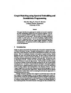
To illustrate the effectiveness of the adjacency spectral embedding, we simulate random undirected graphs generated from the following stochastic blockmodel: ! 0.42 0.42 and ρ = (.6, .4)T (23) P= 0.42 0.5 For each n ∈ {500, 600, . . . , 2000}, we simulated 100 monte carlo replicates from this model conditioned on the fact that |{u ∈ [n] : τ (u) = i}| = ρi n for each i ∈ {1, 2}. In this model we assume that d = 2 and K = 2 are known. We evaluated four different embedding procedures and for each embedding we used K-means clustering, which attempts to iteratively find the solution to Eqn. 4, to generate the node assignment function τˆ. The four embedding procedure are the scaled and unscaled adjacency spectral embedding as well as the scaled and unscaled Laplacian spectral embedding. The Laplacian spectral embedding uses the same spectral decomposition but works with the normalized Laplacian (as defined in Rohe et al. (2011)) rather then the adjacency matrix. The normalized Laplacian is given by L = D−1/2 AD−1/2 where D ∈ Rn×n is diagonal with Dvv = deg(v), the degree of node v. We evaluated the performance of the node assignments by computing the percentage of mis-assigned nodes, minπ∈S2 |{u ∈ [n] : τ (u) 6= π(ˆ τ (u))}|/n, as in Eqn. 6. Figure 1 demonstrates that performance of K-means on all four embeddings improves with increasing number of nodes. It also demonstrates (via a paired Wilcoxon test) that for these model parameters the adjacency embedding is superior to the Laplacian embeddings for large n. In fact, for n ≥ 1400 we observed that for each simulated graph the scaled adjacency embedding always performed better than both Laplacian embeddings. We note that these
12
0.50
Adjacency (Scaled) Adjacency (Unscaled) Laplacian (Scaled) Laplacian (Unscaled)
0.45 0.40 Percent Error
0.35 0.30 0.25 0.20 0.15 0.10 0.05 400
600
800
1000 1200 1400 n - Number of vertices
1600
1800
2000
Figure 1: Mean error for 100 monte carlo replicates using K-means on four different embedding procedures. model parameters were specifically constructed to demonstrate a case where the adjacency embedding is superior to the Laplacian embedding. Figure 2 shows an example of the scaled adjacency (left) and scaled Laplacian (right) spectral embeddings. The graph has 2000 nodes and the points are colored according to their block membership. The dashed line shows the discriminant boundary given by the K-means algorithm with K = 2.
6.2
Wikipedia Graph
For this data, each node in the graph corresponds to a Wikipedia page and the edges correspond to the presence of a hyperlink between two pages (in either direction). We consider this as an undirected graph. Every article within two hyperlinks of the article “Algebraic Geometry” was included as a node in the graph. This resulted in n = 1382 nodes. Additionally, each document, and hence each node, was manually labeled as one of the following: Category, Person, Location, Date and Math. To illustrate the utility of this algorithm we embedded this graph using the scaled adjacency and Laplacian procedures. Figure 3 shows the two embeddings for d = 2. The points are colored according to their manually assigned labels. First we note that on the whole the two embeddings look moderately different. In fact, for the adjacency embedding one can see that the orange points are well separated from the remaining data. On the other hand, with the Laplacian embedding we can see that the red points are somewhat separated from the remaining data. The dashed lines show the result boundary as determined by K-means with K = 2. To evaluate the performance we considered the 5 different tasks of identifying one block and grouping the remaining blocks together. For each of the 5 blocks,
13
0.6
0.020 0.015
0.4
0.010 0.2
0.005
0.0
0.000 −0.005
−0.2
−0.010 −0.4 −0.6
−0.015 −1.0
−0.8
−0.6
−0.4
−0.2
−0.020
−0.035 −0.030 −0.025 −0.020 −0.015 −0.010
Figure 2: Scatter plots of the scaled adjacency (left) and Laplacian (right) embeddings of a 2000 node graph. we compared each of the one-vs-all block labels to the estimated labels from K-means, with K = 2, on the two embeddings. Table 1 shows the number of incorrectly assigned nodes, as in Eqn. 6, as well as the adjusted Rand index (Hubert and Arabie, 1985). The adjusted Rand index (ARI) has the property that the optimal value is 1 and a value of zero indicates the expected value if the labels were assigned randomly. We can see from this table that K-means on the adjacency embedding identifies the separation of the Date block from the other four while on the Laplacian embedding K-means identifies the separation of the Math block from the other four. This indicates that for this data set (and indeed more generally) the choice of embedding procedure will depend greatly on the desired exploitation task. We note that for both embeddings, the clusters generated using K-means, with K = 5, poorly reflect the manually assigned block memberships. We have not investigated beyond the illustrative 2-dimensional embeddings. Category (119) Error ARI
Person (372) Error ARI
Location (270) Error ARI
Date (191) Error ARI
Math (430) Error ARI
A
242
-0.08
495
-0.07
341
0.01
130
0.47
543
0.06
L
299
-0.02
495
-0.02
476
-0.1
401
-0.10
350
0.19
Table 1: One versus all comparison of each block against the estimated K-means block assignments with K = 2.
14
1.5
Adjacency
Laplacian
0.10 0.05
1.0 0.00 0.5
−0.05 −0.10
0.0
−0.15
−0.5
−0.20
−1.0 −1.6 −1.4 −1.2 −1.0 −0.8 −0.6 −0.4 −0.2
0.0
0.2
−0.25 −0.02
0.00
0.02
0.04
0.06
0.08
0.10
0.12
Figure 3: Scatter plots for the Wikipedia graph. The left pane show the scaled adjacency embedding and the right pane show the scaled Laplacian embedding. Each point is colored according to the manually assigned labels. The dashed line represents the discriminant boundary determined by K-means with K = 2.
7
Discussion
Our simulations demonstrate that for a particular example of the stochastic blockmodel, the proportion of mis-assigned nodes will rapidly become small. Though our bound shows that the number of mis-assigned nodes will not grow faster than O(log n), in some instances this bound may be very loose. We also demonstrate that using the adjacency embedding over the Laplacian embedding can provide performance improvements in some settings. It is also clear from Figure 2 that the use of other unsupervised clustering techniques, such as Gaussian mixture modeling, will likely lead to further performance improvements. On the Wikipedia graph, the two-dimensional embedding demonstrates that the adjacency embedding procedure provides an alternative to the Laplacian embedding and the two may have fundamentally different properties. Both the Date block and the Math block have some differentiating structure in the graph but these structures are illuminated more in one embedding then the other. This analysis suggests that further investigations into comparisons between the adjacency embedding and the Laplacian embeddings will be fruitful. Our empirical analysis indicates that the adjacency spectral embeddings and the Laplacian spectral embeddings are strongly related while the two embeddings may emphasize different aspects of the particular graph. Rohe et al. (2011) used similar techniques to show consistency of block assignment on the Laplacian embedding and achieved the same asymptotic rates of misclassification. e then this embedding Indeed, if one considers the embedding given by D−1/2 X, will be very close to the scaled Laplacian embedding and may provide a link between the two procedures. Note that consistent block assignments are possible using either the singular
15
vectors or the scaled version of the singular vectors. The singular vectors themselves are essentially a whitened version of scaled singular vectors. Since the singular vectors are orthogonal, the estimated covariance of rows of the scaled vectors is proportional to the diagonal matrix given by the singular values of A. This suggests that clustering using a criterion invariant to coordinate-scalings and rotations will likely have similar asymptotic properties. Critical to the proof is the bound provided by Proposition 2. Since this bound does not depend on the method for generating Q, it suggests that extensions to this theorem are possible. One such extension is to take the number of blocks K = Kn to go slowly to infinity. For Kn growing, the parameters α, β, and γ are no longer constant in n, so we must impose conditions on these parameters. If we take d fixed and assume these parameters go to 0 slowly, it is possible to allow Kn = n� for � sufficiently small. Under these conditions, it can be shown that the number of incorrect block assignments is o(nγ), which is negligible to block sizes. Our proof technique breaks down for Kn = Ω(n1/4 ) as Proposition 2 no longer implies a gap in the singular values of A. In order to avoid the model selection quagmire, we assumed in Theorem 1 that the number of blocks K and the latent feature dimension d are known. However, the proof of this theorem suggests that both K and and d can be estimated consistently. Corollary 5, shows that all but d of the singular values of A are less than 31/4 n3/4 log1/4 n for n large enough. As discussed earlier, this shows that dˆ = max{i : σi (A) > 31/4 n3/4 log1/4 n} will be a consistent estimator for d. Though this estimator is consistent, the required number of nodes for it to become accurate will depend highly on the sparsity of the graph, which controls the magnitude of the largest singular values of A. Furthermore, our bounds suggest that the number of nodes required for this estimate to be accurate will increase exponentially as the expected graph density decreases. Estimating K is more complicated, and we do not present a formal method to do so. We do note that the proof shows that most of the embedded vectors are concentrated around K separated points. An appropriate covering of the points by slowly vanishing balls would allow for a consistent estimate of K. More work is needed to provide model selection criteria which are practical to the practitioner. Note that some practitioners may have estimates or bounds for the parameters P and ρ, derived from some prior study. In this case, provided bounds on α, β, and γ can be determined, the proof can be used to derive high probability bounds on the number of nodes that have been assigned to the incorrect block. This may also enable the practitioner to choose n to optimize some misassignment and cost criteria. The proofs above would remain valid if the diagonals of the adjacency matrix are modified provided that each modification is bounded. In fact, modifying the diagonals may improve the embedding to give lower numbers of misassignments. Marchette et al. (2011) suggests replacing the diagonal element Auu with deg(u)/(n − 1) for each node u ∈ [n]. Scheinerman and Tucker (2010) provided an iterative algorithm to impute the diagonal. An optimal choice the diagonal is not known for general stochastic blockmodels. 16
Another practical concern is the possibility of missing data in the observed graph. One example may be that each edge in the true graph is only observed with probability p in the observed graph. Our theory will be unaffected by this type of error since the observed graph is also distributed according to a stochastic blockmodel with edge probabilities P0 = pP. As a result, asymptotic consistency remains valid. We may also allow p to decrease slowly with n and still achieve asymptotically negligible misassignments. However, typically the finite sample performance will if p is small. Overall, the theory and results presented suggest that this embedding procedure is worthy of further investigation. The problems estimating K and d, choosing between scaled and unscaled embedding and between the adjacency and the Laplacian will all be considered in future work. This work is also being generalized to more general latent position models. Finally, under the stochastic blockmodel, our method will be less computationally demanding than ones which depend on maximizing likelihood or modularity criterion. Fast methods to compute singular value decompositions are possible, especially for sparse matrices. There are a plethora of methods for efficiently clustering points in Euclidean space. Overall, this embedding method may be valuable to the practitioner to provide a rapid method to identify blocks in networks.
A
Proofs of Technical Lemmas
In this appendix, we prove the technical results stated in Section 3.2. Lemma 4. It almost always holds that αγn ≤ σd (XYT ) and it always holds that σd+1 (XYT ) = 0 and σ1 (XYT ) ≤ n. Proof. Since XYT ∈ [0, 1]n×n , the nonnegative matrix XYT (XYT )T has entries bounded by n. The row sums are bounded by n2 giving that σ12 (XYT ) = λ1 (XYT (XYT )T ) ≤ n2 . Since X and Y are at most rank d, we have σd+1 (XY) = 0. The nonzero eigenvalues of XYT (XYT )T = XYT YT X are the same as the nonzero eigenvalues of YT YXT X. It almost always holds that ni ≥ γn for all i so that K K X X XT X = ni νi νiT = γnν T ν + (ni − γn)νi νiT (24) i=1
i=1
is the sum of two positive semidefinite matrices, the first of which has eigenvalues all greater then αγn. This gives λd (XT X) ≥ αγn and similarly λd (YT Y) ≥ αγn. This gives that YT YXT X is the product of positive definite matrices. We then use a bound on the smallest eigenvalues of the product of two positive semi-definite matrices, so that λd (YT YXT X) ≥ λd (YT Y)λd (XT X) ≥ (αγn)2 (Zhang and Zhang, 2006, Corollary 11). This establishes σd2 (XYT ) ≥ (αγn)2 .
17
Corollary 5. It almost always holds that αγn ≤ σd (A) and σd+1 (A) ≤ 31/4 n3/4 log1/4 n and it always holds that σ1 (A) ≤ n. Proof. First, by the same arguments as Lemma 4 we have σ1 (A) ≤ n. By Weyl’s inequality (Horn and Johnson, 1985, §6.3), we have that |σi2 (A) − σi2 (XYT )| = |λi (AAT ) − λi (XYT (XYT )T )| ≤ kAAT − XYT (XYT )T kF .
(25)
Together with Corollary 3 this shows that σd+1 (A) ≤ 31/4 n3/4 log1/4 n almost always. Since γ < ρi for each i, Lemma 4 can be strengthened to show that there exists � > 0, not dependent on n, such that (αγ + �)n < σd (XYT ). Thus, (αγ + �)2 n2 < σd2 (XYT ) so that (αγ)2 n2 ≤ σd2 (A) since √ 3/2we √ have that 2 2 3n log n < � n for n large enough. The singular value decomposition of XYT is given b UΣVT . The next result provides bounds for the gaps between the at most K distinct rows of U and V. Recall that for a matrix M, row u is given MuT for all u. Lemma 8. It almost always holds that, for all u, v such that Xu 6= Xv , kUu − √ √ Uv k ≥ β αγn−1/2 . Similarly, for all Yu 6= Yv , kVu − Vv k ≥ β αγn−1/2 . As a √ result, kWu − Wv k ≥ β αγn−1/2 for all u, v such that τ (u) 6= τ (v).
Proof. Let YT Y = ED2 ET for E ∈ Rd×d orthogonal, D ∈ Rd×d diagonal. Define G = XE, G0 = GD, and U0 = UΣ. Let u, v be such that Xu 6= Xv . √ From Lemma 4 and its proof, diagonals of D are almost always at least αγn and the diagonals of Σ are at most n. Now, G0 G0T = GD2 GT = XED2 ET XT = XYT YXT = UΣVT VΣUT = UΣ2 UT = U0 U0T .
(26)
Let e ∈ Rn denote the vector with all zeros except 1 in the uth coordinate and −1 in the v th coordinate. By the above we have kG0u − G0v k2 = eT G0 G0T e = eT U0 U0T e = kUu0 − Uv0 k2 . Therefore we obtain that β ≤ kXu − Xv k = kGu − 1 1 1 Gv k ≤ √αγn kG0u − G0v k = √αγn kUu0 − Uv0 k ≤ √αγn nkUu − Uv k, as desired. A symmetric argument holds for kVu − Vv k. For kWu − Wv k note that if τ (u) 6= τ (v) then either Uu 6= Uv or Vu 6= Vv . Lemma 7. It almost always holds that there exists an orthogonal matrix R ∈ √ √6 q log n 2d×2d f ≤ 2 2 2 R such that kWR − Wk . α γ
( 12 α2 γ 2 n2 , ∞).
n
Proof. Let S = By Lemma 4 and Corollary 5, it almost always holds that exactly d eigenvalues of AAT and XYT (XYT )T are in S. Additionally, Lemma 4 shows that the gap δ > α2 γ 2 n2 . Together with Corollary 3, we have that √ √ √ kAAT − XYT (XYT )T kF √ 3n3/2 log n 2 ≤ 2 . (27) δ α 2 γ 2 n2 18
e F ≤ This shows there exists an R1 ∈ Rd×d such that kUR1 − Uk
√ q log n 6 α2 γ 2 n . T T T
Now note that all of the above could be repeated for AT A and (XY ) XY , √ q e F ≤ 2 62 log n . Taking R as the direct to find R2 ∈ Rd×d such that kVR2 − Vk α γ
n
sum of R1 and R2 gives the result.
B
Davis-Kahan Theorem
We now state and provide a brief discussion of the Davis-Kahan theorem (Davis and Kahan, 1970; Rohe et al., 2011). First, we consider some general results from the theory of Grassmann spaces (Qi et al., 2005). Let Gd,n denote the set of d-dimensional subspaces of Rn . Two important metrics on Gd,n are the gap metric dg and the Hausdorff metric dh which are defined as follows. For all W, W 0 ∈ Gd,n , v u d uX 0 sin2 θi (W, W 0 ) (28) dg (W, W ) = t i=1
v u d � �2 uX θi (W, W 0 ) 0 t dh (W, W ) = 2 sin 2 i=1
(29)
where θ1 (W, W 0 ), θ2 (W, W 0 ), . . . θd (W, W 0 ) denote the √principal angles between W and W 0 . By simple trigonometry dh (W, W 0 ) ≤ 2 · dg (W, W 0 ). Suppose W, W0 ∈ Rn,d have columns which are orthonormal bases for W and W 0 , respectively. It is well known that dh (W, W 0 ) = minR kWR − W0 kF where the minimum is over all orthogonal matrices R ∈ Rd×d . The next theorem states the original form of the theorem from Davis and Kahan (1970) followed by the version proved in Rohe et al. (2011). Theorem 6 (Davis and Kahan). Let H, H0 ∈ Rn×n be symmetric, suppose S ⊂ R is an interval, and suppose for some positive integer d that W ∈ Gd,n is the sum of the eigenspaces of H associated with the eigenvalues of H in S, and that W 0 ∈ Gd,n is the sum of the eigenspaces of H0 associated with the eigenvalues of H0 in S. If δ is the minimum distance between any eigenvalue of H in S and any eigenvalue of H not in S then δ · dg (W, W 0 ) ≤ kH − H0 kF . Furthermore, suppose W, W0 ∈ Rn×d are such that the columns of W form an orthonormal basis for W and that the columns W0 form an orthonormal basis for W 0 . Then there exists an orthogonal matrix R ∈ Rd×d such that √ 2 0 kWR − W kF ≤ δ kH − H0 kF . From the preceding analysis we see that the version from Rohe et al. (2011) follows from the original theorem; indeed, we have for some orthogonal R ∈ √ √ 2 d×d 0 0 0 R that kWR − R kF = dh (W, W ) ≤ 2dg (W, W ) ≤ δ kH − H0 kF .
19
References E. M. Airoldi, D. M. Blei, S. E. Fienberg, and E. P. Xing. Mixed membership stochastic blockmodels. The Journal of Machine Learning Research, 9:1981– 2014, 2008. 2 P. J. Bickel and A. Chen. A nonparametric view of network models and Newman-Girvan and other modularities. Proceedings of the National Academy of Sciences of the United States of America, 106:21068–21073, 2009. 3 D. S. Choi, P. J. Wolfe, and E. M. Airoldi. Stochastic blockmodels with growing number of classes. Biometrika, In press. 3 A. Condon and R. M. Karp. Algorithms for graph partitioning on the planted partition model. Random Structures and Algorithms, 18:116–140, 2001. 3 C. Davis and W. Kahan. The rotation of eigenvectors by a pertubation. III. Siam Journal on Numerical Analysis, 7:1–46, 1970. 8, 9, 19 C. Eckart and G. Young. The approximation of one matrix by another of lower rank. Psychometika, 1:211–218, 1936. 5 P. Fjallstrom. Algorithms for graph partitioning: A survey. Computer and Information Science, 3(10), 1998. 2 S. Fortunato. Community detection in graphs. Physics Reports, 486:75–174, 2010. 2 A. Goldenberg, A. X. Zheng, S. E. Fienberg, and E. M. Airoldi. A survey of statistical network models. Foundations and Trends in Machine Learning, 2, 2010. 2 M. S. Handcock, A. E. Raftery, and J. M. Tantrum. Model-based clustering for social networks. Journal of the Royal Statistical Society: Series A (Statistics in Society), 170:301–354, 2007. 2 P. Hoff, A. E. Raftery, and M. S. Handcock. Latent space approaches to social network analysis. Journal of the American Statistical Association, 97:1090– 1098, 2002. 2 P. W. Holland, K. Laskey, and S. Leinhardt. Stochastic blockmodels: First steps. Social Networks, 5:109–137, 1983. 2, 4 R. Horn and C. Johnson. Matrix Analysis. Cambridge University Press, 1985. 18 L. Hubert and P. Arabie. Comparing partitions. Journal of Classification, 2: 193–218, 1985. 14 D. J. Marchette, C. E. Priebe, and G. Coppersmith. Vertex nomination via attributed random dot product graphs. In Proceedings of the 57th ISI World Statistics Congress, 2011. 6, 16 20
F. McSherry. Spectral partitioning of random graphs. In Proceedings of the 42nd IEEE symposium on Foundations of Computer Science, pages 529–537. IEEE Computer Society, 2001. 3 M. Newman and M. Girvan. Finding and evaluating community structure in networks. Physical Review, 69:1–15, 2004. 3 K. Nowicki and T. A. B. Snijders. Estimation and Prediction for Stochastic Blockstructures. Journal of the American Statistical Association, 96:1077– 1087, 2001. 2 L. Qi, Y. Zhang, and C.-K Li. Unitarily Invariant Metrics on the Grassmann Space. SIAM Journal on Matrix Analysis and Applications, 27:507–531, 2005. 19 K. Rohe, S. Chatterjee, and B. Yu. Spectral clustering and the high-dimensional stochastic blockmodel. Annals of Statistics, 39:1878–1915, 2011. 3, 8, 9, 12, 15, 19 E. Scheinerman and K. Tucker. Modeling graphs using dot product representations. Computational Statistics, 25:1–16, 2010. 16 T. Snijders and K. Nowicki. Estimation and prediction for stocchastic block models for graphs with latent block structure. Journal of Classification, 14: 75–100, 1997. 2, 3 Y. J. Wang and G. Y. Wong. Stochastic Blockmodels for Directed Graphs. Journal of the American Statistical Association, 82:8–19, 1987. 2, 4 S. Young and E. Scheinerman. Random dot product models for social networks. In Proceedings of the 5th international conference on algorithms and models for the web-graph, pages 138–149, 2007. 2 F. Zhang and Q. Zhang. Eigenvalue inequalities for matrix product. Automatic Control, IEEE Transactions on, 51:1506–1509, 2006. 17
21